
When we write complex behavioral models it is useful to divide the code into sections, each dealing with a relatively self-contained part of the behavior. VHDL provides a subprogram facility to let us do this. In this chapter, we look at the two kinds of subprograms: procedures and functions. The difference between the two is that a procedure encapsulates a collection of sequential statements that are executed for their effect, whereas a function encapsulates a collection of statements that compute a result. Thus a procedure is a generalization of a statement, whereas a function is a generalization of an expression.
We start our discussion of subprograms with procedures. There are two aspects to using procedures in a model: first the procedure is declared, then elsewhere the procedure is called. The syntax rule for a procedure declaration is
   subprogram_body ⇐
      procedure identifier [(parameter_interface_list)]is
           {subprogram_declarative_part}
      begin
           {sequential_statement}
      end [ procedure ] [ identifier ] ;
For now we will just look at procedures without the parameter list part; we will come back to parameters in the next section.
The identifier in a procedure declaration names the procedure. The name may be repeated at the end of the procedure declaration. The sequential statements in the body of a procedure implement the algorithm that the procedure is to perform and can include any of the sequential statements that we have seen in previous chapters. A procedure can declare items in its declarative part for use in the statements in the procedure body. The declarations can include types, subtypes, constants, variables and nested subprogram declarations. The items declared are not accessible outside of the procedure; we say they are local to the procedure.
Example 6.1. Averaging an array of data samples
The following procedure calculates the average of a collection of data values stored in an array called samples and assigns the result to a variable called average. This procedure has a local variable total for accumulating the sum of array elements. Unlike variables in processes, procedure local variables are created anew and initialized each time the procedure is called.
   procedure average_samples is
     variable total : real := 0.0;
   begin
     assert samples'length > 0 severity failure;
     for index in samples'range loop
      total := total + samples(index);
     end loop;
     average := total / real(samples'length);
   end procedure average_samples;
The actions of a procedure are invoked by a procedure call statement, which is yet another VHDL sequential statement. A procedure with no parameters is called simply by writing its name, as shown by the syntax rule
procedure_call_statement ⇐ [ label : ] procedure_name ;The optional label allows us to identify the procedure call statement. We will discuss labeled statements in Chapter 20. As an example, we might include the following statement in a process:
average_samples;
The effect of this statement is to invoke the procedure average_samples. This involves creating and initializing a new instance of the local variable total, then executing the statements in the body of the procedure. When the last statement in the procedure is completed, we say the procedure returns; that is, the thread of control of statement execution returns to the process from which the procedure was called, and the next statement in the process after the call is executed.
We can write a procedure declaration in the declarative part of an architecture body or a process. We can also declare procedures within other procedures, but we will leave that until a later section. If a procedure is included in an architecture body’s declarative part, it can be called from within any of the processes in the architecture body. On the other hand, declaring a procedure within a process hides it away from use by other processes.
Example 6.2. A procedure to implement behavior within a process
The outline below illustrates a procedure defined within a process. The procedure do_arith_op encapsulates an algorithm for arithmetic operations on two values, producing a result and a flag indicating whether the result is zero. It has a variable result, which it uses within the sequential statements that implement the algorithm. The statements also use the signals and other objects declared in the architecture body. The process alu invokes do_arith_op with a procedure call statement. The advantage of separating the statements for arithmetic operations into a procedure in this example is that it simplifies the body of the alu process.
   architecture rtl of control_processor is

     type func_code is (add, subtract);

     signal op1, op2, dest : integer;
     signal Z_flag : boolean;
     signal func : func_code;
     ...
   begin

     alu : process is
      procedure do_arith_op is
        variable result : integer;
      begin
        case func is
          when add =>
            result := op1 + op2;
          when subtract =>
            result := op1 - op2;
        end case;
        dest  <=  result after Tpd;
        Z_flag  <=  result = 0 after Tpd;
      end procedure do_arith_op;
     begin
      ...
      do_arith_op;
      ...
     end process alu;
     ...
   end architecture rtl;
Another important use of procedures arises when some action needs to be performed several times at different places in a model. Instead of writing several copies of the statements to perform the action, the statements can be encapsulated in a procedure, which is then called from each place.
Example 6.3. A memory read procedure invoked from several places in a model
The process outlined below is taken from a behavioral model of a CPU. The process fetches instructions from memory and interprets them. Since the actions required to fetch an instruction and to fetch a data word are identical, the process encapsulates them in a procedure, read_memory. The procedure copies the address from the memory address register to the address bus, sets the read signal to ‘1’, then activates the request signal. When the memory responds, the procedure copies the data from the data bus signal to the memory data register and acknowledges to the memory by setting the request signal back to ‘0’. When the memory has completed its operation, the procedure returns.
   instruction_interpreter : process is

    variable mem_address_reg, mem_data_reg,
             prog_counter, instr_reg, accumulator, index_reg : word;
    ...
    procedure read_memory is
    begin
      address_bus <= mem_address_reg;
      mem_read <= '1';
      mem_request <= '1';
      wait until mem_ready;
      mem_data_reg := data_bus_in;
      mem_request <= '0';
      wait until not mem_ready;
    end procedure read_memory;
   begin
    ...  -- initialization
    loop
      -- fetch next instruction
      mem_address_reg := prog_counter;
      read_memory;      -- call procedure
      instr_reg := mem_data_reg;
      ...
      case opcode is
        ...
        when load_mem =>
          mem_address_reg := index_reg + displacement;
          read_memory;  -- call procedure
          accumulator := mem_data_reg;
        ...
      end case;

    end loop;
   end process instruction_interpreter;
The procedure is called in two places within the process. First, it is called to fetch an instruction. The process copies the program counter into the memory address register and calls the procedure. When the procedure returns, the process copies the data from the memory data register, placed there by the procedure, to the instruction register. The second call to the procedure takes place when a “load memory” instruction is executed. The process sets the memory address register using the values of the index register and some displacement, then calls the memory read procedure to perform the read operation. When it returns, the process copies the data to the accumulator.
Since a procedure call is a form of sequential statement and a procedure body implements an algorithm using sequential statements, there is no reason why one procedure cannot call another procedure. In this case, control is passed from the calling procedure to the called procedure to execute its statements. When the called procedure returns, the calling procedure carries on executing statements until it returns to its caller.
Example 6.4. Nested procedure calls in a control sequencer
The process outlined below is a control sequencer for a register-transfer-level model of a CPU. It sequences the activation of control signals with a two-phase clock on signals phase1 and phase2. The process contains two procedures, control_write_back and control_arith_op, that encapsulate parts of the control algorithm. The process calls control_arith_op when an arithmetic operation must be performed. This procedure sequences the control signals for the source and destination operand registers in the data path. It then calls control_write_back, which sequences the control signals for the register file in the data path, to write the value from the destination register. When this procedure is completed, it returns to the first procedure, which then returns to the process.
   control_sequencer : process is

    procedure control_write_back is
    begin
      wait until phase1;
      reg_file_write_en <= '1';
      wait until not phase2;
      reg_file_write_en <= '0';
    end procedure control_write_back;
    procedure control_arith_op is
    begin
      wait until phase1;
      A_reg_out_en <= '1';
      B_reg_out_en <= '1';

      wait until not phase1;
      A_reg_out_en <= '0';
      B_reg_out_en <= '0';
      wait until phase2;
      C_reg_load_en <= '1';
      wait until not phase2;
      C_reg_load_en <= '0';
      control_write_back;  -- call procedure
    end procedure control_arith_op;
    ...
   begin
    ...
    control_arith_op;  -- call procedure
    ...
   end process control_sequencer;
VHDL-87
The keyword procedure may not be included at the end of a procedure declaration in VHDL-87. Procedure call statements may not be labeled in VHDL-87.
In all of the examples above, the procedures completed execution of the statements in their bodies before returning. Sometimes it is useful to be able to return from the middle of a procedure, for example, as a way of handling an exceptional condition. We can do this using a return statement, described by the simplified syntax rule
return_statement ⇐ [label :] return ;
The optional label allows us to identify the return statement. We will discuss labeled statements in Chapter 20. The effect of the return statement, when executed in a procedure, is that the procedure is immediately terminated and control is transferred back to the caller.
Example 6.5. A revised memory read procedure
The following is a revised version of the instruction interpreter process from Example 6.3. The procedure to read from memory is revised to check for the reset signal becoming active during a read operation. If it does, the procedure returns immediately, aborting the operation in progress. The process then exits the fetch/execute loop and starts the process body again, reinitializing its state and output signals.
   instruction_interpreter : process is
    ...

    procedure read_memory is
    begin
      address_bus <= mem_address_reg;
      mem_read <= '1';
      mem_request <= '1';
      wait until mem_ready or reset;
      if reset then
        return;
      end if;
      mem_data_reg := data_bus_in;
      mem_request <= '0';
      wait until not mem_ready;
    end procedure read_memory;
   begin
    ...    -- initialization
    loop
      ...
      read_memory;
      exit when reset;
        ...
    end loop;
   end process instruction_interpreter;
Now that we have looked at the basics of procedures, we will discuss procedures that include parameters. A parameterized procedure is much more general in that it can perform its algorithm using different data objects or values each time it is called. The idea is that the caller passes parameters to the procedure as part of the procedure call, and the procedure then executes its statements using the parameters.
When we write a parameterized procedure, we include information in the parameter interface list (or parameter list, for short) about the parameters to be passed to the procedure. The syntax rule for a procedure declaration on page 207 shows where the parameter list fits in. Following is the syntax rule for a parameter list:
   interface_list ⇐
       {[constant |variable | signal
          identifier {, ...}: [ mode] subtype_indication
                                           [:= static_expression]} {; ...}
   mode ⇐ in | out| inout
As we can see, it is similar to the port interface list used in declaring entities. This similarity is not coincidental, since they both specify information about objects upon which the user and the implementation must agree. In the case of a procedure, the user is the caller of the procedure, and the implementation is the body of statements within the procedure. The objects defined in the parameter list are called the formal parameters of the procedure. We can think of them as placeholders that stand for the actual parameters, which are to be supplied by the caller when it calls the procedure. Since the syntax rule for a parameter list is quite complex, let us start with some simple examples and work up from them.
Example 6.6. Using a parameter to select an arithmetic operation to perform
Let’s rewrite the procedure do_arith_op from Example 6.2 so that the function code is passed as a parameter. The new version is
   procedure do_arith_op ( op : in func_code ) is
    variable result : integer;
   begin
    case op is
      when add =>
        result := op1 + op2;
      when subtract =>
        result := op1 - op2;
    end case;
    dest  <=  result after Tpd;
    Z_flag  <=  result = 0 after Tpd;
   end procedure do_arith_op;
In the parameter interface list we have identified one formal parameter named op. This name is used in the statements in the procedure to refer to the value that will be passed as an actual parameter when the procedure is called. The mode of the formal parameter is in, indicating that it is used to pass information into the procedure from the caller. This means that the statements in the procedure can use the value but cannot modify it. In the parameter list we have specified the type of the parameter as func_code. This indicates that the operations performed on the value in the statements must be appropriate for a value of this type, and that the caller may only pass a value of this type as an actual parameter.
Now that we have parameterized the procedure, we can call it from different places passing different function codes each time. For example, a call at one place might be
do_arith_op ( add );
The procedure call simply includes the actual parameter value in parentheses. In this case we pass the literal value add as the actual parameter. At another place in the model we might pass the value of the signal func shown in the model in Example 6.2:
do_arith_op ( func );
In this example, we have specified the mode of the formal parameter as in. Note that the syntax rule for a parameter list indicates that the mode is an optional part. If we leave it out, mode in is assumed, so we could have written the procedure as
procedure do_arith_op ( op : func_code ) is ...
While this is equally correct, it’s not a bad idea to include the mode specification for in parameters, to make our intention explicitly clear.
The syntax rule for a parameter list also shows us that we can specify the class of a formal parameter, namely, whether it is a constant, a variable or a signal within the procedure. If the mode of the parameter is in, the class is assumed to be constant, since a constant is an object that cannot be updated by assignment. It is just a quirk of VHDL that we can specify both constant and in, even though to do so is redundant. Usually we simply leave out the keyword constant, relying on the mode to make our intentions clear. (The exceptions are parameters of access types, discussed in Chapter 15, and file types, discussed in Chapter 16.) For an in-mode constant-class parameter, we write an expression as the actual parameter. The value of this expression must be of the type specified in the parameter list. The value is passed to the procedure for use in the statements in its body.
Let us now turn to formal parameters of mode out. Such a parameter lets us transfer information out from the procedure back to the caller. Here is an example, before we delve into the details.
Example 6.7. A procedure for addition with overflow output
The procedure below performs addition of two unsigned numbers represented as bit vectors of type word32, which we assume is defined elsewhere. The procedure has two in-mode parameters a and b, allowing the caller to pass two bit-vector values. The procedure uses these values to calculate the sum and overflow flag. Within the procedure, the two out-mode parameters, sum and overflow, appear as variables. The procedure performs variable assignments to update their values, thus transferring information back to the caller.
   procedure addu (a, b : in word32;
                   sum : out word32;
                   overflow : out bit ) is
    variable carry : bit := '0';
   begin
    for index in sum'reverse_range loop
      sum(index) := a(index) xor b(index) xor carry;
      carry := ( a(index) and b(index) )
               or ( carry and ( a(index) xor b(index) ) );
    end loop;
    overflow := carry;
   end procedure addu;
A call to this procedure may appear as follows:
   variable PC, next_PC : word32;
   variable overflow_flag : bit;
   ...
   addu ( PC, X"0000_0004", next_PC, overflow_flag);
In this procedure call statement, the first two actual parameters are expressions whose values are passed in through the formal parameters a and b. The third and fourth actual parameters are the names of variables. When the procedure returns, the values assigned by the procedure to the formal parameters sum and overflow are used to update the variables next_PC and overflow_flag.
In the above example, the out-mode parameters are of the class variable. Since this class is assumed for out parameters, we usually leave out the class specification variable, although it may be included if we wish to state the class explicitly. We will come back to signal-class parameters in a moment. The mode out indicates that the procedure may update the formal parameters by variable assignment to transfer information back to the caller. The procedure may also read the values of the parameters, just as it can with in-mode parameters. The difference is that an out-mode parameter is not initialized with the value of the actual parameter. Instead, it is initalized in the same way as a locally declared variable, with the default initial value for the type of the parameter. When the procedure reads the parameter, it reads the parameter’s current value, yielding the value most recently assigned within the procedure, or the initial value if no assignments have been made. For an out mode, variable-class parameter, the caller must supply a variable as an actual parameter. Both the actual parameter and the value returned must be of the type specified in the parameter list. When the procedure returns, the value of the formal parameter is copied back to the actual parameter variable.
The third mode we can specify for formal parameters is inout, which is a combination of in and out modes. It is used for objects that are to be both read and updated by a procedure. As with out parameters, they are assumed to be of class variable if the class is not explicitly stated. For inout-mode variable parameters, the caller supplies a variable as an actual parameter. The value of this variable is used to initialize the formal parameter, which may then be used in the statements of the procedure. The procedure may also perform variable assignments to update the formal parameter. When the procedure returns, the value of the formal parameter is copied back to the actual parameter variable, transferring information back to the caller.
Example 6.8. A procedure to negate a binary-coded number
The following procedure negates a number represented as a bit vector, using the “complement and add one” method:
   procedure negate ( a : inout word32 ) is
     variable carry_in : bit := '1';
     variable carry_out : bit;

   begin
     a := not a;
     for index in a'reverse_range loop
      carry_out :=  a(index) and carry_in;
      a(index) := a(index) xor carry_in;
      carry_in := carry_out;
     end loop;
   end procedure negate;
Since a is an inout-mode parameter, we can refer to its value in expressions in the procedure body. (This differs from the parameter result in the addu procedure of the previous example.) We might include the following call to this procedure in a model:
   variable op1 : word32;
   ...
   negate ( op1 );
This uses the value of op1 to initialize the formal parameter a. The procedure body is then executed, updating a, and when it returns, the final value of a is copied back into op1.
VHDL-87, -93, and -2002
These versions of VHDL do not allow an out-mode parameter to be read. Instead, if the value must be read within the procedure, the procedure must declare and read a local variable. The final value of the local variable can then be assigned to the out-mode parameter immediately before the procedure returns.
The third class of object that we can specify for formal parameters is signal, which indicates that the algorithm performed by the procedure involves a signal passed by the caller. A signal parameter can be of any of the modes in, out or inout. The way that signal parameters work is somewhat different from constant and variable parameters, so it is worth spending a bit of time understanding them.
When a caller passes a signal as a parameter of mode in, instead of passing the value of the signal, it passes the signal object itself. Any reference to the formal parameter within the procedure is exactly like a reference to the actual signal itself. The statements within the procedure can read the signal value, include it in sensitivity lists in wait statements, and query its attributes. A consequence of passing a reference to the signal is that if the procedure executes a wait statement, the signal value may be different after the wait statement completes and the procedure resumes. This behavior differs from that of constant parameters of mode in, which have the same value for the whole of the procedure.
Example 6.9. A procedure to receive network packets
Suppose we wish to model the receiver part of a network interface. It receives fixed-length packets of data on the signal rx_data. The data is synchronized with changes, from ‘0’ to ‘1’, of the clock signal rx_clock. An outline of part of the model is
   architecture behavioral of receiver is
    ...    -- type declarations, etc
    signal recovered_data : bit;
    signal recovered_clock : bit;
    ...
    procedure receive_packet ( signal rx_data : in bit;
                               signal rx_clock : in bit;
                               data_buffer : out packet_array ) is
    begin
      for index in packet_index_range loop
        wait until rx_clock;
        data_buffer(index) := rx_data;
      end loop;
    end procedure receive_packet;
   begin
    packet_assembler : process is
      variable packet : packet_array;
    begin
      ...
      receive_packet ( recovered_data, recovered_clock, packet );
      ...
    end process packet_assembler;
    ...
   end architecture behavioral;
The receive_packet procedure has signal parameters of mode in for the networkdata and clock signals. During execution of the model, the process packet_assembler calls the procedure receive_packet, passing the signals recovered_data and recovered_clock as actual parameters. We can think of the procedure as executing “on behalf of” the process. When it reaches the wait statement, it is really the calling process that suspends. The wait statement mentions rx_clock, and since this stands for recovered_clock, the process is sensitive to changes on recovered_clock while it is suspended. Each time it resumes, it reads the current value of rx_data (which represents the actual signal recovered_data) and stores it in an element of the array parameter data_buffer.
Now let’s look at signal parameters of mode out. In this case, the caller must name a signal as the actual parameter, and the procedure is passed a reference to the driver for the signal. The procedure is not allowed to read the formal parameter. When the procedure performs a signal assignment statement on the formal parameter, the transactions are scheduled on the driver for the actual signal parameter. In Chapter 5, we said that a process that contains a signal assignment statement contains a driver for the target signal, and that an ordinary signal may only have one driver. When such a signal is passed as an actual out-mode parameter, there is still only the one driver. We can think of the signal assignments within the procedure as being performed on behalf of the process that calls the procedure.
Example 6.10. A procedure to generate pulses on a signal
The following is an outline of an architecture body for a signal generator. The procedure generate_pulse_train has in-mode constant parameters that specify the characteristics of a pulse train and an out-mode signal parameter on which it generates the required pulse train. The process raw_signal_generator calls the procedure, supplying raw_signal as the actual signal parameter for s. A reference to the driver for raw_signal is passed to the procedure, and transactions are generated on it.
   library ieee;  use ieee.std_logic_1164.all;
   architecture top_level of signal_generator is
    signal raw_signal : std_ulogic;
    ...
    procedure generate_pulse_train
      ( width, separation : in delay_length;
        number : in natural;
        signal s : out std_ulogic ) is
    begin
      for count in 1 to number loop
        s <= '1', '0' after width;
        wait for width + separation;
      end loop;
    end procedure generate_pulse_train;
   begin
    raw_signal_generator : process is
    begin
      ...
      generate_pulse_train ( width => period / 2,
                             separation => period - period / 2,
                             number => pulse_count,
                             s => raw_signal );
      ...
    end process raw_signal_generator;

    ...
   end architecture top_level;
An incidental point to note is the way we have specified the actual value for the separation parameter in the procedure call. This ensures that the sum of the width and separation values is exactly equal to period, even if period is not an even multiple of the time resolution limit. This illustrates an approach sometimes called “defensive programming,” in which we try to ensure that the model works correctly in all possible circumstances.
As with variable-class parameters, we can also have a signal-class parameter of mode inout. When the procedure is called, both the signal and a reference to its driver are passed to the procedure. The statements within it can read the signal value, include it in sensitivity lists in wait statements, query its attributes, and schedule transactions using signal assignment statements.
An important point to note about procedures with signal parameters relates to procedure calls within processes with the reserved word all in their sensitivity lists. Such a process is sensitive to all signals read within the process. That includes signals used as actual in-mode and inout-mode parameters in procedure calls within the process. It also includes other signals that aren’t parameters but that are read within the procedure body. (We will see in Section 6.6 how a procedure can reference such signals.) Since it could become difficult to determine which signals are read by such a process when procedure calls are involved, VHDL simplifies things somewhat by requiring that a procedure called by the process only read signals that are formal parameters or that are declared in the same design unit as the process. In most models this is not a problem.
A final point to note about signal parameters relates to procedures declared immediately within an architecture body. The target of any signal assignment statements within such a procedure must be a signal parameter, rather than a direct reference to a signal declared in the enclosing architecture body. The reason for this restriction is that the procedure may be called by more than one process within the architecture body. Each process that performs assignments on a signal has a driver for the signal. Without the restriction, we would not be able to tell easily by looking at the model where the drivers for the signal were located. The restriction makes the model more comprehensible and, hence, easier to maintain.
The one remaining part of a procedure parameter list that we have yet to discuss is the optional default value expression, shown in the syntax rule on page 213. Note that we can only specify a default value for a formal parameter of mode in, and the parameter must be of the class constant or variable. If we include a default value in a parameter specification, we have the option of omitting an actual value when the procedure is called. We can either use the keyword open in place of an actual parameter value or, if the actual value would be at the end of the parameter list, simply leave it out. If we omit an actual value, the default value is used instead.
Example 6.11. A procedure to increment an integer
The procedure below increments an unsigned integer represented as a bit vector. The amount to increment by is specified by the second parameter, which has a default value of the bit-vector representation of 1.
   procedure increment ( a : inout word32;
                        by : in word32 := X"0000_0001" ) is
    variable sum : word32;
    variable carry : bit := '0';
   begin
    for index in a'reverse_range loop
      sum(index) := a(index) xor by(index) xor carry;
      carry := ( a(index) and by(index) )
               or ( carry and ( a(index) xor by(index) ) );
    end loop;
    a := sum;
   end procedure increment;
If we have a variable count declared to be of type word32, we can call the procedure to increment it by 4, as follows:
increment(count, X"0000_0004");
If we want to increment the variable by 1, we can make use of the default value for the second parameter and call the procedure without specifying an actual value to increment by, as follows:
increment(count);
This call is equivalent to
increment(count, by => open);In Chapter 4 we described unconstrained and partially constrained types, in which index ranges of arrays or array elements were left unspecified. For such types, we constrain the index bounds when we create an object, such as a variable or a signal, or when we associate an actual signal with a port. Another use of an unconstrained or partially constrained type is as the type of a formal parameter to a procedure. This use allows us to write a procedure in a general way, so that it can operate on composite values of any size or with any ranges of index values. When we call the procedure and provide a constrained array or record as the actual parameter, the index bounds of the actual parameter are used as the bounds of the formal parameter. The same rules apply as those we described in Section 4.2.3 for ports. Let us look at an example to show how unconstrained parameters work.
Example 6.12. A procedure to find the first set bit
Following is a procedure that finds the index of the first bit set to ‘1’ in a bit vector. The formal parameter v is of type bit_vector, which is an unconstrained array type. Note that in writing this procedure, we do not explicitly refer to the index bounds of the formal parameter v, since they are not known. Instead, we use the ’range attribute.
   procedure find_first_set (v : in bit_vector;
                             found : out boolean;
                             first_set_index : out natural ) is
   begin
     for index in v'range loop
       if v(index) then
         found := true;
         first_set_index := index;
         return;
       end if;
     end loop;
     found := false;
    end procedure find_first_set;
When the procedure is executed, the formal parameters stand for the actual parameters provided by the caller. So if we call this procedure as follows:
   variable int_req : bit_vector (7 downto 0);
   variable top_priority : natural;
   variable int_pending : boolean;
   ...
   find_first_set ( int_req, int_pending, top_priority );
v’range returns the range 7 downto 0, which is used to ensure that the loop parameter index iterates over the correct index values for v. If we make a different call:
   variable free_block_map : bit_vector(0 to block_count-1);
   variable first_free_block : natural;
   variable free_block_found : boolean;
   ...
   find_first_set (free_block_map,
                   free_block_found, first_free_block );
v’range returns the index range of the array free_block_map, since that is the actual parameter corresponding to v.
When we have formal parameters that are of array types, whether fully constrained, partially constrained, or unconstrained, we can use any of the array attributes mentioned in Chapter 4 to refer to the index bounds and range of the actual parameters. We can use the attribute values to define new local constants or variables whose index bounds and ranges depend on those of the parameters. The local objects are created anew each time the procedure is called.
Example 6.13. A procedure to compare binary-coded signed integers
The following procedure has two bit-vector parameters, which it assumes represent signed integer values in two’s-complement form. It performs an arithmetic comparison of the numbers.
   procedure bv_lt (bv1, bv2 : in bit_vector;
                    result : out boolean ) is
     variable tmp1 : bit_vector(bv1'range) := bv1;
     variable tmp2 : bit_vector(bv2'range) := bv2;
   begin
     tmp1(tmp1'left) := not tmp1(tmp1'left);
     tmp2(tmp2'left) := not tmp2(tmp2'left);
     result :=  tmp1 < tmp2;
   end procedure bv_lt;
The procedure operates by taking temporary copies of each of the bit-vector parameters, inverting the sign bits and performing a lexical comparison using the built-in “<” operator. This is equivalent to an arithmetic comparison of the original numbers. Note that the temporary variables are declared to be of the same size as the parameters by using the ‘range attribute, and the sign bits (the leftmost bits) are indexed using the ‘left attribute.
Example 6.14. A procedure to swap array values
Given an unconstrained type representing arrays of bit vectors declared as follows:
type bv_vector is array (natural range <>) of bit_vector;
we can declare a procedure to swap the values of two variables of the type:
   procedure swap_bv_arrays ( a1, a2 : inout bv_array ) is
     variable temp : a1'subtype;
   begin
     assert a1'length = a2'length and
            a1'element'length = a2'element'length;
     temp := a1; a1 := a2; a2 := temp;
   end procedure swap;
Since the type bv_array is not fully constrained, we cannot use it as the type of the variable temp. Instead, we use the ‘subtype attribute to get a fully constrained subtype with the same shape as a1. Once we’ve verified that a1 and a2 are the same shape, we can then swap their values in the usual way using temp as the intermediate variable. We use the ‘length attribute to refer to the lengths of the top-level arrays, and the ‘length attribute applied to the ‘subtype attribute to refer to the lengths of the element arrays.
Let us now summarize all that we have seen in specifying and using parameters for procedures. The syntax rule on page 213 shows that we can specify five aspects of each formal parameter. First, we may specify the class of object, which determines how the formal parameter appears within the procedure, namely, as a constant, a variable or a signal. Second, we give a name to the formal parameter so that it can be referred to in the procedure body. Third, we may specify the mode, in, out or inout, which determines the direction in which information is passed between the caller and the procedure and whether the procedure can assign to the formal parameter. Fourth, we must specify the type or subtype of the formal parameter, which restricts the type of actual parameters that can be provided by the caller. This is important as a means of preventing inadvertent misuse of the procedure. Fifth, we may include a default value, giving a value to be used if the caller does not provide an actual parameter. These five aspects clearly define the interface between the procedure and its callers, allowing us to partition a complex behavioral model into sections and concentrate on each section without being distracted by other details.
Once we have encapsulated some operations in a procedure, we can then call that procedure from different parts of a model, providing actual parameters to specialize the operation at each call. The syntax rule for a procedure call is
   procedure_call_statement ⇐
      [ label : ] [(parameter_association_list)];
This is a sequential statement, so it may be used in a process or inside another subprogram body. If the procedure has formal parameters, the call can specify actual parameters to associate with the formal parameters. The actual associated with a constant-class formal is the value of an expression. The actual associated with a variable-class formal must be a variable, and the actual associated with a signal-class formal must be a signal. The simplified syntax rule for the parameter association list is
   parameter_association_list ⇐
      ( [parameter_name => ]
          expression | signal_name | variable_name | open] {, ...}
This is in fact the same syntax rule that applies to port maps in component instantiations, seen in Chapter 5. Most of what we said there also applies to procedure parameter association lists. For example, we can use positional association in the procedure call by providing one actual parameter for each formal parameter in the order listed in the procedure declaration. Alternatively, we can use named association by identifying explicitly which formal corresponds to which actual parameter in the call. In this case, the parameters can be in any order. Also, we can use a mix of positional and named association, provided all of the positional parameters come first in the call.
Example 6.15. Positional and named association for parameters
Suppose we have a procedure declared as
   procedure p ( f1 : in t1;  f2 : in t2;
                 f3 : out t3; f4 : in t4 := v4 ) is
   begin
    ...
   end procedure p;
We could call this procedure, providing actual parameters in a number of ways, including
   p ( val1, val2, var3, val4 );
   p ( f1 => val1, f2 => val2, f4 => val4, f3 => var3 );
   p ( val1, val2, f4 => open, f3 => var3 );
p ( val1, val2, var3 );In Chapter 5 we saw that VHDL provides concurrent signal assignment statements and concurrent assertions as shorthand notations for commonly used kinds of processes. Now that we have looked at procedures and procedure call statements, we can introduce another shorthand notation, the concurrent procedure call statement. As its name implies, it is short for a process whose body contains a sequential procedure call statement. The syntax rule is
   concurrent_procedure_call_statement ⇐
      [label :] procedure_name [(parameter_association_list)];
This looks identical to an ordinary sequential procedure call, but the difference is that it appears as a concurrent statement, rather than as a sequential statement. A concurrent procedure call is exactly equivalent to a process that contains a sequential procedure call to the same procedure with the same actual parameters. For example, a concurrent procedure call of the form
call_proc : p ( s1, s2, val1 );
where s1 and s2 are signals and val1 is a constant, is equivalent to the process
   call_proc : process is
   begin
     p ( s1, s2, val1 );
     wait on s1, s2;
   end process call_proc;
This also shows that the equivalent process contains a wait statement, whose sensitivity clause includes the signals mentioned in the actual parameter list. This is useful, since it results in the procedure being called again whenever the signal values change. Note that only signals associated with in-mode or inout-mode parameters are included in the sensitivity list.
Example 6.16. A procedure to check setup time
We can write a procedure that checks setup timing of a data signal with respect to a clock signal, as shown follows:
   procedure check_setup ( signal data, clock : in bit;
                           constant Tsu : in time ) is
   begin
     if rising_edge(clock) then
       assert data'last_event >= Tsu
         report "setup time violation" severity error;
     end if;
   end procedure check_setup;
When the procedure is called, it tests to see if there is a rising edge on the clock signal, and if so, checks that the data signal has not changed within the setup time interval. We can invoke this procedure using a concurrent procedure call; for example:
   check_ready_setup : check_setup ( data => ready,
                                     clock => phi2,
                                     Tsu => Tsu_rdy_clk );
The procedure is called whenever either of the signals in the actual parameter list, ready or phi2, changes value. When the procedure returns, the concurrent procedure call statement suspends until the next event on either signal. The advantage of using a concurrent procedure call like this is twofold. First, we can write a suite of commonly used checking procedures and reuse them whenever we need to include a check in a model. This is potentially a great improvement in productivity. Second, the statement that invokes the check is more compact and readily understandable than the equivalent process written in-line.
Another point to note about concurrent procedure calls is that if there are no signals associated with in-mode or inout-mode parameters, the wait statement in the equivalent process does not have a sensitivity clause. If the procedure ever returns, the process suspends indefinitely. This may be useful if we want the procedure to be called only once at startup time. On the other hand, we may write the procedure so that it never returns. If we include wait statements within a loop in the procedure, it behaves somewhat like a process itself. The advantage of this is that we can declare a procedure that performs some commonly needed behavior and then invoke one or more instances of it using concurrent procedure call statements.
Example 6.17. A procedure to generate a clock waveform
The following procedure generates a periodic clock waveform on a signal passed as a parameter. The in-mode constant parameters specify the shape of a clock waveform. The procedure waits for the initial phase delay, then loops indefinitely, scheduling a new rising and falling transition on the clock signal parameter on each iteration. It never returns to its caller.
   procedure generate_clock ( signal clk : out std_ulogic;
                              constant Tperiod,
                                       Tpulse,
                                       Tphase : in time ) is
   begin
     wait for Tphase;
     loop
       clk <= '1', '0' after Tpulse;
       wait for Tperiod;
     end loop;
   end procedure generate_clock;
We can use this procedure to generate a two-phase non-overlapping pair of clock signals, as follows:
   signal phi1, phi2 : std_ulogic := '0';
   ...
   gen_phi1 : generate_clock ( phi1, Tperiod => 50 ns,
                                     Tpulse => 20 ns,
                                     Tphase => 0 ns );
   gen_phi2 : generate_clock ( phi2, Tperiod => 50 ns,
                                     Tpulse => 20 ns,
                                     Tphase => 25 ns );
Each of these calls represents a process that calls the procedure, which then executes the clock generation loop on behalf of its parent process. The advantage of this approach is that we only had to write the loop once in a general-purpose procedure. Also, we have made the model more compact and understandable.
Let us now turn our attention to the second kind of subprogram in VHDL: functions. We can think of a function as a generalization of expressions. The expressions that we described in Chapter 2 combined values with operators to produce new values. A function is a way of defining a new operation that can be used in expressions. We define how the new operation works by writing a collection of sequential statements that calculate the result. The syntax rule for a function declaration is very similar to that for a procedure declaration:
   subprogram_body ⇐
      [ pure |Impure]
      function identifier  [(parameter_interface_list)] return type_mark is
         {subprogram_declarative_item}
      begin
         {sequential_statement}
      end [function] [identifier] ;
The identifier in the declaration names the function. It may be repeated at the end of the declaration. Unlike a procedure subprogram, a function calculates and returns a result that can be used in an expression. The function declaration specifies the type of the result after the keyword return. The parameter list of a function takes the same form as that for a procedure, with two restrictions. First, the parameters of a function may not be of the class variable. If the class is not explicitly mentioned, it is assumed to be constant. Second, the mode of each parameter must be in. If the mode is not explicitly specified, it is assumed to be in. We come to the reasons for these restrictions in a moment. Like a procedure, a function can declare local items in its declarative part for use in the statements in the function body.
A function passes the result of its computation back to its caller using a return statement, given by the syntax rule
return_statement ⇐ [label: ] return expression ;The optional label allows us to identify the return statement. We will discuss labeled statements in Chapter 20. The form described by this syntax rule differs from the return statement in a procedure subprogram in that it includes an expression to provide the function result. Furthermore, a function must include at least one return statement of this form, and possibly more. The first to be executed causes the function to complete and return its result to the caller. A function cannot simply run into the end of the function body, since to do so would not provide a way of specifying a result to pass back to the caller.
A function call looks exactly like a procedure call. The syntax rule is
function_call ( ⇐ function_name [(parameter_association_list )]
The difference is that a function call is part of an expression, rather than being a sequential statement on its own, like a procedure call. Since a function is called as part of evaluation of an expression, a function is not allowed to include a wait statement (nor call a procedure that includes a wait statement). Expressions must always be evaluated within a single simulation cycle.
Example 6.18. A function to limit a value to be within bounds
The following function calculates whether a value is within given bounds and returns a result limited to those bounds.
   function limit ( value, min, max : integer ) return integer is
   begin
     if value > max then

      return max;
    elsif value < min then
      return min;
    else
      return value;
    end if;
   end function limit;
A call to this function might be included in a variable assignment statement, as follows:
   new_temperature := limit ( current_temperature
                              + increment, 10, 100 );
In this statement, the expression on the right-hand side of the assignment consists of just the function call, and the result returned is assigned to the variable new_temperature. However, we might also use the result of a function call in further computation, for example:
   new_motor_speed := old_motor_speed
                      + scale_factor * limit ( error, –10, +10 );
Example 6.19. A bit-vector to numeric conversion function
The function below determines the number represented in binary by a bit-vector value. The algorithm scans the bit vector from the most-significant end. For each bit, it multiplies the previously accumulated value by two and then adds in the integer value of the bit. The accumulated value is then used as the result of the function, passed back to the caller by the return statement.
   function bv_to_natural ( bv : in bit_vector ) return natural is
     variable result : natural := 0;
   begin
     for index in bv'range loop
      result := result * 2 + bit'pos(bv(index));
     end loop;
     return result;
   end function bv_to_natural;
As an example of using this function, consider a model for a read-only memory, which represents the stored data as an array of bit vectors, as follows:
   type rom_array is array (natural range 0 to rom_size-1)
                      of bit_vector(0 to word_size-1);
   variable rom_data : rom_array;
If the model has an address port that is a bit vector, we can use the function to convert the address to a natural value to index the ROM data array, as follows:
data <= rom_data ( bv_to_natural(address) ) after Taccess;VHDL-87
The keyword function may not be included at the end of a function declaration in VHDL-87. Return statements may not be labeled in VHDL-87.
In Chapter 5 we looked at concurrent signal assignment statements for functional modeling of designs. We can use functions in VHDL to help us write functional models more expressively by defining a function that encapsulates the data transformation to be performed and then calling the function in a concurrent signal assignment statement. For example, given a declaration of a function to add two bit vectors:
   function bv_add ( bv1, bv2 : in bit_vector ) return bit_vector is
   begin
    ...
   end function bv_add;
and signals declared in an architecture body:
signal source1, source2, sum : bit_vector(0 to 31);
we can write a concurrent signal assignment statement as follows:
adder : sum <= bv_add(source1, source2) after T_delay_adder;Let us now return to the reason for the restrictions on the class and mode of function formal parameters stated above. These restrictions are in keeping with our idea that a function is a generalized form of operator. If we pass the same values to an operator, such as the addition operator, in different expressions, we expect the operator to return the same result each time. By restricting the formal parameters of a function in the way described above, we go part of the way to ensuring the same property for function calls. One additional restriction we need to make is that the function may not refer to any variables or signals declared by its parents, that is, by any process, subprogram or architecture body in which the function declaration is nested. Otherwise the variables or signals might change values between calls to the function, thus influencing the result of the function. We call a function that makes no such reference a pure function. We can explicitly declare a function to be pure by including the keyword pure in its definition, as shown by the syntax rule on page 228. If we leave it out, the function is assumed to be pure. Both of the above examples of function declarations are pure functions.
On the other hand, we may deliberately relax the restriction about a function referencing its parents‘ variables or signals by including the keyword impure in the function declaration. This is a warning to any caller of the function that it might produce different results on different calls, even when passed the same actual parameter values.
Example 6.20. A function returning unique sequence numbers
Many network protocols require a sequence number in the packet header so that they can handle packets getting out of order during transmission. We can use an impure function to generate sequence numbers when creating packets in a behavioral model of a network interface. The following is an outline of a process that represents the output side of the network interface.
   network_driver : process is

    constant seq_modulo : natural := 2**5;
    subtype seq_number is natural range 0 to seq_modulo-1;
    variable next_seq_number : seq_number := 0;
    ...
    impure function generate_seq_number return seq_number is
      variable number : seq_number;
    begin
      number := next_seq_number;
      next_seq_number := (next_seq_number + 1) mod seq_modulo;
      return number;
    end function generate_seq_number;
   begin  -- network_driver
    ...
    new_header := pkt_header'( dest => target_host_id,
                               src => my_host_id,
                               pkt_type => control_pkt,
                               seq => generate_seq_number );
    ...
   end process network_driver;
In this model, the process has a variable next_seq_number, used by the function generate_seq_number to determine the return value each time it is called. The function has the side effect of incrementing this variable, thus changing the value to be returned on the next call. Because of the reference to the variable in the function’s parent, the function must be declared to be impure. The advantage of writing the function this way lies in the expressive power of its call. The function call is simply part of an expression, in this case yielding an element in a record aggregate of type pkt_header. Writing it this way makes the process body more compact and easily understandable.
VHDL provides a predefined function, now, that returns the current simulation time when it is called. It is defined as
impure function now return delay_length;
Recall that the type delay_length is a predefined subtype of the physical type time, constrained to non-negative time values. The function now is often used to check that the inputs to a model obey the required timing constraints.
Example 6.21. A process to check hold time
The process below checks the clock and data inputs of an edge-triggered flipflop for adherence to the minimum hold time constraint, Thold_d_clk. When the clock signal changes to ‘1’, the process saves the current simulation time in the variable last_clk_edge_time. When the data input changes, the process tests whether the current simulation time has advanced beyond the time of the last clock edge by at least the minimum hold time, and reports an error if it has not.
   hold_time_checker : process ( clk, d ) is
     variable last_clk_edge_time : time := 0 fs;
   begin
     if rising_edge(clk) then
       last_clk_edge_time := now;
     end if;
     if d'event then
       assert now - last_clk_edge_time >= Thold_d_clk
         report "hold time violation";
     end if;
   end process hold_time_checker;
VHDL-93 and -2002
The function now was originally defined to be impure in VHDL-93. As a consequence, it could not be used in an expression that must be globally static. While the need to do this is rare, it did lead to now being pure in VHDL-2002. However, that caused more problems than it solved, so the change was reversed in VHDL-2002.
When we are writing subprograms, it is a good idea to choose names for our subprograms that indicate what operations they perform to make it easier for a reader to understand our models. This raises the question of how to name two subprograms that perform the same kind of operation but on parameters of different types. For example, we might wish to write two procedures to increment variables holding numeric values, but in some cases the values are represented as type integer, and in other cases they are represented using type bit_vector. Ideally, since both procedures perform the same operation, we would like to give them the same name, such as increment. But if we did that, would we be able to tell them apart when we wanted to call them? Recall that VHDL strictly enforces the type rules, so we have to refer to the right procedure depending on the type of the variable we wish to increment.
Fortunately, VHDL allows us to define subprograms in this way, using a technique called overloading of subprogram names. We can define two distinct subprograms with the same name but with different numbers or types of formal parameters. When we call one of them, the number and types of the actual parameters we supply in the call are used to determine which subprogram to invoke. It is the context of the call that determines how to resolve the apparent ambiguity. We have already seen overloading applied to identifiers used as literals in enumeration types (see Chapter 2). We saw that if two enumeration types included the same identifier, the context of use in a model is used to determine which type is meant.
The precise rules used to disambiguate a subprogram call when the subprogram name is overloaded are quite complex, so we will not enumerate them all here. Fortunately, they are sufficiently complete to sort out most situations that arise in practice. Instead, we look at some examples to show how overloading of procedures and functions works in straightforward cases. First, here are some procedure outlines for the increment operation described above:
   procedure increment ( a : inout integer;
                         n : in integer := 1 ) is ...
   procedure increment ( a : inout bit_vector;
                         n : in bit_vector := B"1" ) is ...
   procedure increment ( a : inout bit_vector;
                         n : in integer := 1 ) is ...
Suppose we also have some variables declared as follows:
   variable count_int : integer := 2;
   variable count_bv : bit_vector (15 downto 0) := X"0002";
If we write a procedure call using count_int as the first actual parameter, it is clear that we are referring to the first procedure, since it is the only one whose first formal parameter is an integer. Both of the following calls can be disambiguated in this way:
   increment ( count_int, 2 );
   increment ( count_int );
Similarly, both of the next two calls can be sorted out:
   increment ( count_bv, X"0002");
   increment ( count_bv, 1 );
The first call refers to the second procedure, since the actual parameters are both bit vectors. Similarly, the second call refers to the third procedure, since the actual parameters are a bit vector and an integer. Problems arise, however, if we try to make a call as follows:
increment ( count_bv );
This could equally well be a call to either the second or the third procedure, both of which have default values for the second formal parameter. Since it is not possible to determine which procedure is meant, a VHDL analyzer rejects such a call as an error.
When we introduced function subprograms in Section 6.4, we described them as a generalization of operators used in expressions, such as “+”, “–”, and, or and so on. Looking at this the other way around, we could say that the predefined operators are specialized functions, with a convenient notation for calling them. In fact, this is exactly what they are. Furthermore, since each of the operators can be applied to values of various types, we see that the functions they represent are overloaded, so the operand types determine the particular version of each operator used in an expression.
Given that we can define our own types in VHDL, it would be convenient if we could extend the predefined operators to work with these types. For example, if we are using bit vectors to model integers using two’s-complement notation, we would like to use the addition operator to add two bit vectors in this form. Fortunately, VHDL provides a way for us to define new functions using the operator symbols as names. The extended syntax rules for subprogram declarations are shown in Appendix B. Our bit-vector addition function can be declared as
   function "+" ( left, right : in bit_vector ) return bit_vector is
   begin
    ...
   end function "+";
We can then call this function using the infix “+” operator with bit-vector operands; for example:
   variable addr_reg : bit_vector(31 downto 0);
   ...
   addr_reg := addr_reg + X"0000_0004";
Operators denoted by reserved words can be overloaded in the same way. For example, we can declare a bit-vector absolute-value function as
   function "abs" ( right : in bit_vector ) return bit_vector is
   begin
    ...
   end function "abs";
We can use this operator with a bit-vector operand, for example:
   variable accumulator : bit_vector(31 downto 0);
   ...
   accumulator := abs accumulator;
We can overload any of the operator symbols shown in Table 2.2. One important point to note, however, is that overloaded versions of the logical operators and, nand, or and nor are not evaluated in the short-circuit manner described in Chapter 2. For any type of operands other than bit and boolean, both operands are evaluated first, then passed to the function.
Example 6.22. Use of overloaded logical operations in control logic
The std_logic_1164 package defines functions for logical operators applied to values of type std_ulogic and std_ulogic_vector. We can use them in functional models to write Boolean equations that represent the behavior of a design. For example, the following model describes a block of logic that controls an input/output register in a microcontroller system. The architecture body describes the behavior in terms of Boolean equations. Its concurrent signal assignment statements use the logical operators and and not, referring to the overloaded functions defined in the std_logic_1164 package.
   library ieee;  use ieee.std_logic_1164.all;

   entity reg_ctrl is
     port ( reg_addr_decoded,
           rd, wr, io_en, cpu_clk : in std_ulogic;
           reg_rd, reg_wr : out std_ulogic );
   end entity reg_ctrl;
   --------------------------------------------------

   architecture bool_eqn of reg_ctrl is
   begin
     rd_ctrl : reg_rd <= reg_addr_decoded and rd and io_en;
     rw_ctrl : reg_wr <= reg_addr_decoded and wr and io_en
                        and not cpu_clk;
   end architecture bool_eqn;
One particular operator that we can overload is the condition operator, “??”, introduced in Section 2.2.5. This operator is predefined for bit and std_ulogic operands, and we can overload it for operands of other types that we may define. If we overload it in a form that produces a boolean result, VHDL can use the overloaded version to implicitly convert a condition value to a boolean value. For example, suppose we overload the operator as follows:
   function "??" ( right : integer ) return boolean is
   begin
     return right /= 0;
   end function "??";
This version treats any non-zero integer as true and 0 as false. We could then write the following:
   variable m : integer;
   ...
   if m then
    ...
   end if;
Since there is now an overloaded version of the “??” operator converting the condition type (integer) to boolean, it is implicitly applied to the condition of the if statement.
The last topic we need to discuss in relation to subprograms is the use of names declared within a model. We have seen that names of types, constants, variables and other items defined in a subprogram can be used in that subprogram. Also, in the case of procedures and impure functions, names declared in an enclosing process, subprogram or architecture body can also be used. The question we must answer is: What are the limits of use of each name?
To answer this question, we introduce the idea of the visibility of a declaration, which is the region of the text of a model in which it is possible to refer to the declared name. We have seen that architecture bodies, processes and subprograms are each divided into two parts: a declarative part and a body of statements. A name declared in a declarative part is visible from the end of the declaration itself down to the end of the corresponding statement part. Within this area we can refer to the declared name. Before the declaration, within it and beyond the end of the statement part, we cannot refer to the name because it is not visible.
Example 6.23. Visibility of declarations within an architecture body
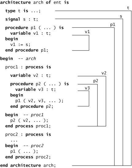
Figure 6.1 shows an outline of an architecture body of a model. It contains a number of declarations, including some procedure declarations. The visibility of each of the declarations is indicated. The first item to be declared is the type t; its visibility extends to the end of the architecture body. Thus it can be referred in other declarations, such as the variable declarations. The second declaration is the signal s; its visibility likewise extends to the end of the architecture body. So the assignment within procedure p1 is valid. The third and final declaration in the declarative part of the architecture body is that of the procedure p1, whose visibility extends to the end of the architecture body, allowing it to be called in either of the processes. It includes a local variable, v1, whose visibility extends only to the end of p1. This means it can be referred to in p1, as shown in the signal assignment statement, but neither process can refer to it.
In the statement part of the architecture body, we have two process statements, proc1 and proc2. The first includes a local variable declaration, v2, whose visibility extends to the end of the process body. Hence we can refer to v2 in the process body and in the procedure p2 declared within the process. The visibility of p2 likewise extends to the end of the body of proc1, allowing us to call p2 within proc1. The procedure p2 includes a local variable declaration, v3, whose visibility extends to the end of the statement part of p2. Hence we can refer to v3 in the statement part of p2. However, we cannot refer to v3 in the statement part of proc1, since it is not visible in that part of the model.
Finally, we come to the second process, proc2. The only items we can refer to here are those declared in the architecture body declarative part, namely, t, s and p1. We cannot call the procedure p2 within proc2, since it is local to proc1.
One point we mentioned earlier about subprograms but did not go into in detail was that we can include nested subprogram declarations within the declarative part of a subprogram. This means we can have local procedures and functions within a procedure or a function. In such cases, the simple rule for the visibility of a declaration still applies, so any items declared within an outer procedure before the declaration of a nested procedure can be referred to inside the nested procedure.
Example 6.24. Nested subprograms for memory read operations
The following is an outline of an architecture of a cache memory for a computer system.
   architecture behavioral of cache is
   begin
    behavior : process is
      ...
      procedure read_block( start_address : natural;
                            entry : out cache_block ) is
        variable memory_address_reg : natural;
        variable memory_data_reg : word;

        procedure read_memory_word is
        begin
          mem_addr <= memory_address_reg;
          mem_read <= '1';
          wait until mem_ack;
          memory_data_reg := mem_data_in;
          mem_read <= '0';
          wait until not mem_ack;
        end procedure read_memory_word;
      begin  -- read_block
        for offset in 0 to block_size - 1 loop
          memory_address_reg := start_address + offset;
          read_memory_word;
          entry(offset) := memory_data_reg;
        end loop;
      end procedure read_block;
    begin  -- behavior
       ...
      read_block( miss_base_address, data_store(entry_index) );
       ...
    end process behavior;
   end architecture behavioral;
The entity interface (not shown) includes ports named mem_addr, mem_ready, mem_ack and mem_data_in. The process behavior contains a procedure, read_block, which reads a block of data from main memory on a cache miss. It has the local variables memory_address_reg and memory_data_reg. Nested inside of this procedure is another procedure, read_memory_word, which reads a single word of data from memory. It uses the value placed in memory_address_reg by the outer procedure and leaves the data read from memory in memory_data_reg.
Now let us consider a model in which we have one subprogram nested inside another, and each declares an item with the same name as the other, as shown in Figure 6.2. Here, the first variable v is visible within all of the procedure p2 and the statement body of p1. However, because p2 declares its own local variable called v, the variable belonging to p1 is not directly visible where p2’s v is visible. We say the inner variable declaration hides the outer declaration, since it declares the same name. Hence the addition within p2 applies to the local variable v of p2 and does not affect the variable v of p1. If we need to refer to an item that is visible but hidden, we can use a selected name. For example, within p2 in Figure 6.2, we can use the name p1.v to refer to the variable v declared in p1. Although the outer declaration is not directly visible, it is visible by selection. An important point to note about using a selected name in this way is that it can only be used within the construct containing the declaration. Thus, in Figure 6.2, we can only refer to p1.v within p1. We cannot use the name p1.v to “peek inside” of p1 from places outside p1.
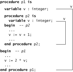
Figure 6.2. Nested procedures showing hiding of names. The declaration of v in p2 hides the variable v declared in p1.
The idea of hiding is not restricted to variable declarations within nested procedures. Indeed, it applies in any case where we have one declarative part nested within another, and an item is declared with the same name in each declarative part in such a way that the rules for resolving overloaded names are unable to distinguish between them. The advantage of having inner declarations hide outer declarations, as opposed to the alternative of simply disallowing an inner declaration with the same name, is that it allows us to write local procedures and processes without having to know the names of all items declared at outer levels. This is certainly beneficial when writing large models. In practice, if we are reading a model and need to check the use of a name in a statement against its declaration, we only need to look at successively enclosing declarative parts until we find a declaration of the name, and that is the declaration that applies.