
In this introductory chapter, we describe what we mean by digital system modeling and see why modeling and simulation are an important part of the design process. We see how the hardware description language VHDL can be used to model digital systems and introduce some of the basic concepts underlying the language. We complete this chapter with a description of the basic lexical and syntactic elements of the language, to form a basis for the detailed descriptions of language features that follow in later chapters.
If we are to discuss the topic of modeling digital systems, we first need to agree on what a digital system is. Different engineers would come up with different definitions, depending on their background and the field in which they were working. Some may consider a single VLSI circuit to be a self-contained digital system. Others might take a larger view and think of a complete computer, packaged in a cabinet with peripheral controllers and other interfaces.
For the purposes of this book, we include any digital circuit that processes or stores information as a digital system. We thus consider both the system as a whole and the various parts from which it is constructed. Therefore, our discussions cover a range of systems from the low-level gates that make up the components to the top-level functional units.
If we are to encompass this range of views of digital systems, we must recognize the complexity with which we are dealing. It is not humanly possible to comprehend such complex systems in their entirety. We need to find methods of dealing with the complexity, so that we can, with some degree of confidence, design components and systems that meet their requirements.
The most important way of meeting this challenge is to adopt a systematic methodology of design. If we start with a requirements document for the system, we can design an abstract structure that meets the requirements. We can then decompose this structure into a collection of components that interact to perform the same function. Each of these components can in turn be decomposed until we get to a level where we have some ready-made, primitive components that perform a required function. The result of this process is a hierarchically composed system, built from the primitive elements.
The advantage of this methodology is that each subsystem can be designed independently of others. When we use a subsystem, we can think of it as an abstraction rather than having to consider its detailed composition. So at any particular stage in the design process, we only need to pay attention to the small amount of information relevant to the current focus of design. We are saved from being overwhelmed by masses of detail.
We use the term model to mean our understanding of a system. The model represents that information which is relevant and abstracts away from irrelevant detail. The implication of this is that there may be several models of the same system, since different information is relevant in different contexts. One kind of model might concentrate on representing the function of the system, whereas another kind might represent the way in which the system is composed of subsystems. We will come back to this idea in more detail in the next section.
There are a number of important motivations for formalizing this idea of a model. First, when a digital system is needed, the requirements of the system must be specified. The job of the engineers is to design a system that meets these requirements. To do that, they must be given an understanding of the requirements, hopefully in a way that leaves them free to explore alternative implementations and to choose the best according to some criteria. One of the problems that often arises is that requirements are incompletely and ambiguously spelled out, and the customer and the design engineers disagree on what is meant by the requirements document. This problem can be avoided by using a formal model to communicate requirements.
A second reason for using formal models is to communicate understanding of the function of a system to a user. The designer cannot always predict every possible way in which a system may be used, and so is not able to enumerate all possible behaviors. If the designer provides a model, the user can check it against any given set of inputs and determine how the system behaves in that context. Thus a formal model is an invaluable tool for documenting a system.
A third motivation for modeling is to allow testing and verification of a design using simulation. If we start with a requirements model that defines the behavior of a system, we can simulate the behavior using test inputs and note the resultant outputs of the system. According to our design methodology, we can then design a circuit from subsystems, each with its own model of behavior. We can simulate this composite system with the same test inputs and compare the outputs with those of the previous simulation. If they are the same, we know that the composite system meets the requirements for the cases tested. Otherwise we know that some revision of the design is needed. We can continue this process until we reach the bottom level in our design hierarchy, where the components are real devices whose behavior we know. Subsequently, when the design is manufactured, the test inputs and outputs from simulation can be used to verify that the physical circuit functions correctly. This approach to testing and verification of course assumes that the test inputs cover all of the circumstances in which the final circuit will be used. The issue of test coverage is a complex problem in itself and is an active area of research.
A fourth motivation for modeling is to allow formal verification of the correctness of a design. Formal verification requires a mathematical statement of the required function of a system. This statement may be expressed in the notation of a formal logic system, such as temporal logic. Formal verification also requires a mathematical definition of the meaning of the modeling language or notation used to describe a design. The process of verification involves application of the rules of inference of the logic system to prove that the design implies the required function. While formal verification is not yet in everyday use, it is steadily becoming a more important part of the design process. There have already been significant demonstrations of formal verification techniques in real design projects, and the promise for the future is bright.
One final, but equally important, motivation for modeling is to allow automatic synthesis of circuits. If we can formally specify the function required of a system, it is in theory possible to translate that specification into a circuit that performs the function. The advantage of this approach is that the human cost of design is reduced, and engineers are free to explore alternatives rather than being bogged down in design detail. Also, there is less scope for errors being introduced into a design and not being detected. If we automate the translation from specification to implementation, we can be more confident that the resulting circuit is correct.
The unifying factor behind all of these arguments is that we want to achieve maximum reliability in the design process for minimum cost and design time. We need to ensure that requirements are clearly specified and understood, that subsystems are used correctly and that designs meet the requirements. A major contributor to excessive cost is having to revise a design after manufacture to correct errors. By avoiding errors, and by providing better tools for the design process, costs and delays can be contained.
In the previous section, we mentioned that there may be different models of a system, each focusing on different aspects. We can classify these models into three domains: function, structure and geometry. The functional domain is concerned with the operations performed by the system. In a sense, this is the most abstract domain of description, since it does not indicate how the function is implemented. The structural domain deals with how the system is composed of interconnected subsystems. The geometric domain deals with how the system is laid out in physical space.
Each of these domains can also be divided into levels of abstraction. At the top level, we consider an overview of function, structure or geometry, and at lower levels we introduce successively finer detail. Figure 1.1 (devised by Gajski and Kuhn, see reference [8]) represents the domains for digital systems on three independent axes and represents the levels of abstraction by the concentric circles crossing each of the axes.
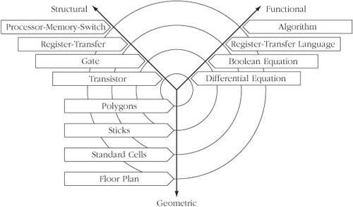
Figure 1.1. Domains and levels of abstraction. The radial axes show the three different domains of modeling. The concentric rings show the levels of abstraction, with the more abstract levels on the outside and more detailed levels toward the center.
Let us look at this classification in more detail, showing how at each level we can create models in each domain. As an example, we consider a single-chip microcontroller system used as the controller for some measurement instrument, with data input connections and some form of display outputs.
At the most abstract level, the function of the entire system may be described in terms of an algorithm, much like an algorithm for a computer program. This level of functional modeling is often called behavioral modeling, a term we shall adopt when presenting abstract descriptions of a system’s function. A possible algorithm for our instrument controller is shown below. This model describes how the controller repeatedly scans each data input and writes a scaled display of the input value.
   loop
    for each data input loop
      read the value on this input;
      scale the value using the current scale factor
        for this input;
      convert the scaled value to a decimal string;
      write the string to the display output corresponding
        to this input;
    end loop;
    wait for 10 ms;
   end loop;
At this top level of abstraction, the structure of a system may be described as an interconnection of such components as processors, memories and input/output devices. This level is sometimes called the Processor Memory Switch (PMS) level, named after the notation used by Bell and Newell (see reference [3]). Figure 1.2 shows a structural model of the instrument controller drawn using this notation. It consists of a processor connected via a switch to a memory component and to controllers for the data inputs and display outputs.
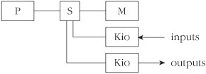
Figure 1.2. A PMS model of the controller structure. It is constructed from a processor (P), a memory (M), an interconnection switch (S) and two input/output controllers (Kio).
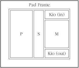
In the geometric domain at this top level of abstraction, a system to be implemented as a VLSI circuit may be modeled using a floor plan. This shows how the components described in the structural model are arranged on the silicon die. Figure 1.3 shows a possible floor plan for the instrument controller chip. There are analogous geometric descriptions for systems integrated in other media. For example, a personal computer system might be modeled at the top level in the geometric domain by an assembly diagram showing the positions of the motherboard and plug-in expansion boards in the desktop cabinet.
The next level of abstraction in modeling, depicted by the second ring in Figure 1.1, describes the system in terms of units of data storage and transformation. In the structural domain, this is often called the register-transfer level (RTL), composed of a data path and a control section. The data path contains data storage registers, and data is transferred between them through transformation units. The control section sequences operation of the data path components. For example, a register-transfer-level structural model of the processor in our controller is shown in Figure 1.4.
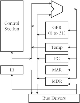
Figure 1.4. A register-transfer-level structural model of the controller processor. It consists of a generalpurpose register (GPR) file; registers for the program counter (PC), memory address (MAR), memory data (MDR), temporary values (Temp) and fetched instructions (IR); an arithmetic unit; bus drivers and the control section.
In the functional domain, a register-transfer language is often used to specify the operation of a system at this level. Storage of data is represented using register variables, and transformations are represented by arithmetic and logical operators. For example, an RTL model for the processor in our example controller might include the following description:
   MAR ← PC  memory_read ← 1
   PC ← PC + 1
   wait until ready = 1
   IR ← memory_data
   memory_read ← 0
This section of the model describes the operations involved in fetching an instruction from memory. The contents of the PC register are transferred to the memory address register, and the memory_read signal is asserted. Then the value from the PC register is transformed (incremented in this case) and transferred back to the PC register. When the ready input from the memory is asserted, the value on the memory data input is transferred to the instruction register. Finally, the memory_read signal is negated.
In the geometric domain, the kind of model used depends on the physical medium. In our example, standard library cells might be used to implement the registers and data transformation units, and these must be placed in the areas allocated in the chip floor plan.
The third level of abstraction shown in Figure 1.1 is the conventional logic level. At this level, structure is modeled using interconnections of gates, and function is modeled by Boolean equations or truth tables. In the physical medium of a custom integrated circuit, geometry may be modeled using a virtual grid, or “sticks,” notation.
At the most detailed level of abstraction, we can model structure using individual transistors, function using the differential equations that relate voltage and current in the circuit, and geometry using polygons for each mask layer of an integrated circuit. Most designers do not need to work at this detailed level, as design tools are available to automate translation from a higher level.
In the previous section, we saw that different kinds of models can be devised to represent the various levels of function, structure and physical arrangement of a system. There are also different ways of expressing these models, depending on the use made of the model.
As an example, consider the ways in which a structural model may be expressed. One common form is a circuit schematic. Graphical symbols are used to represent subsystems, and instances of these are connected using lines that represent wires. This graphical form is generally the one preferred by designers. However, the same structural information can be represented textually in the form of a net list.
When we move into the functional domain, we usually see textual notations used for modeling. Some of these are intended for use as specification languages, to meet the need for describing the operation of a system without indicating how it might be implemented. These notations are usually based on formal mathematical methods, such as temporal logic or abstract state machines. Other notations are intended for simulating the system for test and verification purposes and are typically based on conventional programming languages. Yet other notations are oriented toward hardware synthesis and usually have a more restricted set of modeling facilities, since some programming language constructs are difficult to translate into hardware.
The purpose of this book is to describe the modeling language VHDL. VHDL includes facilities for describing structure and function at a number of levels, from the most abstract down to the gate level. It also provides an attribute mechanism that can be used to annotate a model with information in the geometric domain. VHDL is intended, among other things, as a modeling language for specification and simulation. We can also use it for hardware synthesis if we restrict ourselves to a subset that can be automatically translated into hardware.
In Section 1.2, we looked at the three domains of modeling: function, structure and geometry. In this section, we look at the basic modeling concepts in each of these domains and introduce the corresponding VHDL elements for describing them. This will provide a feel for VHDL and a basis from which to work in later chapters.
Example 1.1. A four-bit register design
Figure 1.5 shows a schematic symbol for a four-bit register. Using VHDL terminology, we call the module reg4 a design entity, and the inputs and outputs are ports.
We write a VHDL description of the interface to this entity as follows:
   entity reg4 is
    port ( d0, d1, d2, d3, en, clk : in bit;
           q0, q1, q2, q3 : out  bit );
   end entity reg4;
This is an example of an entity declaration. It introduces a name for the entity and lists the input and output ports, specifying that they carry bit values (‘0’ or ‘1’) into and out of the entity. From this we see that an entity declaration describes the external view of the entity.
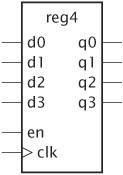
Figure 1.5. A four-bit register module. The register is named reg4 and has six inputs, d0, d1, d2, d3, en and clk, and four outputs, q0, q1, q2 and q3.
In VHDL, a description of the internal implementation of an entity is called an architecture body of the entity. There may be a number of different architecture bodies of the one interface to an entity, corresponding to alternative implementations that perform the same function. We can write a behavioral architecture body of an entity, which describes the function in an abstract way. Such an architecture body includes only process statements, which are collections of actions to be executed in sequence. These actions are called sequential statements and are much like the kinds of statements we see in a conventional programming language. The types of actions that can be performed include evaluating expressions, assigning values to variables, conditional execution, repeated execution and subprogram calls. In addition, there is a sequential statement that is unique to hardware modeling languages, the signal assignment statement. This is similar to variable assignment, except that it causes the value on a signal to be updated at some future time.
Example 1.2. Behavioral architecture for the four-bit register
To illustrate these ideas, let us look at a behavioral architecture body for the reg4 entity of Example 1.1:
   architecture behav of reg4 is
   begin
    storage : process is
      variable stored_d0, stored_d1, stored_d2, stored_d3 : bit;
    begin
      wait until clk;
      if en then
        stored_d0 := d0;
        stored_d1 := d1;
        stored_d2 := d2;
        stored_d3 := d3;
      end if;
      q0 <= stored_d0 after 5 ns;
      q1 <= stored_d1 after 5 ns;
      q2 <= stored_d2 after 5 ns;
      q3 <= stored_d3 after 5 ns;
    end process storage;
   end architecture behav;
In this architecture body, the part after the first begin keyword includes one process statement, which describes how the register behaves. It starts with the process name, storage, and finishes with the keywords end process.
The process statement defines a sequence of actions that are to take place when the system is simulated. These actions control how the values on the entity’s ports change over time; that is, they control the behavior of the entity. This process can modify the values of the entity’s ports using signal assignment statements.
The way this process works is as follows. When the simulation is started, the signal values are set to ‘0’, and the process is activated. The process’s variables (listed after the keyword variable) are initialized to ‘0’, then the statements are executed in order. The first statement is a wait statement that causes the process to suspend, that is, to become inactive. It stays suspended until one of the signals to which it is sensitive changes value. In this case, the process is sensitive only to the signal clk, since that is the only one named in the wait statement. When that signal changes value, the process is resumed and continues executing statements. The next statement is a condition that tests whether the value of the en signal is ‘1’. If it is, the statements between the keywords then and end if are executed, updating the process’s variables using the values on the input signals. After the conditional if statement, there are four signal assignment statements that cause the output signals to be updated 5 ns later.
When all of these statements in the process have been executed, the process starts again from the keyword begin, and the cycle repeats. Notice that while the process is suspended, the values in the process’s variables are not lost. This is how the process can represent the state of a system.
An alternative way of describing the implementation of an entity is to specify how it is composed of subsystems. We can give a structural description of the entity’s implementation. An architecture body that is composed only of interconnected subsystems is called a structural architecture body.
Example 1.3. Structural architecture for the four-bit register
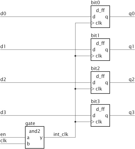
Figure 1.6 shows how the reg4 entity might be composed of flipflops and gates.
If we are to describe this in VHDL, we will need entity declarations and architecture bodies for the subsystems. For the flipflops, the entity and architecture are
   entity d_ff is
    port ( d, clk : in bit;  q : out bit );
   end d_ff;

   architecture basic of d_ff is
   begin

    ff_behavior : process is
    begin
      wait until clk;
      q <= d after 2 ns;
    end process ff_behavior;

   end architecture basic;
For the two-input and gate, the entity and architecture are
   entity and2 is
    port ( a, b : in bit;  y : out bit );
   end and2;

   architecture basic of and2 is
   begin

    and2_behavior : process is
    begin
      y <= a and b after 2 ns;
      wait on a, b;
    end process and2_behavior;

   end architecture basic;
We can now proceed to a VHDL architecture body declaration that describes the reg4 structure shown in Figure 1.6:
   architecture struct of reg4 is
    signal int_clk : bit;
   begin
    bit0 : entity work.d_ff(basic)
      port map (d0, int_clk, q0);
    bit1 : entity work.d_ff(basic)
      port map (d1, int_clk, q1);
    bit2 : entity work.d_ff(basic)
      port map (d2, int_clk, q2);
    bit3 : entity work.d_ff(basic)
      port map (d3, int_clk, q3);

    gate : entity work.and2(basic)
      port map (en, clk, int_clk);

   end architecture struct;
The signal declaration, before the keyword begin, defines the internal signals of the architecture. In this example, the signal int_clk is declared to carry a bit value (‘0’ or ‘1’). In general, VHDL signals can be declared to carry arbitrarily complex values. Within the architecture body the ports of the entity are also treated as signals.
In the second part of the architecture body, a number of component instances are created, representing the subsystems from which the reg4 entity is composed. Each component instance is a copy of the entity representing the subsystem, using the corresponding basic architecture body. (The name work refers to the current working library, in which all of the entity and architecture body descriptions are assumed to be held.)
The port map specifies the connection of the ports of each component instance to signals within the enclosing architecture body. For example, bit0, an instance of the d_ff entity, has its port d connected to the signal d0, its port clk connected to the signal int_clk and its port q connected to the signal q0.
Models need not be purely structural or purely behavioral. Often it is useful to specify a model with some parts composed of interconnected component instances, and other parts described using processes. We use signals as the means of joining component instances and processes. A signal can be associated with a port of a component instance and can also be assigned to or read in a process.
We can write such a hybrid model by including both component instance and process statements in the body of an architecture. These statements are collectively called concurrent statements, since the corresponding processes all execute concurrently when the model is simulated.
Example 1.4. A mixed structural and behavioral model for a multiplier
A sequential multiplier consists of a data path and a control section. An outline of a mixed structural and behavioral model for the multiplier is:
   entity multiplier is
    port ( clk, reset : in bit;
           multiplicand, multiplier : in integer;
           product : out integer );
   end entity multiplier;
   --------------------------------------------------
   architecture mixed of multiplier is

    signal partial_product, full_product : integer;
    signal arith_control, result_en, mult_bit, mult_load : bit;
   begin -- mixed
    arith_unit : entity work.shift_adder(behavior)
      port map ( addend => multiplicand, augend => full_product,
                 sum => partial_product,
                 add_control => arith_control);
    result : entity work.reg(behavior)
       port map ( d => partial_product, q => full_product,
                 en => result_en, reset => reset);
    multiplier_sr : entity work.shift_reg(behavior)
       port map ( d => multiplier, q => mult_bit,
                    load => mult_load, clk => clk);
    product <= full_product;
    control_section : process is
       -- variable declarations for control_section
       -- ...
    begin -- control section
       -- sequential statements to assign values to control signals
       -- ...
       wait on clk, reset;
    end process control_section;
   end architecture mixed;
The data path is described structurally, using a number of component instances. The control section is described behaviorally, using a process that assigns to the control signals for the data path.
In our introductory discussion, we mentioned testing through simulation as an important motivation for modeling. We often test a VHDL model using an enclosing model called a test bench. The name comes from the analogy with a real hardware test bench, on which a device under test is stimulated with signal generators and observed with signal probes. A VHDL test bench consists of an architecture body containing an instance of the component to be tested and processes that generate sequences of values on signals connected to the component instance. The architecture body may also contain processes that test that the component instance produces the expected values on its output signals. Alternatively, we may use the monitoring facilities of a simulator to observe the outputs.
Example 1.5. Test bench for the four-bit register
A test bench model for the behavioral implementation of the reg4 register is:
   entity test_bench is
   end entity test_bench;
   architecture test_reg4 of test_bench is
    signal d0, d1, d2, d3, en, clk, q0, q1, q2, q3 : bit;
   begin
    dut : entity work.reg4(behav)
      port map ( d0, d1, d2, d3, en, clk, q0, q1, q2, q3 );
    stimulus : process is
    begin
      d0 <= '1';  d1 <= '1';  d2 <= '1';  d3 <= '1';
      en <= '0';  clk <= '0';
      wait for 20 ns;
      en <= '1';  wait for 20 ns;
      clk <= '1';  wait for 20 ns;
      d0 <= '0';  d1 <= '0';  d2 <= '0';  d3 <= '0';  wait for 20 ns;
      en <= '0';  wait for 20 ns;
      ...
      wait;
    end process stimulus;
   end architecture test_reg4;
The entity declaration has no port list, since the test bench is entirely self-contained. The architecture body contains signals that are connected to the input and output ports of the component instance dut, the device under test. The process labeled stimulus provides a sequence of test values on the input signals by performing signal assignment statements, interspersed with wait statements. Each wait statement specifies a 20 ns pause during which the register device determines its output values. We can use a simulator to observe the values on the signals q0 to q3 to verify that the register operates correctly. When all of the stimulus values have been applied, the stimulus process waits indefinitely, thus completing the simulation.
One of the main reasons for writing a model of a system is to enable us to simulate it. This involves three stages: analysis, elaboration and execution. Analysis and elaboration are also required in preparation for other uses of the model, such as logic synthesis.
In the first stage, analysis, the VHDL description of a system is checked for various kinds of errors. Like most programming languages, VHDL has rigidly defined syntax and semantics. The syntax is the set of grammatical rules that govern how a model is written. The rules of semantics govern the meaning of a program. For example, it makes sense to perform an addition operation on two numbers but not on two processes.
During the analysis phase, the VHDL description is examined, and syntactic and static semantic errors are located. The whole model of a system need not be analyzed at once. Instead, it is possible to analyze design units, such as entity and architecture body declarations, separately. If the analyzer finds no errors in a design unit, it creates an intermediate representation of the unit and stores it in a library. The exact mechanism varies between VHDL tools.
The second stage in simulating a model, elaboration, is the act of working through the design hierarchy and creating all of the objects defined in declarations. The ultimate product of design elaboration is a collection of signals and processes, with each process possibly containing variables. A model must be reducible to a collection of signals and processes in order to simulate it.
We can see how elaboration achieves this reduction by starting at the top level of a model, namely, an entity, and choosing an architecture of the entity to simulate. The architecture comprises signals, processes and component instances. Each component instance is a copy of an entity and an architecture that also comprises signals, processes and component instances. Instances of those signals and processes are created, corresponding to the component instance, and then the elaboration operation is repeated for the subcomponent instances. Ultimately, a component instance is reached that is a copy of an entity with a purely behavioral architecture, containing only processes. This corresponds to a primitive component for the level of design being simulated. Figure 1.7 shows how elaboration proceeds for the structural architecture body of the reg4 entity from Example 1.3. As each instance of a process is created, its variables are created and given initial values. We can think of each process instance as corresponding to one instance of a component.
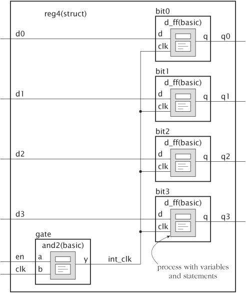
Figure 1.7. The elaboration of the reg4 entity using the structural architecture body. Each instance of the d_ff and and2 entities is replaced with the contents of the corresponding basic architecture. These each consist of a process with its variables and statements.
The third stage of simulation is the execution of the model. The passage of time is simulated in discrete steps, depending on when events occur. Hence the term discrete event simulation is used. At some simulation time, a process may be stimulated by changing the value on a signal to which it is sensitive. The process is resumed and may schedule new values to be given to signals at some later simulated time. This is called scheduling a transaction on that signal. If the new value is different from the previous value on the signal, an event occurs, and other processes sensitive to the signal may be resumed.
The simulation starts with an initialization phase, followed by repetitive execution of a simulation cycle. During the initialization phase, each signal is given an initial value, depending on its type. The simulation time is set to zero, then each process instance is activated and its sequential statements executed. Usually, a process will include a signal assignment statement to schedule a transaction on a signal at some later simulation time. Execution of a process continues until it reaches a wait statement, which causes the process to be suspended.
During the simulation cycle, the simulation time is first advanced to the next time at which a transaction on a signal has been scheduled. Second, all the transactions scheduled for that time are performed. This may cause some events to occur on some signals. Third, all processes that are sensitive to those events are resumed and are allowed to continue until they reach a wait statement and suspend. Again, the processes usually execute signal assignments to schedule further transactions on signals. When all the processes have suspended again, the simulation cycle is repeated. When the simulation gets to the stage where there are no further transactions scheduled, it stops, since the simulation is then complete.
When we learn a new natural language, such as Greek, Chinese or English, we start by learning the alphabet of symbols used in the language, then form these symbols into words. Next, we learn the way to put the words together to form sentences and learn the meaning of these combinations of words. We reach fluency in a language when we can easily express what we need to say using correctly formed sentences.
The same ideas apply when we need to learn a new special-purpose language, such as VHDL for describing digital systems. We can borrow a few terms from language theory to describe what we need to learn. First, we need to learn the alphabet with which the language is written. The VHDL alphabet consists of all of the characters in the ISO 8859 Latin-1 8-bit character set. This includes uppercase and lowercase letters (including letters with diacritical marks, such as “à”, “ä” and so forth), digits 0 to 9, punctuation and other special characters. Second, we need to learn the lexical elements of the language. In VHDL, these are the identifiers, reserved words, special symbols and literals. Third, we need to learn the syntax of the language. This is the grammar that determines what combinations of lexical elements make up legal VHDL descriptions. Fourth, we need to learn the semantics, or meaning, of VHDL descriptions. It is the semantics that allow a collection of symbols to describe a digital design. Fifth, we need to learn how to develop our own VHDL descriptions to describe a design we are working with. This is the creative part of modeling, and fluency in this part will greatly enhance our design skills.
In the remainder of this chapter, we describe the lexical elements used in VHDL and introduce the notation we use to describe the syntax rules. Then in subsequent chapters, we introduce the different facilities available in the language. For each of these, we show the syntax rules, describe the corresponding semantics and give examples of how they are used to model particular parts of a digital system. We also include some exercises at the end of each chapter to provide practice in the fifth stage of learning described above.
VHDL-87
VHDL-87 uses the ASCII character set, rather than the full ISO character set. ASCII is a subset of the ISO character set, consisting of just the first 128 characters. This includes all of the unaccented letters, but excludes letters with diacritical marks.
In the following section, we discuss the lexical elements of VHDL: comments, identifiers, reserved words, special symbols, numbers, characters, strings and bit strings.
When we are writing a hardware model in VHDL, it is important to annotate the code with comments. The reason for doing this is to help readers understand the structure and logic behind the model. It is important to realize that although we only write a model once, it may subsequently be read and modified many times, both by its author and by other engineers. Any assistance we can give to understanding the model is worth the effort. In this book, we set comments in slanted text to make them visually distinct.
A VHDL model consists of a number of lines of text. One form of comment, called a single-line comment, can be added to a line by writing two hypens together, followed by the comment text. For example:
... a line of VHDL code ... -- a descriptive commentThe comment extends from the two hyphens to the end of the line and may include any text we wish, since it is not formally part of the VHDL model. The code of a model can include blank lines and lines that only contain comments, starting with two hyphens. We can write long comments on successive lines, each line starting with two hyphens, for example:
   -- The following code models
   -- the control section of the system
   ... some VHDL code ...
Another form of comment, called a delimited comment, starts with the characters “/*” and extends to the closing characters “*/”. The opening and closing characters can be on different lines, or can be on the same line. Moreover, there can be further VHDL code on the line after the closing characters. Some examples are:
   /* This is a comment header that describes
     the purpose of the design unit. It contains
     all you ever wanted to know, plus more.
   */

   entity thingumy is
    port ( clk   : in bit; -- keeps it going
             reset : in bit /* start over */
             /* other ports to be added later */ );
   end entity thingumy;
Since the text in comments is ignored, it may contain comment delimiters. Mixing comment styles can be quite useful. For example, if we use delimited comments in a section of code, and we want to “comment out” the section, we can use single-line comments:
   -- This section commented out because it doesn't work
   -- /* Process to do a complicated computation
   -- involving lots of digital signal processing.
   -- */
   -- dsp_stuff : process is
   -- begin
   --   ...
   -- end process dsp_stuff;
However, we should be aware that comments do not nest. For example, the following is ill-formed:
   -- Here is the start of the comment: /* A comment extending
                                          over two lines */
The opening “/*” characters occur in a single-line comment, and so are ignored. Similarly, we cannot reliably use delimited comments to comment out a section of code, since the section might already contain a delimited comment:
   /* Comment out the following code:
   signal count_en : bit; /* counter enable */
   */
In this case, the occurrence of the characters “*/” on the second line closes the comment started on the first line, making the orphaned delimiter “*/” on the third line illegal. Provided we avoid pitfalls such as these, single-line and delimited comments are useful language features.
Identifiers are used to name items in a VHDL model. It is good practice to use names that indicate the purpose of the item, so VHDL allows names to be arbitrarily long. However, there are some rules about how identifiers may be formed. A basic identifier
may only contain alphabetic letters (‘A’ to ‘Z’ and ‘a’ to ‘z’), decimal digits (‘0’ to ‘9’) and the underline character (‘_’);
must start with an alphabetic letter;
may not end with an underline character; and
may not include two successive underline characters.
Some examples of valid basic identifiers are
A X0 counter Next_Value generate_read_cycle
Some examples of invalid basic identifiers are
   last@value     -- contains an illegal character for an identifier
   5bit_counter   -- starts with a non-alphabetic character
   _A0            -- starts with an underline
   A0_            -- ends with an underline
   clock__pulse   -- two successive underlines
Note that the case of letters is not considered significant, so the identifiers cat and Cat are the same. Underline characters in identifiers are significant, so This_Name and ThisName are different identifiers.
In addition to the basic identifiers, VHDL allows extended identifiers, which can contain any sequence of characters. Extended identifiers are included to allow communication between computer-aided engineering tools for processing VHDL descriptions and other tools that use different rules for identifiers. An extended identifier is written by enclosing the characters of the identifier between ‘’ characters. For example:
data bus global.clock 923 d#1 start__
If we need to include a ‘’ character in an extended identifier, we do so by doubling the character, for example:
A:\name -- contains a '' between the ':' and the 'n'Note that the case of letters is significant in extended identifiers and that all extended identifiers are distinct from all basic identifiers. So the following are all distinct identifiers:
   name
ame Name NAME
Some identifiers, called reserved words or keywords, are reserved for special use in VHDL. They are used to denote specific constructs that form a model, so we cannot use them as identifiers for items we define. The full list of reserved words is shown in Table 1.1. Often, when a VHDL program is typeset, reserved words are printed in boldface. This convention is followed in this book.
Table 1.1. VHDL reserved words
|
|
|
|
|
|
|
|
|
|
|
|
|
|
|
|
|
|
| |
|
|
|
|
|
|
|
|
| |
|
|
|
| |
|
|
|
|
|
|
|
|
| |
|
|
| ||
|
|
|
|
|
|
|
|
| |
|
|
|
| |
|
|
|
|
|
|
|
|
|
|
|
|
| ||
|
|
|
| |
|
|
|
|
|
|
|
|
| |
|
|
|
|
|
|
|
|
| |
|
|
|
| |
|
|
| ||
|
|
|
| |
|
|
|
| |
|
|
| ||
|
| |||
|
| |||
|
VHDL-2002
The following identifiers are not used as reserved words in VHDL-2002. They may be used as identifiers for other purposes, although it is not advisable to do so, as this may cause difficulties in porting the models to VHDL-2008.
   assert                 fairness        restrict_guarantee
   assume                 force           sequence
   assume_guarantee       parameter       strong
   context                property        vmode
   cover                  release         vprop
   default                restrict        vunit
VHDL uses a number of special symbols to denote operators, to delimit parts of language constructs and as punctuation. Some of these special symbols consist of just one character. They are
" # & ' ( ) * + - , . / : ; < = > ? @ [ ] ` |
Other special symbols consist of pairs of characters. The two characters must be typed next to each other, with no intervening space. These symbols are
=> ** := /= >= <= <> ?? ?= ?/= ?> ?< ?>= ?<= << >>
There are two forms of numbers that can be written in VHDL code: integer literals and real literals. An integer literal simply represents a whole number and consists of digits without a decimal point. Real literals, on the other hand, can represent fractional numbers. They always include a decimal point, which is preceded by at least one digit and followed by at least one digit. Real literals represent an approximation to real numbers.
Some examples of decimal integer literals are
23 0 146
Note that –10, for example, is not an integer literal. It is actually a combination of a negation operator and the integer literal 10.
Some examples of real literals are
23.1 0.0 3.14159
Both integer and real literals can also use exponential notation, in which the number is followed by the letter ‘E’ or ‘e’, and an exponent value. This indicates a power of 10 by which the number is multiplied. For integer literals, the exponent must not be negative, whereas for real literals, it may be either positive or negative. Some examples of integer literals using exponential notation are
46E5 1E+12 19e00
Some examples of real literals using exponential notation are
1.234E09 98.6E+21 34.0e-08
Integer and real literals may also be expressed in a base other than base 10. In fact, the base can be any integer between 2 and 16. To do this, we write the number surrounded by sharp characters (‘#’), preceded by the base. For bases greater than 10, the letters ‘A’ through ‘F’ (or ‘a’ through ‘f’) are used to represent the digits 10 through 15. For example, several ways of writing the value 253 are as follows:
2#11111101# 16#FD# 16#0fd# 8#0375#
Similarly, the value 0.5 can be represented as
2#0.100# 8#0.4# 12#0.6#
Note that in all these cases, the base itself is expressed in decimal.
Based literals can also use exponential notation. In this case, the exponent, expressed in decimal, is appended to the based number after the closing sharp character. The exponent represents the power of the base by which the number is multiplied. For example, the number 1024 could be represented by the integer literals:
2#1#E10 16#4#E2 10#1024#E+00
Finally, as an aid to readability of long numbers, we can include underline characters as separators between digits. The rules for including underline characters are similar to those for identifiers; that is, they may not appear at the beginning or end of a number, nor may two appear in succession. Some examples are
123_456 3.141_592_6 2#1111_1100_0000_0000#
A character literal can be written in VHDL code by enclosing it in single quotation marks. Any of the printable characters in the standard character set (including a space character) can be written in this way. Some examples are
   'A'   -- uppercase letter
   'z'   -- lowercase letter
   ','   -- the punctuation character comma
   '''   -- the punctuation character single quote
   ' '   -- the separator character space
A string literal represents a sequence of characters and is written by enclosing the characters in double quotation marks. The string may include any number of characters (including zero), but it must fit entirely on one line. Some examples are
   "A string"
   "A string can include any printing characters (e.g., &%@∧*)."
   "00001111ZZZZ"
   ""  -- empty string
If we need to include a double quotation mark character in a string, we write two double quotation mark characters together. The pair is interpreted as just one character in the string. For example:
"A string in a string: ""A string"". "
If we need to write a string that is longer than will fit on one line, we can use the concatenation operator (“&”) to join two substrings together. (This operator is discussed in Chapter 4.) For example:
   "If a string will not fit on one line, "
   & "then we can break it into parts on separate lines."
VHDL includes values that represent bits (binary digits), which can be either ‘0’ or ‘1’. A bit-string literal represents a string of these bit values. It is represented by a string of digits, enclosed by double quotation marks and preceded by a character that specifies the base of the digits. The base specifier can be one of the following:
B for binary,
O for octal (base 8) and
X for hexadecimal (base 16).
D for decimal (base 10).
For example, some bit-string literals specified in binary are
B"0100011" B"10" b"1111_0010_0001" B""
Notice that we can include underline characters in bit-string literals to separate adjacent digits. The underline characters do not affect the meaning of the literal; they simply make the literal more readable. The base specifier can be in uppercase or lowercase. The last of the examples above denotes an empty bit string.
If the base specifier is octal, the digits ‘0’ through ‘7’ can be used. Each digit represents exactly three bits in the bit string. Some examples are
   O"372"  -- equivalent to B"011_111_010"
   o"00"   -- equivalent to B"000_000"
If the base specifier is hexadecimal, the digits ‘0’ through ‘9’ and ‘A’ through ‘F’ or ‘a’ through ‘f’ (representing 10 through 15) can be used. In hexadecimal, each digit represents exactly four bits. Some examples are
   X"FA"   -- equivalent to B"1111_1010"
   x"0d"   -- equivalent to B"0000_1101"
Notice that O“372” is not the same as X“FA”, since the former is a string of nine bits, whereas the latter is a string of eight bits.
If the base specifier is decimal, the digits ‘0’ through ‘9’ can be used. The digits in the literal are interpreted as a decimal number and are converted to the equivalent binary value. The number of bits in the string is the minimal number needed to represent the value. Some examples are
   D"23"      -- equivalent to B"10111"
   D"64"      -- equivalent to B"1000000"
   D"0003"   -- equivalent to B"11"
In some cases, it is convenient to include characters other than digits in bit string literals. As we will see later, many VHDL models use characters such as ‘Z’, ‘X’, and ‘-’ to represent high-impedance states, unknown values, and don’t-care conditions. Models may use other characters for similar purposes. We can include such non-binary characters in bit-string literals. In an octal literal, any non-octal-digit character is expanded to three occurrences of that character in the bit string. Similarly, in a hexadecimal literal any non-hexadecimal-digit character is expanded to four occurrences of the character. In a binary literal, any non-bit character just represents itself in the vector. Some examples are:
   O"3XZ4"   -- equivalent to B"011XXXZZZ100"
   X"A3--"   -- equivalent to B"10100011--------"
   X"0#?F"   -- equivalent to B"0000####????1111"
   B"00UU"   -- equivalent to B"00UU"
While allowing this for binary literals might seem vacuous at first, the benefit will become clear shortly. Note that expansion of non-digit characters does not extend to embedded underscores, which we might add for readability. Thus, O“3_X” represents “011XXX”, not “011___XXX”. Also, non-digit characters are not allowed in decimal literals, since it would be unclear which bits of the resulting string correspond to the non-digit characters. Thus, the literal D“23Z9” is illegal.
In all of the preceding cases, the number of bits in the string is determined from the base specifier and the number of characters in the literal. We can, however, specify the exact length of bit string that we require from a literal. This allows us to specify strings whose length is not a multiple or three (for octal) or four (for hexadecimal). We do so by writing the length immediately before the base specifier, with no intervening space. Some examples are:
   7X"3C"   -- equivalent to B"0111100"
   8O"5"    -- equivalent to B"00000101"
   10B"X"   -- equivalent to B"000000000X"
If the final length of the string is longer than that implied by the digits, the string is padded on the left with ‘0’ bits. If the final length is less than that implied by the digits, the left-most elements of the string are truncated, provided they are all ‘0’. An error occurs if any non-‘0’ bits are truncated, as they would be in the literal 8X“90F”.
A further feature of bit-string literals is provision for specifying whether the literal represents an unsigned or signed number. We represent an unsigned number using one of the base specifiers UB, UO, or UX. These are the same as the ordinary base specifiers B, O, and X. When a sized unsigned literal is extended, it is padded with ‘0’ bits, and when bits are truncated, they must be all ‘0’. Decimal literals are always interpreted as unsigned, so D is the only base specifier for decimal. We can extend a decimal literal by padding with ‘0’ bits. However, we cannot truncate a decimal literal from its default size, since the default size always gives a ‘1’ as the leftmost bit, which must not be truncated.
We represent a signed number using one of the base specifiers SB, SO, or SX. The rules for extension and truncation are based on those for sign extension and truncation of 2s-complement binary numbers. When a sized signed literal is extended, each bit of padding on the left is a replication of the leftmost bit prior to padding. For example:
   10SX"71"   -- equivalent to B"0001110001"
   10SX"88"   -- equivalent to B"1110001000"
   10SX"W0"   -- equivalent to B"WWWWWW0000"
When a sized signed literal is truncated, all of the bits removed at the left must be the same as the leftmost remaining bit. For example:
   6SX"16"   -- equivalent to B"010110"
   6SX"E8"   -- equivalent to B"101000"
   6SX"H3"   -- equivalent to B"HH0011"
However, 6SX“28” is invalid, since, prior to truncation, the bit string would be “00101000”. The two leftmost bits removed are each ‘0’, which differ from the leftmost remaining ‘1’ bit. The literal would have to be written as 6SX“E8” for this reason. The rationale for this rule is that it prevents the signed numeric value represented by the literal being inadvertently changed by the truncation.
VHDL-87, -93, and -2002
These versions of VHDL only allow the base specifiers B, O, and X. They do not allow unsigned and signed specifiers UB, UO, UX, SB, SO, and SX; nor do they allow the decimal specifier D. They do not allow the size to be specified; thus, octal literals are always a multiple of three in length, and hexidecimal literals are always a multiple of four in length. Finally, non-digit characters, other than underlines for readability, are not allowed.
In the remainder of this book, we describe rules of syntax using a notation based on the Extended Backus-Naur Form (EBNF). These rules govern how we may combine lexical elements to form valid VHDL descriptions. It is useful to have a good working knowledge of the syntax rules, since VHDL analyzers expect valid VHDL descriptions as input. The error messages they otherwise produce may in some cases appear cryptic if we are unaware of the syntax rules.
The idea behind EBNF is to divide the language into syntactic categories. For each syntactic category we write a rule that describes how to build a VHDL clause of that category by combining lexical elements and clauses of other categories. These rules are analogous to the rules of English grammar. For example, there are rules that describe a sentence in terms of a subject and a predicate, and that describe a predicate in terms of a verb and an object phrase. In the rules for English grammar, “sentence”, “subject”, “predicate”, and so on, are the syntactic categories.
In EBNF, we write a rule with the syntactic category we are defining on the left of a “⇐” sign (read as “is defined to be”), and a pattern on the right. The simplest kind of pattern is a collection of items in sequence, for example:
variable_assignment ⇐ target:= expression ;
This rule indicates that a VHDL clause in the category “variable_assignment” is defined to be a clause in the category “target”, followed by the symbol “:=”, followed by a clause in the category “expression”, followed by the symbol “;”. To find out whether the VHDL clause
d0 := 25 + 6;
is syntactically valid, we would have to check the rules for “target” and “expression”. As it happens, “d0” and “25+6” are valid subclauses, so the whole clause conforms to the pattern in the rule and is thus a valid variable assignment. On the other hand, the clause
25 fred := x if := .
cannot possibly be a valid variable assignment, since it doesn’t match the pattern on the right side of the rule.
The next kind of rule to consider is one that allows for an optional component in a clause. We indicate the optional part by enclosing it between the symbols “[” and “]”. For example:
function_call ⇐ name [( association_list )]
This indicates that a function call consists of a name that may be followed by an association list in parentheses. Note the use of the outline symbols for writing the pattern in the rule, as opposed to the normal solid symbols that are lexical elements of VHDL.
In many rules, we need to specify that a clause is optional, but if present, it may be repeated as many times as needed. For example, in this simplified rule for a process statement:
   process_statement ⇐
        process is
            { process_declarative_item }
          begin
            { sequential_statement }
       end process ;
the curly braces specify that a process may include zero or more process declarative items and zero or more sequential statements. A case that arises frequently in the rules of VHDL is a pattern consisting of some category followed by zero or more repetitions of that category. In this case, we use dots within the braces to represent the repeated category, rather than writing it out again in full. For example, the rule
   case_statement ⇐
     case expression is

     case_statement_alternative
     { ... }
   end case ;
indicates that a case statement must contain at least one case statement alternative, but may contain an arbitrary number of additional case statement alternatives as required. If there is a sequence of categories and symbols preceding the braces, the dots represent only the last element of the sequence. Thus, in the example above, the dots represent only the case statement alternative, not the sequence “case expression is case_statement_alternative”.
We also use the dots notation where a list of one or more repetitions of a clause is required, but some delimiter symbol is needed between repetitions. For example, the rule
identifier_list ⇐ identifier { ,... }specifies that an identifier list consists of one or more identifiers, and that if there is more than one, they are separated by comma symbols. Note that the dots always represent a repetition of the category immediately preceding the left brace symbol. Thus, in the above rule, it is the identifier that is repeated with comma delimiters; it is not just the comma that is repeated.
Many syntax rules allow a category to be composed of one of a number of alternatives. One way to represent this is to have a number of separate rules for the category, one for each alternative. However, it is often more convenient to combine alternatives using the “│” symbol. For example, the rule
mode ⇐ in | out | inout
specifies that the category “mode” can be formed from a clause consisting of one of the reserved words chosen from the alternatives listed.
The final notation we use in our syntax rules is parenthetic grouping, using the symbols “(“ and “)”. These simply serve to group part of a pattern, so that we can avoid any ambiguity that might otherwise arise. For example, the inclusion of parentheses in the rule
term ⇐ factor {( * | / | mod | rem ) factor }makes it clear that a factor may be followed by one of the operator symbols, and then another factor. Without the parentheses, the rule would be
term ⇐ factor {* | / | mod | rem factor }indicating that a factor may be followed by one of the operators “*”, “/” or mod alone, or by the operator rem and then another factor. This is certainly not what is intended. The reason for this incorrect interpretation is that there is a precedence, or order of priority, in the EBNF notation we are using. In the absence of parentheses, a sequence of pattern components following one after the other is considered as a group with higher precedence than components separated by “│” symbols.
This EBNF notation is sufficient to describe the complete grammar of VHDL. However, there are often further constraints on a VHDL description that relate to the meaning of the lexical elements used. For example, a description specifying connection of a signal to a named object that identifies a component instead of a port is incorrect, even though it may conform to the syntax rules. To avoid such problems, many rules include additional information relating to the meaning of a language feature. For example, the rule shown above describing how a function call is formed is augmented thus:
function_call ⇐ function_name [ ( parameter_association_list ) ]The italicized prefix on a syntactic category in the pattern simply provides semantic information. This rule indicates that the name cannot be just any name, but must be the name of a function. Similarly, the association list must describe the parameters supplied to the function. (We will describe the meaning of functions and parameters in a later chapter.) The semantic information is for our benefit as designers reading the rule, to help us understand the intended semantics. So far as the syntax is concerned, the rule is equivalent to the original rule without the italicized parts.
In the following chapters, we will introduce each new feature of VHDL by describing its syntax using EBNF rules, and then we will describe the meaning and use of the feature through examples. In many cases, we will start with a simplified version of the syntax to make the description easier to learn and come back to the full details in a later chapter. For reference, Appendix Bcontains a complete listing of VHDL syntax in EBNF notation.
[ | |
[ apply_transform : process is begin d_out <= transform(d_in) after 200 ps; debug_test <= transform(d_in); wait on enable, d_in; end process apply_transform; | |
[ last_item prev item value-1 buffer element#5 _control 93_999 entry_ | |
[ 1 34 256.0 0.5 | |
[ 8#14# 2#1000_0100# 16#2C# 2.5E5 2#1#E15 2#0.101# | |
[ | |
[ O"747" O"377" O"1_345" X"F2" X"0014" X"0000_0001" | |
[ 10UO"747" 10UO"377" 10UO"1_345" 10SO"747" 10SO"377" 10SO"1_345" 12UX"F2" 12SX"F2" 10UX"F2" 10SX"F2" | |
[ D"24" 12D"24" 4D"24" | |
10. | [ |
11. | [ |