Step 1 Defining operating free cash flow

So what is operating free cash flow? This is normally defined as:

Depreciation and amortisation are added back as they are what are called ‘non-cash costs’. This means that while the amounts are deducted to arrive at a profit number, they do not involve an outflow of cash.

Capital expenditure explicitly recognises that this is a critical component of the company achieving the forecast growth targets. Maintenance capital expenditure is often used in more slowly growing environments or phases of a company’s development. This ensures that the fabric of the business is protected, recognising that maintenance expenditure is a real cost of doing business (a weakness discussed when considering EBITDA as a valuation number).

Similarly, working capital is required as the higher sales over the growth period will require cash to fund the expansion of working capital.

Things to watch out for include:

• Is cash coming from the underlying business and is it sustainable? While this seems an obvious point, it is always worth ensuring that the cash is coming from the business and is sustainable. A one-off movement in working capital that improves the cash flow profile may unwind in another year.
• How much is from one-offs (e.g. asset disposals)? There may be one-offs coming from asset or business disposals which again need to be excluded or considered separately.
• Associate income. As we discussed when exploring earnings quality and cash flows, it is important that associate income is excluded. In cash flow terms this generates a dividend. Often it is best to exclude this contribution and deduct a value for the associate from the enterprise value (treating it as a ‘peripheral asset’, see p. 275).
• Minorities. Again as discussed under earnings, if a part of the business is owned by outside shareholders this also needs to be considered.

Step 2 Forecasting cash flow

The initial period of forecasting is typically between five and ten years. The key variables driving operating cash flow, prices and volumes (which drive revenues) and costs need to be forecast and the relationship between these variables really need to be understood – so, for example, how does a fall in price affect operating profit?

As the section on the difficulties of forecasting made clear (p. 222), this is a hazardous process fraught with difficulties even in the short term, let alone the long term.

The frequency and extent of profits downgrades that have afflicted the stock market clearly demonstrate the risks and difficulties in forecasting. Interestingly, during the dot-com boom many of the downgrades have been in perceived growth stocks (e.g. telecommunications or technology) where DCF may well have been used to justify their share price/value. In the current environment the lack of visibility for many highly cyclical business makes for a real challenge using DCF.

Therefore, when forecasting this initial period, care needs to be taken with the following.

• Forecasting volumes, prices and costs. As these are the key drivers of cash, great care must be taken arriving at the forecasts. The section on the difficulties of forecasting volumes, prices and costs (p. 222) explores the issues and problems at the heart of this element of a DCF valuation. The impact of operational gearing and the sensitivity of profits and cash flow to changes in price are especially crucial. Also really appreciating the company’s competitive position and ‘moat’ are crucial to have confidence in the sustainability of the projections and ability to prevent or withstand new entrants.
• ’Sanity checks’ – do the forecasts make sense? The level of volumes, prices and costs should be subject to a ‘sanity check’ so that any overoptimistic assumptions are reined in. Are the volume forecasts predicated on taking a degree of market share that will inevitably cause a price war? Are volume assumptions extrapolated on the back of high and unsustainable current levels? Are prices likely to come under pressure from new entrants or customers with strong bargaining power? Are the operating margins realistic in the context of the economics of the industry? Again, it is important to be sceptical of any forecasts used.
• How long is the growth period? Over the initial forecast period the company is often in a high-growth phase. This period of high growth and high returns will tend to decay as the company becomes more established. At some stage demand growth slows and increasingly competitive conditions arise affecting growth and returns. The length of this initial period of strong growth and returns is of course subject to considerable uncertainty. In many new industries the growth periods may be a lot shorter than hoped for as maturity quickly follows a period of exceptional growth. Clearly if the industry matures in Year 5 and the forecasts of exceptional growth go out to Year 8, the valuation will fall sharply.

In theory, at the end of the initial growth period returns will fall until the cost of capital is covered. When the company has arrived at this phase of its development, at the end of the initial forecast period, the valuation process turns to the terminal value phase.

Step 3 Terminal value

The terminal value is often 50–60 per cent of the total value of the company. Making appropriate assumptions at this stage of the company’s development is therefore crucial. Indeed, flexing the assumptions at this stage can be used to generate a very different result (see p. 172).

There are two ways of determining the terminal value. First, a multiple of the operating profits or operating free cash flow can be used. Alternatively a ‘steady state growth’ approach can be used.

• A multiple approach. With a multiple approach you would take (say) the operating profits at this stage and apply a multiple. Let’s say the company is forecast to be generating operating profits of £50 million. Having looked at similar companies with these characteristics and growth profile, you find they are trading on 73 operating profit. You simply multiply the £50 million by 7 to generate the terminal value of £350 million. This then has to be discounted back to the current value. If the terminal value occurs in, say, Year 7, you would discount back from Year 7.
• The danger, arguably, of using the multiple method is that the absolute nature of using the DCF approach is compromised by using the relative valuation implied by the multiple. It raises questions as to what multiple should be used given the low-growth scenario at this stage of the company’s development.
• Steady state growth. The ‘steady state’ refers to the maturity of the business and implicitly relatively low-growth assumptions should be used. When projecting growth at the terminal phase in a steady state approach, it may be sensible to tie the assumptions to the long-term trend in GDP growth.
• There is a formula that can be used to determine the terminal value based on something called the ‘Gordon growth model’. We will not go into the basis for this here but the formula is really useful.

• In this case the drivers of value are the cost of capital and the assumed growth rates. The higher the growth rate, the greater the value as you are dividing the operating profit by a much lower figure.
• The sum generated by this formula is then discounted back from the last forecast period. So again if you have forecast out to Year 7, the terminal value will be discounted back from Year 7.

We now need to assess the cost of capital and how to derive the weighted average cost of capital.

Step 4 The weighted average cost of capital (WACC)

Having decided upon the forecasts for the initial growth phase and the assumptions used for the terminal value phase, the cash flows need to be ‘discounted’. This means that the future value of the cash is brought back to a current value, what the cash flows are worth in today’s money. This is why the calculation is often referred to as a ‘net present value’ calculation. The further away the cash is and the greater the risk attaching to it the less it is worth in today’s money.

In essence the discount rate will reflect how much risk attaches to the future cash flows – how predictable are the price, volume and cost elements of the equation and how volatile are profits? So the higher the perceived risk the greater the WACC. A biotech company, for example, may have a 25 per cent discount rate while with a utility with a predictable cash flow stream we may use a rate of 6 per cent.

The discount rate used is the WACC and how it is calculated was discussed in Chapter 1 (p. 27). The key element determining the WACC is the proportion of equity and debt used to fund the business. Here we use the market values (if possible) of the equity (market cap) and debt. Equity – as it is higher risk – has a much higher cost than debt (which is also tax deductible).

Step 5 The calculation

To illustrate the way in which the discounted cash flow process works we return to our two fictional companies, pharmaceutical stock Pink Tablet and manufacturing Tin Can. We shall explore the mechanics of the DCF valuation and assess how this valuation method compares with the others.

The operating forecasts are detailed in Tables 7.1 and 7.2.

Table 7.1 Pink Tablet operating forecasts

The process involves:

• defining operating free cash flow
• looking at the initial growth period
• assessing terminal value
• WACC
• the calculation.

Defining operating free cash flow

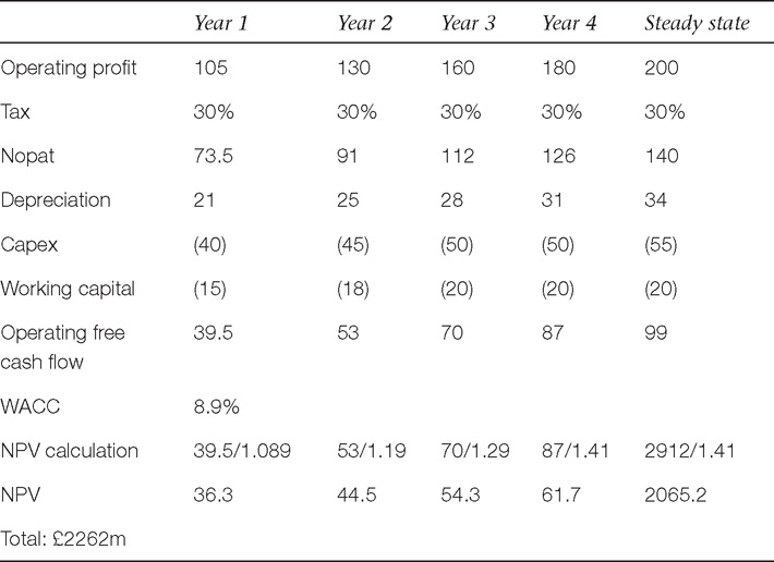
Table 7.1 lays out the components of operating free cash flow for Pink Tablet. The operating profit is taxed at 30 per cent. Depreciation as a non-cash cost is added back on. We then have to deduct the amount spent on capital expenditure. In this case it is relatively modest as, for pharmaceutical companies, it is the R&D budget that is the major area of investment and this is charged to costs as a revenue item. Then working capital requirements are deducted. This leaves us with the operational free cash flow.

Initial growth period

We have forecast operating profits out for the first four years. The growth rate is very high in the first two years in particular, with operating profit growing at 23 per cent per annun. This reflects the success of drugs that have reached the market in year 1 and built up sales in their first two years. This slows down in year 4. For the sake of illustration we have restricted this initial growth period to the first four years. It will often be the case that the initial period will be for the first seven to ten years. Obviously the risks attaching to the numbers when forecasting out so far increase dramatically.

Terminal value – steady state growth phase

At the end of Year 4 it is assumed that the steady state growth rate slows considerably. The steady state represents an 11 per cent uplift on Year 4. Thereafter it is assumed that the growth rate at this stage falls to 5.5 per cent. This is considerably above the growth rate of the economy (which for the sake of argument grows at a long-term rate of 2.5 per cent).

We will use the formula:

We then need to establish the WACC.

Weighted average cost of capital

Cost of debt: we already know that Pink Tablet is very low geared and highly cash generative. As a result it can borrow money very cheaply. We will assume that it pays 6.5 per cent on its debt. Given that interest payments are tax deductible, the net cost of debt is 70 per cent of 6.5 per cent – or 4.6 per cent.

Cost of equity: we know that for a pharmaceutical company the impact of the economy on operating results is relatively low, the operational gearing is relatively low and the company is very low geared (it has little debt). The impact of the economy on operating results is relatively low. As a result the beta of the shares is going to be low. We will use 0.7 – consistent with pharmaceutical shares in the market.

If we take the risk-free rate on a long-term government bond as being 5.5 per cent and a relatively high equity risk premium of 5 per cent given the uncertainty of the current environment then:

The mix of equity and debt is very much skewed towards equity. The market capitalisation is £2415 million, while there is debt of £50 million. This gives a business 98 per cent funded by equity and 2 per cent by debt.

Therefore the WACC is:

The calculation

We are now in a position to calculate the DCF of Pink Tablet. The discounting process works as we have seen by dividing the operating free cash flow by 1 plus the WACC with this is factored by the relevant number. The formula is normally expressed as:

Table 7.1 demonstrates how the numbers are put together. The series for the initial growth period runs:

Using the formula, the terminal value is 99/(8.9 per cent – 5.5 per cent) = 2912. As this is the value at the end of Year 4 we then have to discount this back to obtain a net present value. Discounting this back from the end of Year 4, i.e. £2912 million/(1.089)4, gives us £2065.2 million.

This value is the value of the whole business, the enterprise value. To arrive at the value of the shares we have to take the debt off this amount to generate the equity value. Therefore on this basis the equity value is £2262 million – £50 million = £2212 million.

From the market capitalisation, we know that the stock market values the shares at £2415 million. Therefore we can say that the DCF is producing a value 8.5 per cent below that of the company’s stock market value. On this basis, if we believe all our numbers and projections, we would conclude that the shares are overvalued. Alternatively, we can argue that the stock market is making more optimistic assumptions than our central case.

To illustrate the sensitivities involved, if we flex the terminal growth assumption to 6 per cent (feasible given the growth profile of a drug company), the terminal value becomes £3414 million; discounted back this is £2421.2 million: a £356 million uplift on the original valuation. This gives an equity value of £2568 million, 6 per cent more than the price of the shares.

Flexing the steady state growth assumption by 0.5 per cent equates to the shares going from being 8.5 per cent dear to 6 per cent cheap.

Table 7.2 Tin Can operating forecasts

Once again the process is as follows:

• defining operating free cash flow
• looking at the initial growth period
• assessing terminal value
• WACC
• the calculation.

Defining operating free cash flow

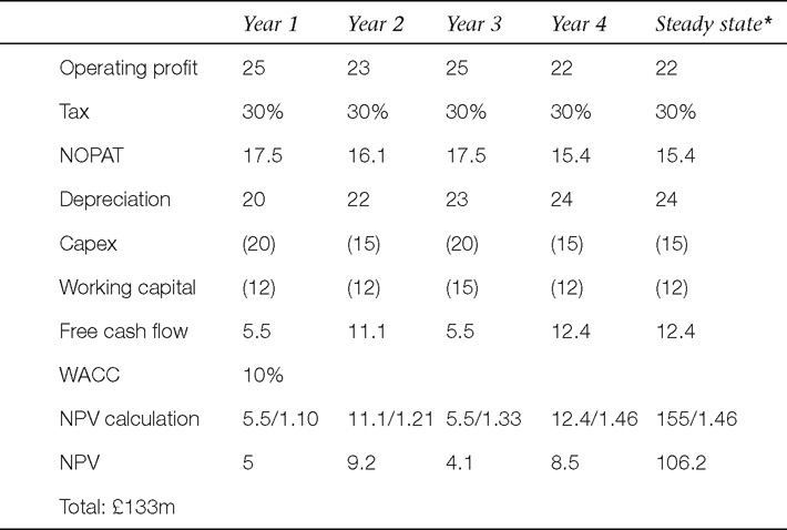
Table 7.2 lays out the components of operating free cash flow for Tin Can. The operating profit is taxed at 30 per cent. Depreciation as a non-cash cost is added back on. We then have to deduct the amount spent on capital expenditure. In this case we have assumed that maintenance capital expenditure is £15 million, £5 million below depreciation.

Initial growth period

We have forecast operating profits out for the first four years. For the sake of illustration, we have restricted this initial growth period to the first four years. It will often be the case that the initial period will be for the first seven to ten years. Obviously the risks attaching to the numbers when forecasting out so far increase dramatically.

The forecasts reflect the cyclicality of the markets and the non-existent growth prospects.

Terminal value – steady state growth phase

At the end of Year 4 it is assumed that the steady state growth rate slows considerably. The steady state is unchanged in Year 4. Thereafter it is assumed that the growth rate falls to 2 per cent. This is in line with the growth rate of the economy (which for the sake of argument grows at a long-term rate of 2.5 per cent). This could be a little optimistic given the characteristics of the business.

To generate the terminal value we will use the formula:

We then need to establish the WACC.

Weighted average cost of capital

Cost of debt: we already know that Tin Can is highly geared and there are question marks over its cash generation. However, it has locked in long-term loan rates at an attractive 7.5 per cent.

Cost of equity: we know that Tin Can is very sensitive to changes in volumes and pricing (which is highly competitive and subject to import competition) and so operational gearing is high. With 50 per cent gearing the company is also highly financially geared. As a result the beta of the shares is going to be high. We will use 1.3 (which is reasonably consistent with engineering shares in the market).

If we take the risk-free rate on a long-term government bond as being 5.5 per cent and a relatively high equity risk premium of 5 per cent given the uncertainty of the current environment then the cost of equity is:

The market capitalisation is £138 million, while there is debt of £60 million. This gives a business funded 70 per cent by equity and 30 per cent by debt.

Therefore the WACC is:

The calculation

We are now in a position to calculate the DCF of Tin Can. The series for the initial growth period runs:

The terminal value is 12.4/(10 per cent – 2 per cent) = £155 million. As this is the value at the end of Year 4 we then have to discount this back to obtain a net present value. Discounting this back from the end of Year 4, i.e. £155 million/(1.1)4, gives us £106.2 million.

This value is the value of the whole business, the enterprise value. To arrive at the value of the shares we have to take the debt off this amount to generate the equity value. Therefore on this basis the equity value is £133 million – £60 million = £73 million.

From the market capitalisation information we know that the stock market values the shares at £138 million. Therefore we can say that the DCF is producing a value almost 50 per cent below that of the company’s stock market value. On this basis, if we believe all our numbers and projections we would conclude that the shares are considerably overvalued. The stock market may be taking into account a more dramatic recovery in its earnings or a much higher growth at the terminal value phase. The characteristics of the business make this an unlikely expectation. However, there is often an overoptimistic view of the scale of earnings recovery. Furthermore, it may be that the price is assuming that the company may be subject to a bid approach – the characteristics of the industry certainly suggest this is needed. Whether it actually happens or not is another issue.

To illustrate the sensitivities involved, if we flex the terminal growth assumption to 4 per cent, the terminal value becomes £200 million, which discounted back is £136 million. This is a £33.1 million uplift on the original valuation to give an equity value of £102.8 million. Flexing the steady state growth assumption by 2 per cent equates to the shares going from being 48 per cent dear to a more modest 25 per cent expensive.

DCF advantages

• Cash – key driver of value. In theory the value of any asset is the dis-counted value of the cash it will generate. Therefore cash is the key driver of value. We have identified the manipulation that can occur in the profit and loss account to produce an earnings number that gives the impression of good performance. We have also seen that one of the weaknesses of earnings is that it may not bear any relation to the amount of cash being generated. However, it is much more difficult to distort the cash coming into (or going out of) the business.
• Absolute measure. One of the advantages of using a DCF is that it measures the absolute measure of a business – it does not rely on getting a value through comparisons with other ‘similar’ companies.
• No accounting issues? DCF valuation avoids all the accounting issues that have recently plagued markets. The methodology also means that different accounting policies for depreciation or amortisation can be ignored.
• Takes capital expenditure into account. Unlike the use of EBITDA, the requirement of either growth or maintenance capital expenditure is explicitly taken into account. This spending is crucial to generate the growth on which the forecast cash generation is based or to maintain the competitive position of the business which also directly affects the company’s cash flow profile.
• Long term. Another virtue (and possibly a vice) is that a DCF valuation relies on long-term forecasts of cash flows to determine value. It should not, therefore, be affected by one unsustainable good year or one exceptional bad year. It is the long-term value that matters. As we have seen, around 60 per cent of the value is determined by the ‘terminal value’. This arguably overcomes the short-termist criticism often levelled at other valuation measures.
• Takes early year losses into account. An advantage of DCF is that it can be used for long-term growth companies that may be incurring heavy start-up losses. This method allows an equity value to be arrived at where other valuation techniques are clearly inappropriate.
• Explicitly brings cost of capital into account. The cost of capital is a crucial cost to the company that is often overlooked. Discounting the cash flows by the company’s cost of capital explicitly recognises its importance in generating value. In turn this reflects the risks attaching to the company and its funding structure. In particular, the operational and financial gearing and the company’s stage of development are brought into the equation. The higher the risks, the lower the value created by the cash flow when it is discounted back.
• Sensitivity analysis ... playing with assumptions. One of the key advantages with using a DCF approach is the way you can play around with various assumptions to see what impact these have on the valuation. Playing around with growth numbers enables you to work out what might happen to the share price if the market’s view on growth changes. Similarly, if you feel the risks are higher than the market (or you have a lower tolerance for risk than the market), you can apply a higher discount rate and see whether the shares are still attractive.
• What is the market valuation assuming? An important way in which many analysts use this approach is to look at the EV (the company’s market capitalisation plus debt and other liabilities) and then see what assumptions the stock market is implicitly making about the growth rate of the company. If, for example, the EV is assuming a 2 per cent growth rate and you feel this is the very least the company can achieve, the shares are potentially cheap. You might then want to explore the company’s prospects further and consider other valuation methods. You need to be aware of the cost of capital and growth assumptions being used.

DCF disadvantages

There have been a number of spectacular disasters for investors where DCF has been the major valuation methodology used to support the share price or bring a company onto the stock market. Eurotunnel, the cable companies, internet and many technology stocks have to some extent relied on DCF valuations to support their investment case. The example of an initial public offering (IPO) on p. 229 highlights the range of values that can be generated by flexing the assumptions in favour of the company.

In many instances this poor record reflects the risks involved in forecasting for companies or projects that are start-ups or at an early stage of development where there are no sales, profits or earnings to value. Another issue has been the fact that the growth potential has attracted a lot of competitors hoping to profit from that growth. Unfortunately that high level of competition depresses returns – there is overinvestment in the sector or industry which leads to a price war to try to win market share. This inevitably depresses returns.

Overoptimism about the growth potential is also a major factor that leads to disappointment. The hoped-for demand often fails to materialise. In addition, the costs of many projects escalate, especially if they involve long-term construction expenditure.

Therefore great care should be taken when using this technique for valuing a share. Some of the key concerns are as follows:

• Validity of short- and long-term assumptions? As discussed under ‘The risks in forecasting’ section (p. 222), significant risks attach to all the key variables that drive cash flow. This can affect both the short term and the long term with equal force, though longer-term forecasting is notoriously difficult. The problem with changes to the short-term forecast is that these tend to drive down forecasts over the entire forecast period. In addition, short-term numbers are far more valuable in that they are discounted less heavily. Therefore getting the early periods wrong can see a very severe revision to the DCF valuation.
• Similarly, with the terminal value driving around 60 per cent of the result, assumptions made here are crucial. But this is the key problem: they are just assumptions – they are being applied to a point in the future beyond which forecasting is impossible. Given the volatility and difficulty in getting the near-term forecast right, why should assumptions of a company’s growth rate in ten years’ time have any validity?
• Subjectivity and sensitivity – assumptions changed to get the ‘right’ result? Assumptions made both for the initial growth phase and for the growth at the terminal value phase are highly subjective. This can lead to assumptions being changed to generate the ‘right’ result. This may be done to make an IPO attractive or an out-of-favour stock look more interesting on valuation grounds.
• The sensitivity of the value to assumptions made can be easily demonstrated. Let’s take a company being prepared for a float on the stock market. The sponsoring broker has provided the forecasts and a DCF model as detailed in Table 7.3. The steady state growth is assumed to be 5 per cent occurring after Year 3.

Table 7.3 Discounted cash flow for IPO Plc

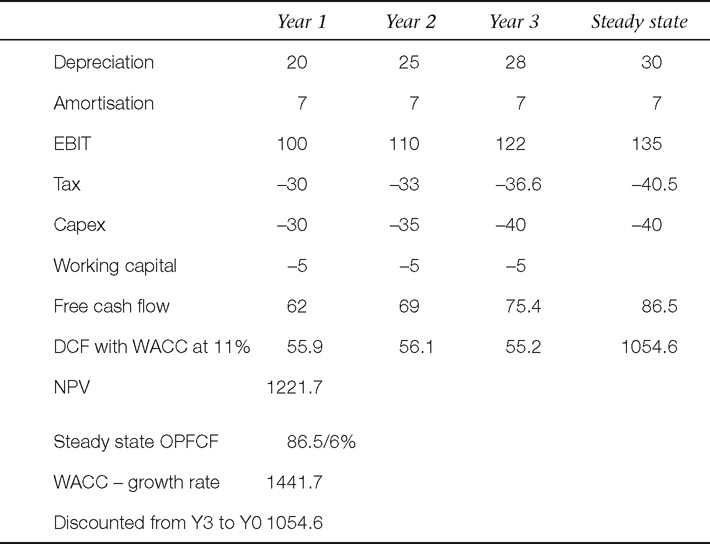
The DCF approach yields a net present value of £1221.7 million. The company will have debt of £300 million. This implies an equity value of:

However, if we feel that the broker is being too optimistic about:

• the steady state growth assumption of 5 per cent
• the level of risks involved

we can input our own assumptions. Let’s see what happens if the cost of capital rises to 13 per cent and the steady state growth rate falls to 3 per cent (Table 7.4).

Table 7.4 A rise in the cost of capital

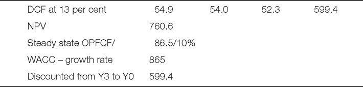
The 2 percentage point increase in the cost of capital and the 2 percentage point reduction in the steady state growth rate leads to an almost 40 per cent fall in the DCF to £760.6 million.

With debt fixed at £300 million the equity value would be:

This represents a fall in the equity value of 50 per cent. So a ‘tweaking’ of assumptions leads to a 50 per cent reduction in the value of the shares. The big impact is on the terminal value calculation, with the reduction in the growth rate and the higher cost of capital reducing the terminal value from £1054.6 million to £599.4 million. Instead of dividing the operating free cash flow by 6 per cent (11 per cent – 5 per cent) we are dividing by 10 per cent (13 per cent – 3 per cent). Therefore it can be seen how incredibly sensitive the company’s value is to relatively minor adjustments to changes in the assumptions. (It should be noted that this example is illustrative only, as in most DCF projections the initial growth phase would stretch out to Years 7–10.)

With this approach we can examine what has happened to the valuation of the high-tech growth stocks. Having disappointed expectations, growth forecasts have been reduced dramatically as it has become clear that they were susceptible to trends in the broader economy and in particular falling capital expenditure. Whether these areas of the market offer real growth is now increasingly questioned.

Effectively both the period and the extent of super-normal growth have been reduced, with devastating consequences for the DCF. Similarly, the extent of the growth at the terminal value stage has been revised down substantially. The development of operating profits and hence cash flow has therefore been downgraded dramatically.

The rising cost of capital as well as the downgrading of cash flow forecasts has also exerted pressure on valuations. The greater risks and higher volatility that have become increasingly apparent translate into a much higher cost of capital. The whole market has seen the equity risk premium rise, increasing that component of the cost of capital.

The substantial downgrades, as the impact of operational gearing became apparent, highlighted the volatility and risks at the individual stock level. In addition, the companies’ financial position deteriorated dramatically, with higher debt levels resulting from:

• debt taken on to fund deals that did not deliver hoped-for returns
• debt taken on for massive investment programmes
• the reduced profit forecasts and lower margins producing weaker cash flow and higher debt.

This combination of higher operational volatility and higher debt has led to the company’s beta increasing significantly.

A combination of these can see the discount rate required rise rapidly. An increase of 2 percentage points in the equity risk premium (ERP) and the move of, say, 1.5 to 2 in the beta can see the cost of capital rise considerably. With the risk-free rate at 5.5 per cent, if the ERP was 4 per cent and rose to 6 per cent, the cost of equity would rise from 11.5 per cent to 16.5 per cent. This would seriously damage the DCF valuation, as the examples illustrate.

• Forecast period of super-normal growth and returns? As discussed earlier, one of the key components in the DCF calculation is forecasting out to the terminal growth phase. This early period tends to be the period of ‘super-normal’ or higher growth. Again, the difficulty is forecasting both the level of this growth and how long this phase will last. With a growth industry a lot of capital may be attracted which depresses pricing below forecast levels. In addition, maturity can happen very quickly and the industry settles down into a more mature phase much earlier than anticipated. Mobile telephony is an industry which has seen explosive growth but has arguably become mature sooner than anticipated. With massive investment in new technology (3G), the low growth level damages the DCF model considerably. Much debate is taking place over what will be the key driver that will enable superior growth rates to be re-established.
• Complexity of calculation. For private investors in particular, the complexity of both doing the forecasts of operating cash flow and arriving at the cost of capital makes this approach to valuation rather esoteric. Finding the beta and the cost of debt can be awkward. Even if you do not intend to use this rather complex method, it is nonetheless important to be aware of its strengths and weaknesses to enable you to spot flaws in research that might be championing a share because of its attractiveness on DCF grounds and to help you approach it with a healthy dose of scepticism.

Summary

Given that cash is the ultimate driver of value, any asset is in effect worth the discounted value of its future cash flow. The value is derived from making long-term forecasts of a company’s cash flow and then ‘discounting’ these cash flows back into what that cash is worth today. Discounted cash flow is an ‘absolute’ measure of a company’s valuation and is sometimes referred to as net present value or intrinsic value. The discount rate used is the cost of capital which in theory reflects the risks attached to the company. That this risk is explicitly used in arriving at a valuation is clearly welcome.

To do a DCF effectively we need to forecast the price, volume and costs for the company long term and make assumptions about the capital expenditures and working capital requirements of the business. However, in an environment where forecasting the next quarter is challenging enough, using a method which relies on forecasting the next 10 to 20 years has many potential problems.

Having said that, while clearly challenging, having a sense of what the DCF generates as the value of the business is a useful exercise. We can feed in a variety of scenarios of prices and volumes (as well as other variables) to establish a feasible range for the valuation of the business. Alternatively, we can look at the stock market value of the business and then see what assumptions are being made about future operating profits and capital expenditures to arrive at that valuation. If you think these are too cautious you can see whether your assumptions led to a higher intrinsic value and buy the shares.

DCF is often viewed sceptically by some fund managers and analysts as the forecasts are so subjective and prone to revision. In addition, very ambitious/overoptimistic assumptions may be fed into the model to make the shares look attractive. This is often done during IPOs and was very much a feature of the floatations (and valuation of other businesses) during the dot-com boom. The valuations would be manipulated considerably by raising long-term growth forecasts or reducing the cost of capital – as we have seen, by making some very modest adjustments to our assumptions the equity value can be quickly halved or doubled.

Value investors will often look at out-of-favour and undervalued stocks and by doing a conservative DCF (or using a range of feasible assumptions) will see where the intrinsic value may lie. They can then assess whether the shares are worth buying on fundamentals despite the negative sentiment.