15 Maximizing High-Potential Accounts
The primary purpose of this chapter is to illustrate two common mistakes in sales development. They are:
1. Selling for volume rather than for profit.
2. Directing equal marketing pressure at all possible customers rather than concentrating on those with the highest potential.
To illustrate what I mean by this, I have put together four separate sales plans for the hypothetical Swing Corporation.
The Swing Corporation manufactures and markets an audio package for the elaborate-packaging market. Three models are offered: circuits, tubes, and valves. The sales plans are for the Northeast region, which represents approximately 10 percent of the corporation’s national market. The four sales plans are titled:
1. Forecasting by Sales Volume by Customer
2. Forecasting by Net Profit by Customer
3. Forecasting by Net Profit by Customer by Product/Service
4. Forecasting by Maximizing High-Potential Accounts
Forecasting by sales volume (Plan 1) is still the most prevalent means of determining sales for the following year. However, the problem is that sales volume by itself is meaningless. What good is it if you sell a million units and lose on each one? Forecasting by net profit by customer (Plan 2) is superior to Plan 1, but if you’re selling more than one product or service to the customer, you don’t know which ones are the winners and which ones are the losers. Therefore, forecasting by net profit by customer by product/service (Plan 3) is more effective than either Plan 1 or Plan 2. As you will see later in this chapter, when Plan 3 was used, it was determined that one of the three models (valves) was a money loser.
Forecasting by maximizing high-potential accounts (Plan 4) is based on the premise that you need to spend no more time or money on obtaining a 30 percent share of a 100-unit potential customer, which equates to 30 units, than on obtaining a 30 percent share of a 10-unit potential customer, which equates to only 3 units. Consequently, marketing efforts should be concentrated on those customers with the highest potential. Applying this principle to the hypothetical case history, total sales are decreased 8 percent, but net profit increases 273 percent.
Forecasting by Sales Volume by Customer (Sales Plan 1)
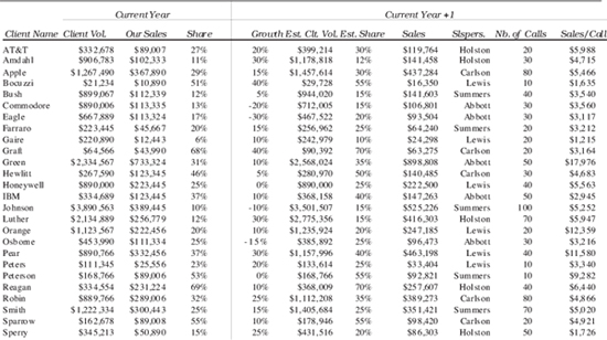
Figure 15–1 illustrates forecasting by sales volume by customer. Column 1 contains the names of the customers. Column 2 is an estimate of the client’s total purchases, from all suppliers, in the market segments in which the company competes. The third column shows the company’s sales to each of its clients. The data from columns 2 and 3 permit you to calculate your share of market by customer. For example, it is estimated that AT&T will buy $332,678 worth of elaborate-packaging products, and Swing Corporation’s share of those total purchases is estimated at $89,007, or 27 percent. The advantage of estimating your current share of market by client or account is that it permits you to forecast on the basis of share rather than sales. As mentioned, you can increase your sales and at the same time lose share. This situation could become a severe problem for you in the years ahead.
The fifth column in Figure 15–1 is an estimate of the growth in total purchases by customer for the next year. This growth rate can be applied to the current year client volume to obtain estimated client volume for the new year. Forecasting should then be based on your strategic choice of share increase, share maintenance, or share decrease. For example, the current estimated share for AT&T is 27 percent, and Swing wants to increase that share to 30 percent for the next year. Multiplying the estimated share by estimated client volume would then give you your sales forecast for the new period. In this case it’s $119,764.
The next column contains the name of the salesperson as well as his or her estimate on the number of sales calls that will be needed for the new year. This information can then be used to calculate the estimated sales volume by sales call. For example, Holston estimates that he will need twenty sales calls on AT&T for the new year, and the sales forecast is $119,764. This equates to a sales volume of $5,988 for each of the twenty sales calls.
At the bottom of Figure 15–1 is a summary of the estimated sales activity for each of the five salespeople for the new year. You will notice that, given these data, Summers, if he hits his forecast, will be the most effective salesperson. His total sales are projected at $1,534,868, and average sales per call are expected to be $6,382.
Figure 15–1 Forecasting by volume by customer—Plan 1.
However, this type of analysis can be very misleading if your company sells products/services with different margins. In these cases, the people who sell the most normally are not the ones who contribute the largest amount to profit. Why? Because they are selling the products/services that are the easiest to sell—and those usually have the lowest margins. Therefore, if these companies are rewarding their salespeople on the basis of volume, most likely they are rewarding the wrong people. Sales Plan 2 illustrates this fact.
Forecasting by Net Profit by Customer (Plan 2)
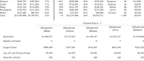
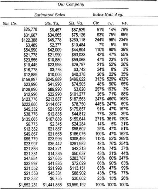
Sales Plan 2 is illustrated in three figures: Figure 15–2, which shows the estimated sales by product category; Figure 15–3, which calculates the margins by category and gross profit; and Figure 15–3a, which looks at expenses and profit per client per sales call.
If you are selling more than one product/service and they offer different margins, then the first step in forecasting net profit is to break out estimated sales for each. For example, we know from Sales Plan 1 (Figure 15–1) that total estimated purchases by AT&T are $119,764. In Figure 15–2, total estimated purchases are subdivided by model. It is estimated that AT&T will purchase $25,778 of the circuit model, $6,457 of the tubes model, and $87,529 of the valves model. Figure 15–2 also shows the percentage of client purchases by model type. Twenty-two percent of AT&T purchases will be for circuits, 5 percent for tubes, and 73 percent for valves. These percentage figures will be used later in Sales Plan 4 to determine company development.
In Figure 15–3, the first column contains the name of the client and columns two, three, and four list the gross profit by model. The margins are at the top of the column: circuits have a 17.07 percent margin; tubes, 10.59 percent; and valves, 4.15 percent. These margins are from the previous year. The fifth column contains the sum of columns two, three, and four, or total gross profit.
Figure 15–2 Sales by product category—Plan 2.
Moving on to Figure 15–3a, we see that the first three columns allocate the expenses per client. The first of these expense columns is for sales calls. Each sales call has been arbitrarily budgeted at $204.00. As we saw in Figure 15–1, Holston, the salesperson for AT&T, estimated that he would need twenty sales calls for the new year, or $4,080, so this is the amount listed underneath sales calls for AT&T in the first column. Other marketing costs and G&A have been allocated on the basis of last year’s expenditures as a percentage of sales.
Figure 15–3 Margin and gross profit—Plan 2.
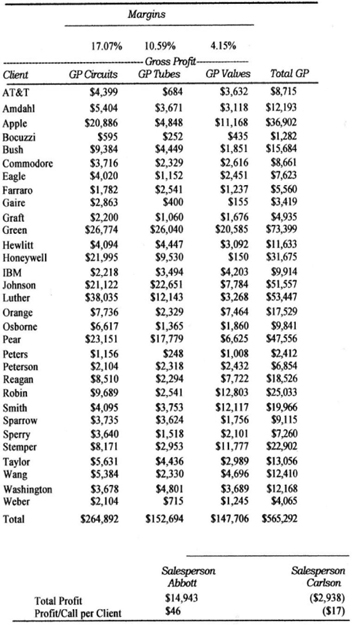
Figure 15–3a Expenses per client and total profit per sales call—Plan 2.
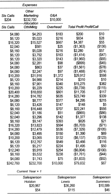
AT&T’s estimated total purchases of $119,764 (which also comes from Figure 15–1) are 1.8 percent of total estimated sales of $6,553,311. Multiplying 1.8 percent by total other marketing costs of $232,700 gives $4,253. This is the amount that is listed underneath other marketing for AT&T. The next column charges G&A; the same method is used for this as for other marketing costs. Now that expenses have been allocated by client, they can be subtracted from total gross profit to arrive at net profit by customer. The net profit shown for AT&T is $200.
When you know the total estimated profit by client or customer, you can calculate the estimated profit per sales call. This is shown in the last column of Figure 15–3a and a summary appears across the bottom of Figures 15–3 and 15–3a. You will notice that although Summers was projected to be number one in volume, he is not number one in either total profit or profit per sales call. Holston and Lewis are projected to deliver a higher total profit than Summers, with Summers and Abbott tied for number two in profit per sales call.
You will also notice in Figure 15–3a that several of the clients are showing a negative for total profit. Once again, if you analyze only volume, you cannot determine whether or not you are losing money servicing some customers. (This example uses clients or companies, but the same is true if your customer base is divided by markets.) Sales Plan 2 reveals that some clients are unprofitable, but it does not tell you which products/services sold to each customer or market are the losers. For example, client Eagle, which is the seventh client from the top, accounts for $7,623 in total gross profit, but shows a –$1,960 in total profit. Quite possibly, one or more of the models are profitable. The question is which ones. This question is addressed in Sales Plan 3.
Forecasting by Net Profit by Customer by Product/Service (Plan 3)
Sales Plan 3 is similar to Plan 2 except that in Plan 3 expenses have been allocated to each individual product. This cost allocation is based on percentage of sales. These calculations are shown at the top of Figure 15–4.
Sales costs have not been previously allocated by product categories, so the total sales calls budget for the Northeast region as shown in Figure 15–3a ($242,760) has been allocated to each product at the same percentage (3.7 percent). This percent is arrived at by dividing the total sales budget by total sales ($6,553,311, as shown in Figure 15–1). G&A has been handled the same way. However, other marketing expenditures have been previously budgeted by product category, so last year’s percent allocation has been used.
Let’s use AT&T again for an example. Figure 15–2 contains sales estimates by product or model category (circuits, tubes, and valves). The sales estimate on circuits for AT&T is $25,778. To obtain the net profit on circuits sold through AT&T, you would multiply the $25,778 estimated sales volume by the gross margin of 17.06 percent. This would give you a gross profit of $4,399. This amount appears in the second column in Figure 15–4, in the row for AT&T. To obtain the net profit on circuits from AT&T, you would multiply the sales volume estimate of $25,778 by the cost allocation (based on a percentage of sales) for sales, other marketing, and overhead expenses. By multiplying the total cost allocation of 7.44 percent by the total estimated volume of $25,778 and subtracting this total expense item from gross profit, you will receive net profit in the amount of $2,482. This amount appears in the fifth column in Figure 15–4 underneath net profit on circuits.
Figure 15–4 Net profit by product—Plan 3.
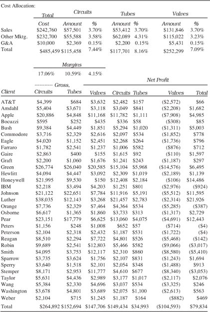
If you look across the bottom line in Figure 15–4 at the totals, you will notice that the net profit on circuits is projected at $149,434; on tubes, $34,993; and on valves a loss of $104,593. In other words, as the company is now operating, being in the valve business is costing it over $100,000 a year. As previously mentioned, the sad part about a situation like this is that most companies do not realize that one or more products/services are literally dragging down their total profit—and they are not aware of it because they do not calculate net profit by individual products or services.
Now, you may be thinking to yourself that it would be a great idea to break out expenses by product or service category, but you conclude that you cannot physically calculate these numbers. I would reply that you are copping out. Regardless of the product/service, it is not that difficult to allocate the costs or expenditures, especially when you take into consideration the 20/80 rule of thumb—that is, 20 percent of the activity, whether it be manufacturing or administration, probably accounts for over 80 percent of the total cost or expenditure. Therefore, just measure or monitor the manpower, machines, and so on that are used most extensively or are the most expensive and you will quickly get the figures you need.
Forecasting by Maximizing High-Potential Accounts (Plan 4)
As mentioned at the beginning of this chapter, the premise behind Plan 4 is that it should be no harder, and cost you no more, to go after the high-potential markets or customers than to pursue the average or below-average customer. IBM has been going to the data processing people in the large companies and saying, “I hear you have a problem.” The data processing people say, “We sure do. We’ve lost control, because all our employees are going out into the marketplace and selecting their own PCs. In addition, when we have to tie all these PCs together or network them, we really are going to have a severe problem.” What is the IBM salesperson’s reply? Simple: She pulls out a contract for 200 IBM PCs and shows it to the data processing people. The IBM salesperson says that if they sign the contract, they will be back in control. They can pass out the IBM PCs to the employees, and when they have to network the system, it will be a piece of cake, because all the machines will be IBM. What are the data processing people going to do? Sign the contract, obviously. Meanwhile, the competitors’ salespeople are spending an equal amount of time trying to sell one or two of their computers.
Our illustration of forecasting by maximizing high-potential ac counts will be divided into five parts. They are:
1. Estimated sales potential and company development (Figure 15–5 and 15–5a)
2. Number of share points per marketing unit and cost per marketing unit (Figure 15–6)
3. Forecasting by maximizing high-potential accounts—circuits (Figures 15–7 and 15–8)
4. Forecasting by maximizing high-potential accounts—tubes (Figures 15–9 and 15–10)
5. Forecasting by maximizing high-potential accounts—valves (Figures 15–11 and 15–12)
Figure 15–5 contains estimated client total purchases by product category. Figure 15–5a indexes clients’ purchases against the national average. For example, AT&T’s total purchases for circuits for the new year are estimated at $122,776. This is only 57 percent of the national average. The national average (in this case, the Northeast region) is calculated by dividing the number of clients (31) into total estimated purchases ($6,682,266). This gives you the national average of $215,557. AT&T’s total purchases are 43 percent below this national average. AT&T is also low in potential on tube purchases, with its total estimated purchases equaling only 18 percent of the national average. Its valve purchases are only 60 percent of the national average. Conversely, the second client listed, Amdahl, would be considered an extremely high-potential customer, because the estimated circuit volume is more than twice the national average, volume for tubes is 14 percent above the national average, and volume for valves, 27 percent over.
The third client, Apple, is similar to Amdahl, with total estimated purchases for each of the three product categories being considerably above the national average. By contrast, the fourth client, Bocuzzi, offers such low potential that it is literally impossible to handle this account at a profit. This does not mean that you should completely disregard customers that account for very small volume, especially if there is a possibility that they will increase their purchases in the future. The point is that you should not be servicing an account like Bocuzzi the same way you are servicing accounts such as Amdahl and Apple.
On the right-hand side of Figure 15–5a is estimated company sales by product category. These sales data have been picked up from Figure 15–2. As was done with client potential, company sales have also been indexed versus the national average. For example, estimated circuit sales to AT&T are approximately half of the national average for circuits, tube sales are estimated to be only 14 percent, and valve sales, 76 percent. Company-estimated sales to Apple illustrate the opposite extreme. Both estimated circuit and valve sales are more than twice the national average.
Figures 15–5 Estimated sales potential—Plan 4.
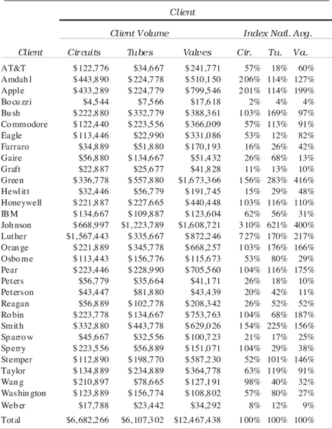
Figure 15–5a Company development—Plan 4
This indexing of estimated sales versus the national average is referred to as brand/service or company development. Ideally, what you should be trying to accomplish through your marketing efforts is to obtain above-national-average development in markets or companies that have above-average potential. That is another way of saying that your objective should be to obtain a share in high-potential markets or accounts that is equal to or greater than your share in lower-potential markets or accounts.
The share objective for the Northeast region is 26 percent, as stated in Figure 15–1. This is a very good way to set a reasonable goal: your share of a particular high-potential client should equal your share of that market. Applying this share objective against AT&T’s total estimated purchase of circuits in the amount of $122,776 yields $31,921. This approximates the sales estimate for AT&T, as shown in Figure 15–5. However, if we apply the 26 percent share goal against the total estimated purchases of circuits by Amdahl, this comes to $115,411. The company’s current sales estimate is only $31,667. The question is, is it really that much more difficult to obtain a 26 percent share of the Amdahl business than to get 26 percent of the AT&T business? Not really—if you point these discrepancies out to your marketing people and then reward them on the basis of profit rather than volume.
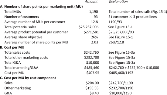
Now that client potential as well as company development has been determined, the next question is, how much marketing pressure should be applied against each client, and what will be the cost? These questions are answered in Figure 15–6, which contains the second step we must take to maximize our high-potential customers.
The first part of Figure 15–6, Section A, shows how we determine the number of share points that should be obtained per marketing unit. A marketing unit, referred to in abbreviated form as MU, is an arbitrary amount of marketing weight. In this case history, the total number of estimated sales calls listed in Figure 15–1 has been used as the number for the total number of marketing units available. This figure is 1,190, as indicated on the first line under Section A in Figure 15–6. This number could just as well have been 1,000, 10,000, or 500. It is an arbitrary figure that you use to:
Figure 15–6 Marketing units: share points, cost, and cost by cost component.
1. Determine the number of units of marketing pressure that will be applied against each customer, market, or client.
2. Allocate marketing and other appropriate expenditures for each market or customer.
The next item is the number of customers. Here 93 has been used. The explanation is that there are thirty-one customers and three product lines; 3 times 31 equals 93. (The assumption is that each of the customers purchases each of the product lines.) This permits calculation of the average number of market units per customer, dividing the total number of marketing units available (1,190) by the number of customers (93) to reach 12.8, the weight of our MU.
The next line states total potential sales, and the answer is $25,257,006. This comes from Figure 15–1. Then comes another calculation, average product potential per customer. The answer is $271,581, this being the result of dividing $25,257,006 by 93. The average share objective follows; this is 26 percent, again lifted from Figure 15–1. With all the above information, you can now calculate the average number of share points that should be obtained per marketing unit, which is 2.03. This is simply 26 percent divided by 12.8.
To state this in another way, we have now determined the amount of marketing pressure that should be applied per share point in high-potential accounts. If the share objective is 26 percent, that will mean approximately thirteen sales calls (26 percent divided by 2.03) and thirteen units of other types of marketing effort that are being used. If the share objective is 10 percent, it will mean approximately five sales calls. And so on.
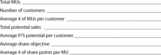
Here’s a worksheet for you to calculate the number of share points per marketing unit for your company. It’s really pretty straightforward if you go step by step. You can make a photocopy of this, or print out a copy from the Worksheets folder that you downloaded to your computer.
Worksheet 15–1 Number of share points per marketing unit
Now that the number of share points per marketing unit has been determined, the next step is to calculate the marketing cost for each marketing unit. This is calculated under Section B in Figure 15–6. According to Figure 15–3a, total sales costs are estimated at $242,760, other marketing expenditures at $232,700, and G&A costs at $10,000. The sum of these figures results in a total marketing/G&A cost of $485,460, which is divided by number of MUs (1,190), to give a cost per marketing unit of $407.95. You will note that G&A costs have been included along with marketing. The reason for this is that it permits a calculation of net profit.
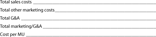
Use Worksheet 15–2 to calculate costs per marketing unit for your company.
Worksheet 15–2 Cost per marketing unit
Section C of Figure 15–6 is a breakout of the cost of a marketing unit into sales, other marketing expenditures, and G&A. Worksheet 15–3 enables you to break out your cost per marketing unit by cost component.
Worksheet 15–3 Cost per marketing unit by cost component

The preceding calculations give us sufficient data to apply the principle maximizing high-potential accounts. This is illustrated in the next three tables, with Figure 15–7 covering circuits; Figure 15–8, tubes; and Figure 15–9, valves.
In Figure 15–7, the first column lists the various clients, but unlike in the previous tables, the clients have been rearranged on the basis of their potential purchases of circuits. This is a numerical sort in descending order of the national average index from Figure 15–5. You will notice that the client Luther (how did that happen?) is estimated to have the highest potential on circuits, with an index of 727 percent, or seven times the national average. The next client, Johnson, has an index of 310 percent, which is three times the national average. Amdahl has an index of 206 percent, and so on. Clients Luther through Honeywell, which have an above-average potential, are listed at the top of the table, and clients with an index below 100 percent, or lower than the national average, are listed in the lower half.
The reason for this division is that two separate strategies will be used—one for above-average-potential customers and another for below-average-potential customers. The strategy for high-potential ac counts is stated at the top of Figure 15–7, “Increase development to level of potential in high-potential accounts and allocate marketing and G&A expenses on basis of share objective.” The strategy for low-potential accounts is stated in Figure 15–8: “No increase in sales in low-potential accounts and no marketing units against ac counts where just one MU would generate a loss.” The meaning of these two strategies will become clearer as the rest of the table is discussed.
Starting at the top, we see in Figure 15–7 that the first client listed is Luther. The second column shows estimated total circuit purchases, with the index (that is, potential circuits) shown in the third column. The fourth and fifth columns are on company development, with column four being the index and column five being the volume. The data for both these columns are picked up from Figure 15–5a. The sixth column contains the revised development objectives; the figure is picked up from either column three or column four, whichever is larger. For example, the revised development for Luther is shown as 727 percent, and this equals the potential index in column three. In the case of Apple, which is the fourth client down, the development objective is 244 percent, which is picked up from column four because the current company development is greater than the potential. An alternative way of stating this strategy on new development objectives is that sales goals will be equal to the client potential or current company development, whichever one is higher.
Figure 15–7 Above average potential—circuits.
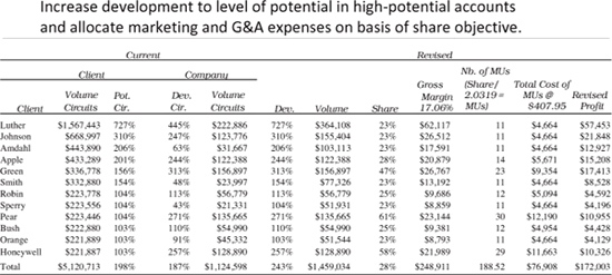
These new development objectives are used to calculate the revised sales volume, which is shown in column seven. The next column translates these volume figures into share, with the average share for high-potential accounts equaling 28 percent. The ninth column lists the gross margin. This figure minus the marketing-unit expenditure detailed in the next two columns results in the revised profit shown in the farthest column to the right.
Going back to the two columns between the gross margin and the revised profit, the one on the left details the number of marketing units to be used, and the one on the right states the total costs of the marketing units. For example, eleven marketing units will be used against Luther, because if you divide 2.03 into the 23 percent share objective, you will get 11. The total MU expenditure charged against Luther is eleven times the cost per unit (11 × $497.95).
All you have to do is look at the total revised profit for the high-potential clients on circuits alone, and you will realize what a dramatic effect this type of sales-development strategy can have on your bottom line. The total revised profit for both low- and high-potential clients, as shown in the very bottom row in the right-most column of Figure 15–8, is $175,891, which exceeds the total previous indicated profit for all three product categories against all thirty-one clients.
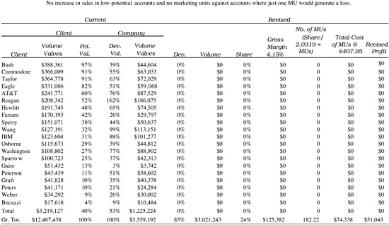
Figure 15–8 executes the strategy for low-potential clients, which, as stated above, is, “No increase in sales in low-potential accounts and no marketing units against accounts where just one MU would generate a loss.” For example, clients Wang through Commodore can still offer profitable business, but clients Eagle through Bocuzzi are impossible to service without incurring a loss, because the cost of a marketing unit exceeds the gross profit generated by the resulting share points. For example, one marketing unit (one sales call, and so on) on a national average comes out to approximately a two share. A two share of the client potential on client Eagle is $2,268 ($113,446 × 0.02). The gross margin on $2,268 at the rate of 17.06 percent equals $387. This is less than the cost of a marketing unit, which is $407. This is not to say that in the real world you should completely eliminate clients such as Eagle through Bocuzzi, but it should indicate to you that you have to handle this type of business with a different strategy—maybe just telemarketing, or just brochures.
You can’t solve a problem until you can spot it and only then develop new strategies. For example, Johns Hopkins University researchers were frustrated by the high school dropout rate. That was their problem. So they did research and found a high correlation between poor attendance of eight-graders and their subsequent dropout rate. Now the schools have special programs to help those with this profile.
Figures 15–9, 15–10, 15–11, and 15–12 are the same as Figures 15–7 and 15–8, except that they concern different product lines: tubes and valves. These exhibits illustrate that for these two products, no client below the national average in potential can be handled profitably. The reason is that these gross margins are much lower than for circuits.
Figure 15–8 Below average potential—circuits.
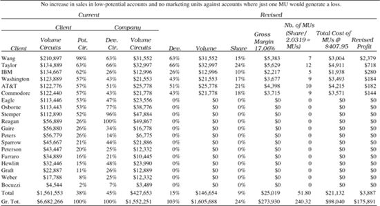
Figure 15–9 Above average potential—tubes.
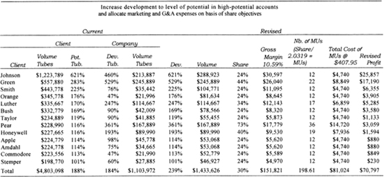
Figure 15–10 Below average potential—tubes.
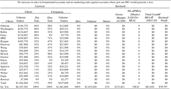
Figure 15–11 Above average potential—valves
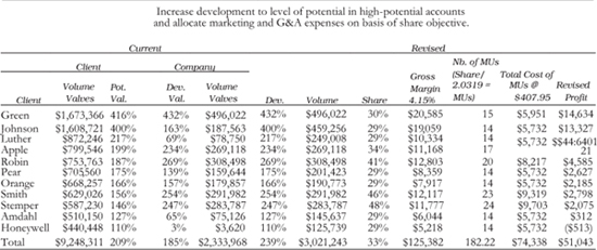
Figure 15–12 Below average potential—valves.
What Have We Learned?
Figure 15–13 is a summary of the four sales plans.
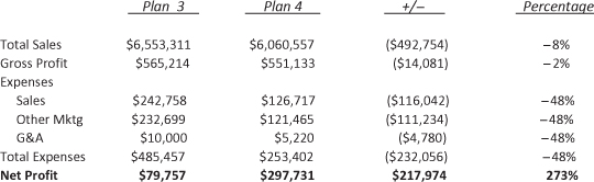
Figure 15–14 presents what is probably of greatest interest. It compares Plan 3 and Plan 4. It shows that total sales for Plan 4 are 8 percent lower than for Plan 3 and that gross profit is 2 percent lower. However, expenses for Plan 4 are 48 percent lower than for Plan 3, resulting in a net-profit increase of 273 percent for Plan 4 over Plan 3. The reason for the large decrease in expenditures is that the number of MUs has been cut from 1,190 to 621. This would require fewer sales personnel; the staff can be reduced through either transfers or attrition.
Figure 15–13 The four sales plans.
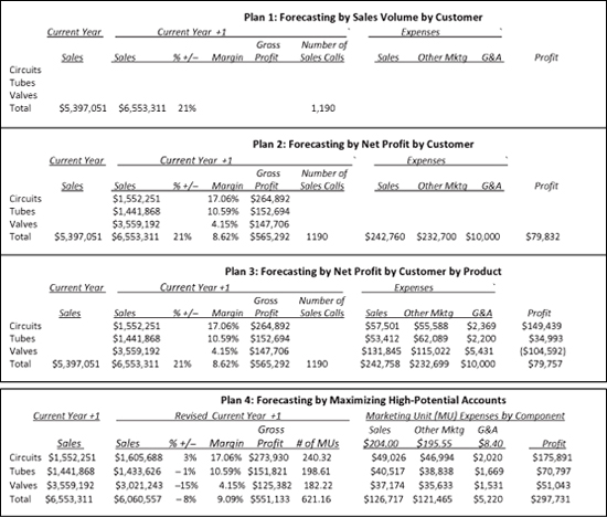
Figure 15–14 Plan 3 versus Plan 4.
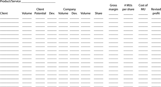
Worksheet 15–4, which ends this chapter, enables you to finish your own analysis of your client base. If you have already completed Worksheets 15–1, 15–2, and 15–3 to establish your MUs, then go ahead and fill out Worksheet 15–4 now. If you haven’t, go back and do them first. If you don’t know your clients’ sales potential, assign that task to your sales force. The rest of the data you should have in house.
Worksheet 15–4 Forecasting by maximizing high-potential accounts