
12 The Sales Plan: Pricing
In determining the price for their product/service, many companies just add up all their costs and arbitrarily add a certain amount for profit—and that becomes their selling price. The question is: Is this price giving them the maximum marginal income?
Apple, Inc. is doing very well right now financially. Of course, their iPhone is a big winner. But their Mac computer only has a 7.6 percent market share in the United States as of the second quarter of 2009, and only 3.36 percent worldwide. Dell has a 26.3 percent share and Hewlett-Packard has a 26 percent share. I believe many people would agree that the Mac has better graphics and an operating system superior to that of PCs, such as Dell and HP, which run Microsoft Windows. Then why is their market share so low? I believe it is because they are premium priced. If they dropped their price to match Dell and HP would their shares double or triple?
Conversely, Australia Chardonnay wine was a good seller here in the United States until recently. They kept dropping their price to the point that people began to think it was inferior and consequently, they started losing sales. These two tales are my way of saying that you may want to do some research to see if you have an optimum price.
The first two matrixes of the pricing model (CPRICING.xls) are shown in Figure 12–1. The first matrix establishes fixed costs. This pricing model case history is based on a proposal that includes a $10,000,000 plant (shown in Figure 12–5). In this hypothetical situation, we are depreciating the building over five years or $2,000,000 per year. Corporate fixed costs are estimated to be somewhere between $300,000 and $500,000, operational fixed costs between $8,200,000 and $9,500,000, and the cost for our own staff, which includes management and others who are not directly involved in production, at $3 million. This gives a total fixed cost estimated to be somewhere between $13,500,000 and $15,000,000 per year.
The second matrix on Figure 12–1 concerns the selection of the selling price. The variables are estimated variable costs (VC high versus VC low), selling price, and estimated sales at that price. In our example, the estimated high variable cost is $1,500 and the low variable cost $1,350. In contrast to fixed costs, variable costs vary relative to the number of units. If this company comes in at its estimated high variable cost of $1,500, that means that the cost of goods, labor, and other variable costs would be approximately $1,500 per unit. After the variables are inserted, the computer will determine the marginal income per unit as well as the total marginal income for both the high and low variable costs. What you are looking for here is the price that will give you the highest total marginal income, whether you have high or low VC. We see that the highest total marginal income ($15 million and $18 million, respectively) is generated when our sales price is $2,100.
If the item is priced at $800 per unit, estimated sales are projected at 120,000 units. However, if the company came in with its high variable cost, it would lose $700 per unit and if it came in with its low variable cost, it would lose $550 per unit. At the other extreme we see the high selling price of $2,800. Here the sales projection is 10,000 units. The marginal income per unit would be $1,300 if the company comes in with its high variable cost and $1,450 if they come in with their low variable cost. However, because the total unit sales are so low (10,000), this high price still does not give us our highest total marginal income. Total marginal income is the marginal income per unit (selling price minus variable cost) times estimated sales.
Figure 12–1 Pricing model: Establishing fixed costs and selection of selling price (CPRICING; range name: First Half).
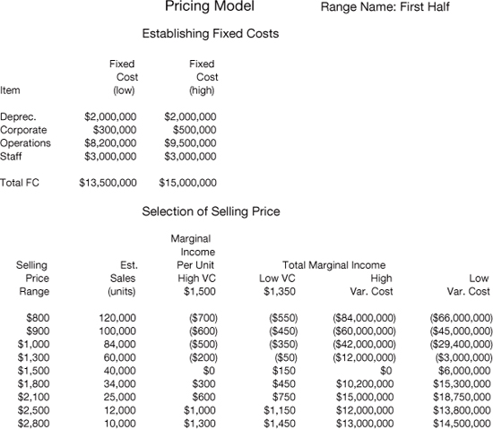
As we see in Figure 12–1, at a selling price of $2,100, the total marginal income is estimated to be between $15,000,000 and $18,750,000.
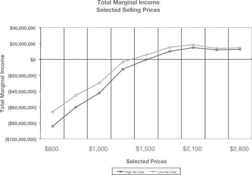
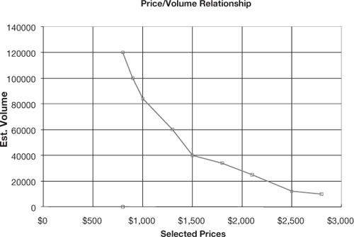
Figure 12–2 (Total Marginal Income) shows a chart from the Excel file (chart name: MARGINCOM) illustrating the total marginal income for both the high and low variable costs. Notice that each line chart peaks at $2,100. Figure 12–3 (Price/Volume Relationship) is an XY chart from the Excel file (chart name: PRICEVOL) depicting the relationship between the various prices and the estimated volume for each. This line should always be a relatively smooth curve, with the curve being close to the horizontal for products or services that are insensitive to price (for example, Scotch) and more vertical when they are price sensitive (for example, paper napkins, paper towels, etc.). It is clear from the slope of the curve that our hypothetical product is price sensitive.
Figure 12–2 Total marginal income (CPRICING; chart name: MARGINCOM).
The second half of the pricing model (range name: Second Half), as shown in Figure 12–4, determines the high and low marginal income on both a unit and a percentage basis. The two variables are the high and low sales price. In the previous section of the model, it was determined that the optimum sales price should be $2,100. That figure is inserted in the column marked high in the model. For the low price we have taken the price immediately below the highest price. The reason for this is that even if you price a product or service at $2,100, the trade is going to try and beat you down to get a lower price. After we have inserted our two variables, the computer model picks up the low variable cost against a high sales price to give us our maximum marginal income per unit of $750 or 36 percent. The other extreme or least favorable scenario would mean a $1,800 sales price with our high variable cost of $1,500, giving us a marginal income per unit of only $300, which is a mere 17 percent return.
Figure 12–3 Price/volume relationship (CPRICING; chart name: PRICEVOL).
Now that we have our high and low marginal income, we can determine our breakeven points, which is the second part of this figure. The column on the left is our most favorable scenario and the column to the far right is our least favorable scenario. For example, if we come in with our low fixed cost of $13,500,000 and our high marginal income of $750 per unit or 36 percent, then our breakeven point is only $37,800,000. However, if we come with our high fixed cost of $15,000,000 and our low marginal income of only $300 per unit or 17 percent, our breakeven point skyrockets all the way up to $90,000,000.
Figure 12–4 Pricing model: High/low marginal income, breakeven points, and net income (CPRICING; range name: Second Half).
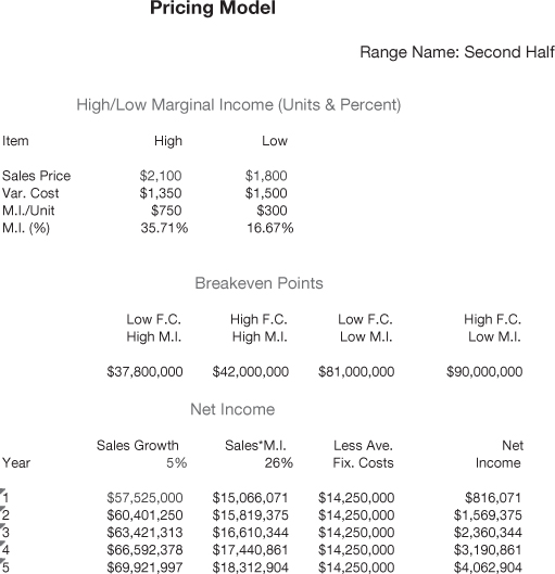
The third matrix on Figure 12–4 gives us our net income. The variables here are annual sales growth rate and first-year sales. First-year sales can either be the recommended sales price of $2,100 multiplied by estimated sales of 25,000 units, or, if you wanted to be conservative, it could be an average of the high and low selling price times the average for the estimated sales for each of these particular prices. For example, you could take the average between $2,100 and $1,800, which would be $1,950; and the average between the estimated sales for each price, 34,000 and 25,000, or 29,500. Multiplying $1,950 times 29,500 units would give you the first-year sales of $57,525,000. To determine the marginal income, the computer takes the average between the previously calculated high and low margins (36 percent and 17 percent) or 26 percent. Therefore, after subtracting the estimated average cost for labor, cost of goods, etc., marginal income for the first year will be $15,660,071. From this is subtracted average fixed cost of $14,250,000, resulting in a net income of $816,071. For years 2 through 5, the computer increases annual sales at the rate of 5 percent, which will provide an annual net income at the end of year 5 of $4,062,904.
The last part of our hypothetical pricing model, as shown in Figure 12–5, is discounted cash flow.
Actually, the most important factor or number in this entire model is a variable that you see underneath the discount factor in the far right-hand column. What the 17.4 percent means is that if all the preceding figures are correct, then you will be receiving a 17.4 percent return on your money after taxes. We’ll return to this figure in a moment. Going over to the left-hand side of this part of the model, the variable is the tax rate. What has been inserted is 46 percent. The computer then multiplies the net income from the preceding part of the model, giving us a net income after taxes of $440,679 for the first year. Then adding back in depreciation, you get a total cash flow at the end of the first year of $2,440,679. The cash outlay or the cost of the plant ($10,000,000) is shown underneath the initial cost column. For years 1 through 5, the total cash flow is $16,479,760. On a discount factor or net present value, this gives you a 17.4 percent return on your money.
Figure 12–5 Discounted cash flow (CPRICING; range name: DCF).
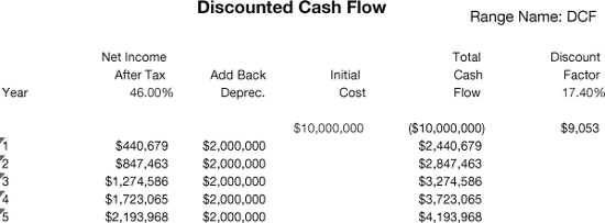
The net present value formula goes in the cell that currently contains $9,053. Then, after you have completed all parts of the model, you keep varying the percentage figure immediately under the column titled “discount factor” until the number two rows below becomes the closest to zero. For example, if you change the discount factor from 17.4 percent to 17.5 percent, the figure two rows below would become –16,046. If you change the discount factor to 17.3, it would become 34,251. Therefore, 17.4 percent is the correct discount factor or return on this company’s money. (We used this reasoning in calculating discounted cash flow when we were discussing the product/service plan, back in Chapter 6, remember?)
Obviously, a 17.4 percent return after taxes is very favorable. If management of this hypothetical company were in agreement with all of the previous figures in this model, then quite likely the company would go ahead with this proposal because it gives a very attractive return. If the return was only 5–10 percent after taxes, then most likely it would not be a viable project. The reason is that it’s possible to buy municipal bonds at a 10–12 percent return with no taxes and little risk.
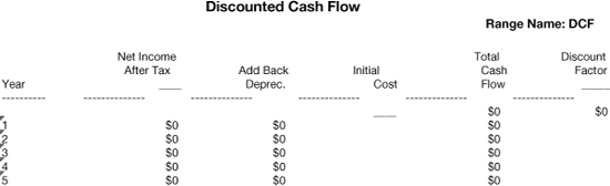
Figures 12-6, 12-7, and 12-8 show the two ranges in the electronic file PRICING.xls, which you can use for your own data. Remember, you only fill in the blue areas and zeros. The black zeros are formulas.
Figure 12–6 Your pricing model: Establishing fixed costs and selection of selling price (PRICING; range name: First Half).
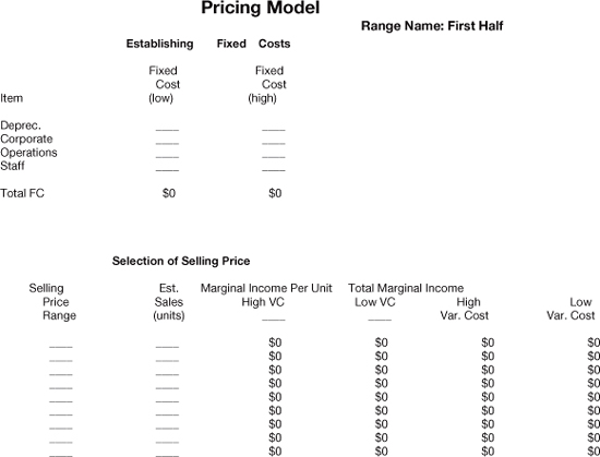
Figure 12–7 Your pricing model: High/low marginal income, breakeven points, and net income (PRICING; range name: Second Half).
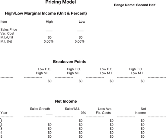
Figure 12–8 Your discounted cash flow (PRICING; range name: DCF).
The reason the discounted cash flow factor is so helpful is that it enables you to compare the rate of return on your money for various projects or ventures. This particular project would return 17.4 percent after taxes. This can be compared with the current return on the stock market, money funds, bonds, etc., as well as various other projects. In addition to the rate of return, the other factor to be examined is risk. For example, if a company was able to obtain 10 percent return after taxes on a venture that had a very low risk such as municipal bonds, this would probably be a better investment than introducing a new product or service that only promised a 12 percent return. In this particular case, there is only a two-point spread between something that has very little risk versus a product or service introduction, which of course always involves considerable risk.
This is the first of two chapters on the Sales Plan. The objectives and strategies worksheet for this segment will be at the end of the next chapter.