7. Text Generation and Summarization

Overview

This chapter begins with the concept of text generation using Markov chains, before moving on to two types of text summarization—namely, abstractive and extractive summarization. You will then explore the TextRank algorithm and use it with different datasets. By the end of this chapter, you will understand the applications and challenges of text generation and summarization using Natural Language Processing (NLP) approaches.

Introduction

The ability to express thoughts in words (sentence generation), the ability to replace a piece of text with different but equivalent text (paraphrasing), and the ability to find the most important parts of a piece of text (summarization) are all key elements of using language. Although sentence generation, paraphrasing, and summarization are challenging tasks in NLP, there have been great strides recently that have made them considerably more accessible. In this chapter, we explore them in detail and see how we can implement them in Python.

Generating Text with Markov Chains

An idea is expressed using the words of a language. As ideas are not tangible, it is useful to look at text generation in order to gauge whether a machine can think on its own. The utility of text generation is currently limited to an auto-complete functionality, besides a few negative use cases that we will discuss later in this section. Text can be generated in many different ways, which we will explore using Markov chains. Whether this generated text can correspond to a coherent line of thought is something that we will address later in this section.

Markov Chains

A state space defines all possible states that can exist. A Markov chain consists of a state space and a specific type of successor function. For example, in the case of the simplified state space to describe the weather, the states could be Sunny, Cloudy, or Rainy. The successor function describes how a system in its current state can move to a different state or even continue in the same state. To better understand this, consider the following diagram:

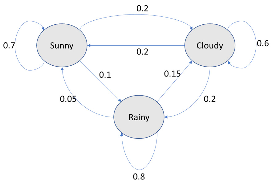
Figure 7.1: Markov chain for weather

The successor function of a Markov chain is a random selection of a successor state based on probabilities. For instance, consider that the initial state is randomly selected as Rainy. The next state could be Rainy (there is a 0.8 probability that the state stays Rainy). Then, the next state could be Sunny (there is a 0.05 probability associated with this transition). It could be Rainy again, and then it could be Cloudy, and so on. Our sequence of states is Rainy-Rainy-Sunny-Rainy-Cloudy. For each state, the successor state is found by a random selection; this is called a random walk on the Markov chain.

Similarly, if we have a state space in which the states correspond to a vocabulary, then a random walk on such a Markov chain will generate text. Now, the vocabulary could have around 20,000 words. In this case, the Markov chain will have 20,000 states. The probabilities in this case will correspond to the likelihood of a word succeeding a given word. We can begin with any state randomly drawn from among the words that could be used for the first word of a sentence, for example, common words such as "the, " "a, " "I, " "he, " "she, " "if, " "this, " "why, " and "where". We then find its successor state in a random way, followed by the next successor state found in a random way, and continue in the same manner until we have generated a sequence of words of the required length. In the next section, we will do an exercise related to Markov chains to get a better understanding of them.

Exercise 7.01: Text Generation Using a Random Walk over a Markov Chain

In this exercise, we will generate text with the help of Markov chains. We will use Robert Frost's collection of poems, North of Boston, available from Project Gutenberg, to specify the successor state(s) for each state using a dictionary. We'll use a list to specify the successor state(s) for any state so that the number of times a successor state occurs in that list is directly proportional to the probability of transitioning to that successor state.

Then, we will generate 10 phrases with three words in addition to an initial word, and then generate another 10 phrases with four words in addition to an initial word. The initial state or initial word will be randomly selected from among these words: "the," "a," "I," "he," "she," "if," "this," "why," and "where." Note that since we are generating text using a random walk over a Markov chain, in general, the output you get will be different from the output shown in this exercise. Each different output corresponds to new text generation.

Note

You can find the text file that's been used for this exercise at https://packt.live/2DiGAE3.

Follow these steps to complete this exercise:

1. Open a Jupyter notebook.
2. Insert a new cell and add the following code to import the necessary libraries and read the dataset:

   import re

   import random

   OPEN_DATA_URL = '../data/robertfrost/pg3026.txt'

   f=open(OPEN_DATA_URL,'r',encoding='utf-8')

   text=f.read()

   f.close()

3. Insert a new cell and add the following code to preprocess the text using regular expressions:

   HANDLE = '@w+ '

   LINK = 'https?://t.co/w+'

   SPECIAL_CHARS = '<|<|&|#'

   PARA=' +'

   def clean(text):

       #text = re.sub(HANDLE, ' ', text)

       text = re.sub(LINK, ' ', text)

       text = re.sub(SPECIAL_CHARS, ' ', text)

       text = re.sub(PARA, ' ', text)

       return text

   text = clean(text)

4. Split the corpus into a list of words. Show the number of words in the corpus:

   corpus=text.split()

   corpus_length=len(corpus)

   corpus_length

   The preceding code generates the following output:

   19985

5. Insert a new cell and add the following code to define the successor states for each state. Use a dictionary for this:

   succ_func={}

   corpus_counter=0

   for token in corpus:

       corpus_counter=corpus_counter+1

       if corpus_counter<corpus_length:

           if token not in succ_func.keys():

               succ_func[token]=[corpus[corpus_counter]]

           else:

               succ_func[token].append(corpus[corpus_counter])

   succ_func

   The preceding code generates an output as follows. Note that we're only displaying a part of the output here.

   

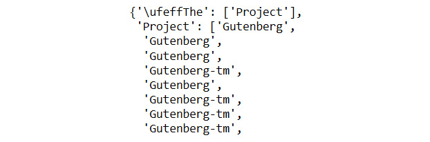
   Figure 7.2: Dictionary of successor states

   We find that "he" is shown as a successor of "who" more than once. This is because this occurs more than once in the dataset. In effect, the number of times the successors occur in the list is proportional to their respective probabilities. Though it is not the only method, this is a convenient way to represent the successor function.

6. Define the list of initial states. Then, define a function to select a random initial state from these and concatenate it with successor states. These successor states are randomly selected from the list containing successor states for a specific current state. Add the following code to do this:

   initial_states=['The','A','I','He','She','If',

                   'This','Why','Where']

   def generate_words(k=5):

       initial_state=random.choice(initial_states)

       current_state=initial_state

       text=current_state+' '

       for i in range(k):

           succ_state=random.choice(succ_func[current_state])

           text=text+succ_state+' '

           current_state=succ_state

       print(text.split('.')[0])

7. Insert a new cell and add the following code to generate text containing 10 phrases of four words (including the initial word) and 10 phrases of five words (including the initial word):

   for k in range(3,5):

       for j in range(10):

           generate_words(k)

   The preceding code generates the following output:

   

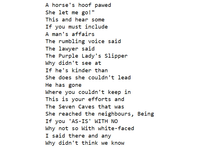
Figure 7.3: Phrases generated, consisting of four and five words

Note

To access the source code for this specific section, please refer to https://packt.live/313fiJY.

You can also run this example online at https://packt.live/33ilO2l.

It's quite interesting that we are able to generate text using a random walk over a Markov chain. If we look more closely, we will see that only a few of the phrases make sense. Broadly speaking, we are generating text that has an element of Robert Frost's style. However, it can hardly be said to correspond to a thought of any kind.

The practical utility of generating text using a Markov chain is somewhat limited to generating spam (spam generators could use a Markov chain) and generating something that is a little amusing. Nevertheless, this exercise demonstrates the surprising results we can get by using a simple approach in which nothing about the structure of a language is explicitly taught to the machine.

In general, auto-complete is one positive use case and arguably the sole positive use case for text generation given that other use cases (besides spam) tend to include the generation of misinformation.

Paraphrasing involves replacing some text with different text that has the same meaning. Now, intuitively, a machine will be able to tell whether one piece of text is a paraphrase of another, but only if that machine understands the meaning. So, one way of checking whether a machine understands the meaning of a piece of text is to check if it can tell if another different piece of text is a paraphrase of that first text.

Benchmark datasets provide a standard touchstone for evaluating approaches to solve a problem. The approaches are typically ranked in a publicly available leaderboard. Even in the case of such benchmark datasets, as of February 21, 2020, the SuperGLUE leaderboard (https://super.gluebenchmark.com/leaderboard) sets human baselines at the top when considered across a variety of tasks. This means that humans are superior at paraphrasing than the most sophisticated approaches even on the specified datasets. Paraphrasing is even tougher outside of benchmark datasets because it is tougher to teach models in a more general way so that the model is as effective for other datasets. Thus, compared to machines, humans can paraphrase even better on other datasets than machines can. In short, paraphrasing using NLP is challenging and is currently of limited practical utility to the practitioner. In the next section, we will learn about summarization.

Text Summarization

Automated text summarization is the process of using NLP tools to produce concise versions of text that preserve the key information present in the original content. Good summaries can communicate the content with less text by retaining the key information while filtering out other information and noise (or useless text, if any). A shorter text may often take less time to read, and thus summarization facilitates more efficient use of time.

The type of summarization that we are typically taught in school is abstractive summarization. One way to think of this is to consider abstractive summarization as a combination of understanding the meaning and expressing it in fewer sentences. It is usually considered as a supervised learning problem as the original text and the summary are both required. However, a piece of text can be summarized in more than one way. This makes it hard to teach the machine in a general way. While abstractive summarization is an active area of research, it is, for the time being, not at a stage that will be of interest to the practitioner.

There is another form of summarization, called extractive summarization, in which parts of the text are extracted to form a summary. There is no paraphrasing in this form of summarization. This second type will be the focus of the remainder of this section. We will look at the TextRank algorithm, which is an unsupervised machine learning method. For simplicity, we will focus on single-document summarization in this chapter. To implement this, we will be using the gensim library.

TextRank

TextRank is a graph-based algorithm (developed by Rada Mihalcea and Paul Tarau) used to find the key sentences in a piece of text. As we already know, in graph theory, a graph has nodes and edges. In the TextRank algorithm, we estimate the importance of each sentence and create a summary with the sentences that have the highest importance.

The TextRank algorithm works as follows:

1. Represent a unit of text (say, a sentence) as a node.
2. Each node is given an arbitrary importance score.
3. Each edge has a weight that corresponds to the similarity between two nodes (for instance, the sentences Sx and Sy). The weight could be the number of common words (say, wk) in the two sentences divided by the sum of the number of words in the two sentences. This can be represented as follows:
   

   Figure 7.4: Formula for similarity between two sentences

4. For each node, we compute a new importance score, which is a function of the importance score of the neighboring nodes and the edge weights (wji) between them. Specifically, the function (f) could be the edge-weighted average score of all the neighboring nodes that are directed toward that node that is adjusted by all the outward edge weights (wjk) and the damping factor (d). This can be represented as follows:
   

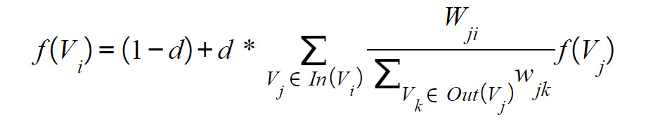
   Figure 7.5: Formula for importance score

   d=0.85 is typically used as the damping factor. While we have used a directed graph here, an undirected graph could also be used with a TextRank algorithm.

5. We repeat the preceding step until the importance score varies by less than a pre-defined tolerance level in two consecutive iterations.
6. Sort the nodes in decreasing order of the importance scores.
7. The top n nodes give us a summary.

The number of iterations required for convergence depends on the number of nodes and the connectedness among the nodes. The number of iterations required for an undirected graph is expected to be higher than the number of iterations required for a directed graph since the edges don't have a direction in the case of the former. We typically use a directed graph in the TextRank algorithm. In general, around 20-40 iterations may be required for convergence. We can drop edges that have less than a certain threshold weight for faster convergence since they won't have much of an impact on the result anyway. The basic concept underpinning the TextRank algorithm is that key parts of a document are connected to form a coherent summary.

Key Input Parameters for TextRank

We'll be using the gensim library to implement TextRank. The following are the parameters required for this:

• text: This is the input text.
• ratio: This is the required ratio of the number of sentences in the summary to the number of sentences in the input text.

The gensim implementation of the TextRank algorithm uses BM25—a probabilistic variation of TF-IDF—for similarity computation in place of the similarity measure described in step 3 of the algorithm. This will be clearer in the following exercise, in which you will summarize text using TextRank.

Exercise 7.02: Performing Summarization Using TextRank

In this exercise, we will use the classic short story, After Twenty Years by O. Henry, which is available on Project Gutenberg, and the first section of the Wikipedia article on Oscar Wilde. We will summarize each text separately so that we have 20% of the sentences in the original text and then have 25% of the sentences in the original text using the gensim implementation of the TextRank algorithm. In all, we shall extract and print four summaries.

In addition to these libraries, you will need to import the following:

from gensim.summarization import summarize

summarize(text,ratio=0.20)

In the preceding code snippet, ratio=0.20 means that 20% of the sentences from the original text will be used to create the summary.

Note

The text corpus for O. Henry's short story, After Twenty Years, being used in this exercise can be found at https://packt.live/33atvr0.

The Oscar Wilde section from the Wikipedia article can be found at https://packt.live/3fhEocY.

Complete the following steps to implement this exercise:

1. Open a Jupyter notebook.
2. Insert a new cell and add the following code to import the necessary libraries and extract the required text from After Twenty Years:

   from gensim.summarization import summarize

   import wikipedia

   import re

   file_url_after_twenty=r'../data/ohenry/pg2776.txt'

   with open(file_url_after_twenty, 'r') as f:

           contents = f.read()

   start_string='AFTER TWENTY YEARS '

   end_string=' LOST ON DRESS PARADE'

   text_after_twenty=contents[contents.find(start_string):

                              contents.find(end_string)]

   text_after_twenty=text_after_twenty.replace(' ',' ')

   text_after_twenty=re.sub(r"s+"," ",text_after_twenty)

   text_after_twenty

   The preceding code generates the following output:

   

   Figure 7.6: Text from After Twenty Years

3. Add the following code to extract the required text and print the summarized text, with the ratio parameter set to 0.2:

   summary_text_after_twenty=summarize(text_after_twenty,

                                       ratio=0.2)

   print(summary_text_after_twenty)

   The preceding code generates the following output:

   

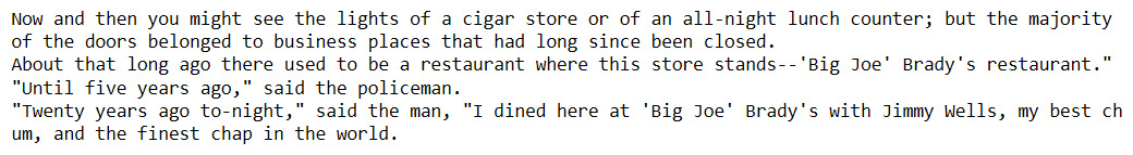
   Figure 7.7: Summarized text when the ratio parameter is 0.2

4. Insert a new cell and add the following code to summarize the text and print the summarized text, with the ratio parameter set to 0.25:

   summary_text_after_twenty=summarize(text_after_twenty,

                                       ratio=0.25)

   print(summary_text_after_twenty)

   The preceding code generates the following output:

   

   Figure 7.8: Summarized text when the ratio parameter is 0.25

5. Insert a new cell and add the following code to extract the required text from the Wikipedia page for Oscar Wilde:

   #text_wiki_oscarwilde=wikipedia.summary("Oscar Wilde")

   file_url_wiki_oscarwilde=r'../data/oscarwilde/'

                             'ow_wikipedia_sum.txt'

   with open(file_url_wiki_oscarwilde, 'r',

             encoding='latin-1') as f:

           text_wiki_oscarwilde = f.read()

   text_wiki_oscarwilde=text_wiki_oscarwilde.replace(' ',' ')

   text_wiki_oscarwilde=re.sub(r"s+"," ",text_wiki_oscarwilde)

   text_wiki_oscarwilde

   The preceding code generates the following output:

   

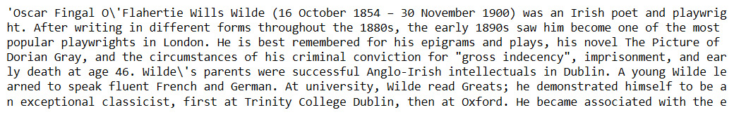
   Figure 7.9: Text from the Wikipedia page for Oscar Wilde

6. Insert a new cell and add the following code to summarize the text and print the summarized text using ratio=0.2:

   summary_wiki_oscarwilde=summarize(text_wiki_oscarwilde,

                                     ratio=0.2)

   print(summary_wiki_oscarwilde)

   The preceding code generates the following output:

   

   Figure 7.10: Summarized text when the ratio parameter is 0.2

7. Add the following code to summarize the text and print the summarized text using ratio=0.25:

   summary_wiki_oscarwilde=summarize(text_wiki_oscarwilde,

                                     ratio=0.25)

   print(summary_wiki_oscarwilde)

   The preceding code generates the following output:

   

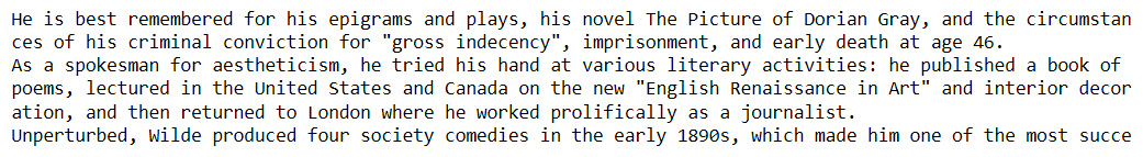
Figure 7.11: Summarized text when the ratio is 0.25

Note

To access the source code for this specific section, please refer to https://packt.live/3i5sNQn.

You can also run this example online at https://packt.live/39G0Knx.

We find that the summary for the Wikipedia article is much more coherent than the short story. We can also see that the summary with a ratio of 0.20 is a subset of a summary with a ratio of 0.25. Would extractive summarization work better for a children's fairytale than it does for an O. Henry short story? Let's explore this in the next exercise.

Exercise 7.03: Summarizing a Children's Fairy Tale Using TextRank

In this exercise, we consider the fairy tale Little Red Riding Hood in two variations for the input texts. The first variation is from Children's Hour with Red Riding Hood and Other Stories, edited by Watty Piper, while the second variation is from The Fairy Tales of Charles Perrault, both of which are available on Project Gutenberg's website. The aim of this exercise is to explore how TextRank (gensim) performs on this summarization.

Note

You can find the text from the Watty Piper variation at https://packt.live/2Xd30xy. The text from the Charles Perrault version can be found at https://packt.live/30g5ZHy.

Complete the following steps to implement this exercise:

1. Open a Jupyter notebook.
2. Insert a new cell and add the following code to import the required libraries:

   from gensim.summarization import summarize

   import re

3. Insert a new cell and add the following code to fetch Watty Piper's version of Little Red Riding Hood:

   file_url_grimms=r'../data/littleredrh/pg11592.txt'

   with open(file_url_grimms, 'r') as f:

           contents_grimms = f.read()

   start_string_grimms='LITTLE RED RIDING HOOD '

   end_string_grimms=' THE GOOSE-GIRL'

   text_grimms=contents_grimms[contents_grimms.find(

                               start_string_grimms):

                               contents_grimms.find(

                               end_string_grimms)]

   text_grimms=text_grimms.replace(' ',' ')

   text_grimms=re.sub(r"s+"," ",text_grimms)

   text_grimms

   The preceding code generates the following output:

   

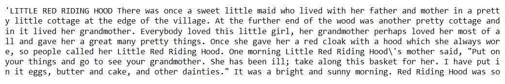
   Figure 7.12: Text from the Watty Piper variation of Little Red Riding Hood

4. Insert a new cell, add the following code, and fetch the Perrault fairy tale version of Little Red Riding Hood:

   file_url_perrault=r'../data/littleredrh/pg29021.txt'

   with open(file_url_perrault, 'r') as f:

           contents_perrault = f.read()

   start_string_perrault='Little Red Riding-Hood '

   end_string_perrault=' _The Moral_'

   text_perrault=contents_perrault[contents_perrault.find(

                                   start_string_perrault):

                                   contents_perrault.find(

                                   end_string_perrault)]

   text_perrault=text_perrault.replace(' ',' ')

   text_perrault=re.sub(r"s+"," ",text_perrault)

   text_perrault

   The preceding code generates the following output:

   

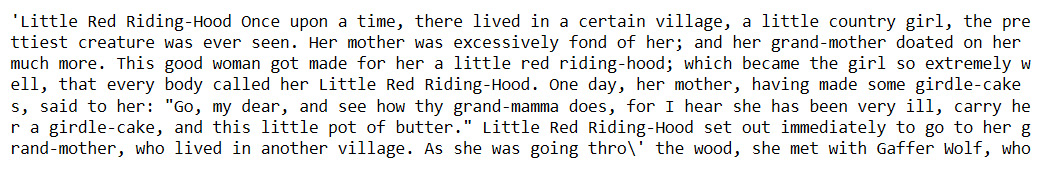
   Figure 7.13: Tales from the Perrault version of Little Red Riding Hood

5. Insert a new cell and add the following code to generate the two summaries with a ratio of 0.20:

   llrh_grimms_textrank=summarize(text_grimms,ratio=0.20)

   llrh_perrault_textrank=summarize(text_perrault,ratio=0.20)

6. Insert a new cell and add the following code to print the TextRank summary (ratio of 0.20) of Grimm's version of Little Red Riding Hood:

   print(llrh_grimms_textrank)

   The preceding code generates the following output:

   

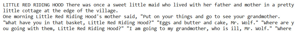
   Figure 7.14: Output after implementing TextRank on the Watty Piper variation

7. Insert a new cell and add the following code to print the TextRank summary (ratio of 0.20) of Perrault's version of Little Red Riding Hood:

   print(llrh_perrault_textrank)

   The preceding code generates the following output:

   

   Figure 7.15: Output after implementing TextRank on the Perrault version

8. Add the following code to generate two summaries with a ratio of 0.5:

   llrh_grimms_textrank=summarize(text_grimms,ratio=0.5)

   llrh_perrault_textrank=summarize(text_perrault,ratio=0.5)

9. Add the following code to print a TextRank summary (ratio of 0.5) of Piper's version of Little Red Riding Hood:

   print(llrh_grimms_textrank)

   The preceding code generates the following output:

   

   Figure 7.16: Output after implementing TextRank on the Watty Piper variation

10. Add the following code to print a TextRank summary (ratio of 0.5) of Perrault's version of Little Red Riding Hood:

    print(llrh_perrault_textrank)

    The preceding code generates the following output:

    

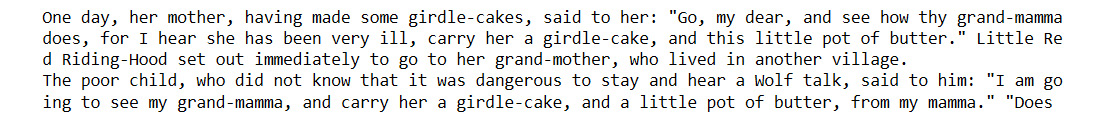
Figure 7.17: Output after implementing TextRank on the Perrault version

Note

To access the source code for this specific section, please refer to https://packt.live/3i5sRzB.

You can also run this example online at https://packt.live/2XfObu1.

With this, we've found that the four summaries lack coherency and are also incomplete. This is also true of the two summaries with a ratio of 0.5—that is, even when half of the sentences are extracted for the summary. This might be because the conversations in the fairytale are contextual in nature, as a sentence often refers to the preceding sentence(s). This contextual aspect of language makes NLP complex for machines.

Interestingly, extractive summarization works much better for an O. Henry short story such as After Twenty Years than it does for a children's fairytale such as Little Red Riding Hood. Furthermore, this is not specific to the language used by a specific author, as we have explored with two different variations of this fairytale. It seems a fairytale is unsuitable for extractive summarization. Lets now do an activity in which we'll use the TextRank algorithm to summarize complaints that customers have written against some organizations.

Activity 7.01: Summarizing Complaints in the Consumer Financial Protection Bureau Dataset

The Consumer Financial Protection Bureau publishes consumer complaints made against organizations in the financial sector. This original dataset is available at https://www.consumerfinance.gov/data-research/consumer-complaints/#download-the-data. To complete this activity, you will summarize a few complaints using TextRank.

Note

You can find the dataset to be used for this activity at https://www.dropbox.com/sh/qmq3x3ah1cf3ecz/AAAg_E6f0I5vdaB4WVmR6TCga?dl=0&preview=Consumer_Complaints.csv. To complete the activity, you will need to place the .csv file into the data folder for this chapter in your local directory.

Follow these steps to implement this activity:

1. Import the summarization libraries and instantiate the summarization model.
2. Load the dataset from a .csv file into a pandas DataFrame. Drop all columns other than Product, Sub-product, Issue, Sub-issue, and Consumer complaint narrative.
3. Select 12 complaints corresponding to the rows 242830, 1086741, 536367, 957355, 975181, 483530, 950006, 865088, 681842, 536367, 132345, and 285894 from the 300,000 odd complaints with a narrative. Note that since the dataset is an evolving dataset, the use of a version that's different from the one in the data folder could give different results because the input texts could be different.
4. Add a column with the TextRank summary. Each element of this column corresponds to a summary, using TextRank, of the complaint narrative in the corresponding column. Use a ratio of 0.20. Also, use a try-except clause since the gensim implementation of the TextRank algorithm throws exceptions with summaries that have very few sentences.
5. Show the DataFrame. You should get an output similar to the following figure:
   

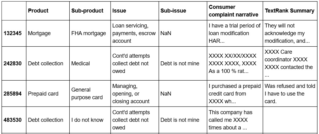
Figure 7.18: DataFrame showing the summarized complaints

Note

The full solution to this activity can be found on page 409.

Recent Developments in Text Generation and Summarization

Alan Turing (for whom the equivalent of the Nobel Prize in Computer Science is named) proposed a test for artificial intelligence in 1950. This test, known as the Turing Test, says that if humans ask questions and cannot distinguish between text responses generated by a machine and a human, then that machine can be deemed to be intelligent.

Text generation using very large models, such as the GPT-2 (with around 1.5 billion parameters) and BERT (Bidirectional Encoder Representation from Transformers) (with around 340 million parameters), can aid in auto-completion tasks. Auto-completion presents unique ethical challenges. While it can offer convenience, it can also reinforce biases in the data. This is accentuated by the fact that most user experience layouts can show only a limited number of options. Furthermore, auto-completion can controversially suggest responses that are different from what the sender originally wants to type.

Unfortunately, most use cases for text generation are negative use cases for generating spam and misinformation. Given that the Turing Test may not be passed any time soon, we are clearly nowhere near considering text generation as a proxy for thought within a machine and there is no widely accepted benchmark for text generation.

Since late 2018, with the invention of self-attention, transformers, and BERT, these approaches are generally considered the best way to teach a machine about some of the most challenging NLP tasks. Self-attention is a technique in which a word is combined with other words in its neighborhood by matrix multiplications. Such multiplications are possible because of vector representations of words. Using such combined representations for all the words in a sentence allows us to represent a sentence in a way that captures context. This allows us to build much larger models that have a significantly higher capacity to learn. A transformer is a combination of attention units and includes position information for each word, that is, multiple self-attention layers and position information are used to capture the context better.

BERT is a transformer that learns the sequential structure of a text in both directions, that is, from left to right and from right to left. This is achieved by randomly masking the words while the model is trained, much like how children are often taught a language by using fill-in-the-blanks exercises. Such is the generalized learning of BERT that it can be used even for translation-related tasks, even though it has not been specifically taught translation as a task. BERT and other large models, such as GPT-2, require a huge computing infrastructure, which is generally not available to most people outside of leading universities and the biggest technology corporations. Pre-trained models fill the void in such cases. The TextRank algorithm considers each sentence to be a bag of words. With the advent of BERT, it is possible for us to have a superior sentence representation that captures meaning much better than the bag of words model.

In the case of summarization, even though there is a benchmark called Recall-Oriented Understudy for Gisting Evaluation (ROUGE), summarization is best evaluated qualitatively given that there isn't only one correct way to summarize text. In February 2020, Microsoft's Turing NLG model, which has 17 billion parameters, generated abstractive summaries for three examples, which were shared publicly. However, the model is not publicly available currently and so the results cannot be reproduced.

Furthermore, we don't know how the Microsoft NLG model does with a naïve test such as the Little Red Riding Hood test. In general, extractive summarization of the kind discussed earlier in this chapter is by far the most useful for practitioners compared with the utility of the state-of-the-art technology in text generation and paraphrasing. Due to this, in the next section, we'll largely focus on practical challenges in extractive summarization.

Practical Challenges in Extractive Summarization

Given the rapid pace of development in NLP, it is even more important to use compatible versions of the libraries that we use. Evaluation of a document's suitability for extractive summarization can be undertaken manually. Often, we would like to summarize multiple pieces of text, all of which could be short in length. The TextRank algorithm will not work well in such cases.

All unverified claims reported in this field ought to be taken with a grain of salt until the claim has been verified. Such claims ought to be subjected by practitioners to naïve tests such as the Little Red Riding test. We can only use a model if it works and if the limitations related to scope and any biases are considered.

Summary

In this chapter, we learned about text generation using Markov chains and extractive summarization using the TextRank algorithm. We also explored both the power and limitations of various advanced approaches. In the next chapter, we will learn about sentiment analysis.