
Overview
This chapter introduces you to the various ways in which text can be represented in the form of vectors. You will start by learning why this is important, and the different types of vector representation. You will then perform one-hot encoding on words, using the preprocessing package provided by scikit-learn, and character-level encoding, both manually and using the powerful Keras library. After covering learned word embeddings and pre-trained embeddings, you will use Word2Vec and Doc2Vec for vector representation for Natural Language Processing (NLP) tasks, such as finding the level of similarity between multiple texts.
Introduction
The previous chapters laid a firm foundation for NLP. But now we will go deeper into a key topic—one that gives us surprising insights into how language processing works and how some of the key advances in human-computer interaction are facilitated. At the heart of NLP is the simple trick of representing text as numbers. This helps software algorithms perform the sophisticated computations that are required to understand the meaning of the text.
As we have already discussed in previous chapters, most machine learning algorithms take numeric data as input and do not understand the text as such. We need to represent our text in numeric form so that we can apply different machine learning algorithms and other NLP techniques to it. These numeric representations are called vectors and are also sometimes called word embeddings or simply embeddings.
This chapter begins with a discussion of vectors, how text can be represented as vectors, and how vectors can be composed to represent complex speech. We will walk through the various representations in both directions—learning how to encode text as vectors as well as how to retrieve text from vectors. We will also look at some cutting-edge techniques used in NLP that are based on the idea of representing text as vectors.
What Is a Vector?
The basic mathematical definition of a vector is an object that has both magnitude and direction. In our definition, it is mostly compared with a scalar, which can be defined as an object that has only magnitude. Vectors are also defined as an element in vector space—for example, a point in space with the coordinates (x=4, y=5, z=6) is a vector. Here, we can see the vector dimensions are the geometric coordinates of a point or element in space. However, the vector dimensions can also represent any quantity or property of some element or object in addition to mere geometric coordinates.
As an example, let's say that we're defining the weather at a given place using five features: temperature, humidity, precipitation, wind speed, and air pressure. The units that these would be measured in are Celsius, percentage, centimeters, kilometers per hour (km/h), and millibar (mbar), respectively. The following are the values for two places:

Figure 6.1: Weather indicators at two different places
So, we can represent the weather of these places in vector form as follows:
- Vector for place 1: [25, 50, 1, 18, 1200.0]
- Vector for place 2: [32, 60, 0, 7, 1019.0]
In the preceding representation, the first dimension represents temperature, the second dimension represents humidity, and so on. Note that the order of these dimensions should be consistent among all the vectors.
Similarly, we can also represent text as a vector in which each dimension can represent either the presence or absence of certain metrics. Examples of these are bag of words and TFIDF vectors that we looked at in the previous chapters. There are other techniques as well for vector representation of text—learned word embeddings, for instance. We will discuss all these different techniques in the upcoming sections. These techniques can be broadly classified into two categories:
- Frequency-based embeddings
- Learned word embeddings
Frequency-Based Embeddings
Frequency-based embedding is a technique in which the text is represented in vector form by considering the frequency of the word in a corpus. The techniques that come under this category are the following:
- Bag of words: As we've already seen in Chapter 2, Feature Extraction Methods, bag of words is the technique of converting text into vector or numeric form by representing each sentence or document in a list the length of which is equal to the total number of unique words in the corpus.
- TFIDF: As seen previously in Chapter 2, Feature Extraction Methods, this technique considers the frequency of a term as well as the inverse of its occurrence in the corpus.
- Term frequency-based technique: This is a somewhat simpler version of TFIDF. We represent each word in the vector by its number of occurrences in the document. For example, let's say that a document contains the following sentences:
- The girl is pretty, and the boy is handsome.
- Do whatever your heart says.
- The boy has a bike.
- His bike was red in color.
Now let's build term frequency vectors of all these sentences. We will first create a dictionary of unique words as follows. Note that we are considering every word in lowercase only:
{1: the
2: girl
3: pretty
4: and
5: boy
5: is
7: handsome
8: do
9: whatever
10: your
11: heart
12: says
13: was
14: has
15: bike
16: his
17: red
18: in
19: color
}
Now every document will be represented by a vector with 19 dimensions, where every dimension represents the frequency of a word in that document. So, for sentence 1, the vector will be [2, 1, 1, 1, 1, 2, 1, 0, 0, 0, 0, 0, 0, 0, 0, 0, 0, 0, 0, 0]. Similarly, for sentence 2, the vector representation will be [0, 0, 0, 0, 0, 0, 0, 1, 1, 1, 1, 1, 0, 0, 0, 0, 0, 0, 0, 0], and so on. Note that the order needs to be consistent here, too.
Note
It is recommended that you use preprocessing techniques such as stemming, stop word removal, and conversion to lowercase before converting a text into the aforementioned vector format. Term frequency is a simple and quick technique for converting text into vector form. However, the TFIDF technique is a more effective technique than term frequency as it not only considers the frequency of a word in the current document but also in the background corpus.
- One-hot encoding: In all techniques described previously, we have represented a word with a single number. Using one-hot encoding, we can represent a word with an array. To understand this concept better, let's take the following sentences:
- I love cats and dogs.
- Cats are light in weight.
We will use a dictionary to assign a numeric label or index to each unique word (after converting to lowercase) as follows:
{1: i
2: love
3: cats
4: and
5: dogs
6: are
7: light
8: in
9: weight
}
Now we will represent each word in these sentences as follows:
i [1 0 0 0 0 0 0 0 0]
love [0 1 0 0 0 0 0 0 0]
cats [0 0 1 0 0 0 0 0 0]
and [0 0 0 1 0 0 0 0 0]
dogs [0 0 0 0 1 0 0 0 0]
are [0 0 0 0 0 1 0 0 0]
light [0 0 0 0 0 0 1 0 0]
in [0 0 0 0 0 0 0 1 0]
weight [0 0 0 0 0 0 0 0 1]
We can see that each vector consists of 9 elements; that is, the number of elements equals the total number of words in the dictionary. For each word, the value of an element will be 1, only if the word is present at the corresponding position in the dictionary. When one-hot encoding words, you also need to consider the vocabulary. The meaning of vocabulary here is the total number of unique words in the text sources for your project. So, if you have a large source, then you will end up with a huge vocabulary and large one-hot vector sizes, which will eventually consume a lot of memory. The next exercise on word-level one-hot encoding will help us understand this better.
Label encoding is a technique used to convert categorical data in numerical data, where each category is represented by a unique number. In order to perform label encoding and one-hot encoding, we will be using the LabelEncoder() and OneHotEncoder() classes from the preprocessing package provided by the scikit-learn library. The following exercise will help us get a better understanding of this.
Exercise 6.01: Word-Level One-Hot Encoding
In this exercise, we will one-hot encode words with the help of the preprocessing package provided by the scikit-learn library. For this, we shall make use of a file containing lines from Jane Austen's Pride and Prejudice.
Note
The text file used for this exercise can be found at https://packt.live/3hUxNqQ.
Follow these steps to implement this exercise:
- Open a Jupyter notebook.
- First, load the file containing the lines from the novel using the Path class provided by the pathlib library to specify the location of the file. Insert a new cell and add the following code:
from pathlib import Path
data = Path('../data')
novel_lines_file = data / 'novel_lines.txt'
- Now that you have the file, open it and read its contents. Use the open() and read() functions to perform these actions. Store the results in the novel_lines file variable. Insert a new cell and add the following code to implement this:
with novel_lines_file.open() as f:
novel_lines_raw = f.read()
- After reading the contents of the file, load it by inserting a new cell and adding the following code:
novel_lines_raw
The code generates the following output:
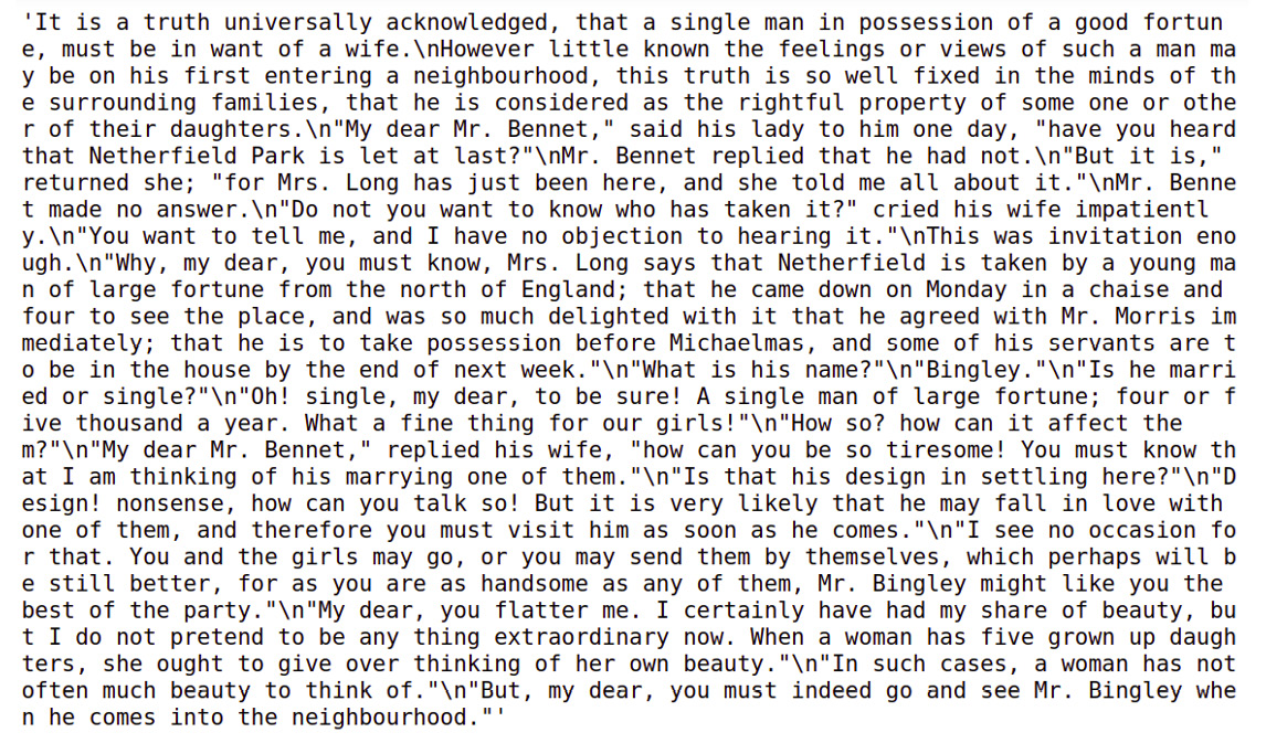
Figure 6.2: Raw text from the file
In the output, you will see a lot of newline characters. This is because we loaded the entire content at once into a single variable instead of separate lines. You will also see a lot of non-alphanumeric characters.
- The main objective is to create one-hot vectors for each word in the file. To do this, construct a vocabulary, which is the entire list of unique words in the file, by tokenizing the string into words and removing newlines and non-alphanumeric characters. Define a function named clean_tokenize() to do this. Store the vocabulary created using clean_tokenize() inside a variable named novel_lines. Add the following code:
import string
import re
alpha_characters = str.maketrans('', '', string.punctuation)
def clean_tokenize(text):
text = text.lower()
text = re.sub(r' ', '*** ', text)
text = text.translate(alpha_characters)
text = re.sub(r' +', ' ', text)
return text.split(' ')
novel_lines = clean_tokenize(novel_lines_raw)
- Take a look at the content inside novel_lines now. It should look like a list. Insert a new cell and add the following code to view it:
novel_lines
The code generates the following output:

Figure 6.3: Text after preprocessing is done
- Insert a new cell and add the following code to convert the list to a NumPy array and print the shape of the array:
import numpy as np
novel_lines_array = np.array([novel_lines])
novel_lines_array = novel_lines_array.reshape(-1, 1)
novel_lines_array.shape
The code generates the following output:
(459, 1)
As you can see, the novel_lines_array array consists of 459 rows and 1 column. Each row is a word in the original novel_lines file.
Note
NumPy arrays are more specific to NLP algorithms than Python lists. It is the format that is required for the scikit-learn library, which we will be using to one-hot encode words.
- Now use encoders, such as the LabelEncoder() and OneHotEncoder() classes from scikit-learn's preprocessing package, to convert novel_lines_array to one-hot encoded format. Insert a new cell and add the following lines of code to implement this:
from sklearn import preprocessing
labelEncoder = preprocessing.LabelEncoder()
novel_lines_labels = labelEncoder.fit_transform(
novel_lines_array)
import warnings
warnings.filterwarnings('ignore')
wordOneHotEncoder = preprocessing.OneHotEncoder()
line_onehot = wordOneHotEncoder.fit_transform(
novel_lines_labels.reshape(-1,1))
In the code, the LabelEncoder() class encodes the labels, and the fit_transform() method fits the label encoder and returns the encoded labels.
- To check the list of encoded labels, insert a new cell and add the following code:
novel_lines_labels
The preceding code generates output that looks as follows:

Figure 6.4: List of encoded labels
The OneHotEncoder() class encodes the categorical integer features as a one-hot numeric array. The fit_transform() method of this class takes the novel_lines_labels array as input. This is a numeric array, and each feature included in this array is encoded using the one-hot encoding scheme.
- Create a binary column for each category. A sparse matrix is returned as output. To view the matrix, insert a new cell and type the following code:
line_onehot
The code generates the following output:
<459x199 sparse matrix of type '<class 'numpy.float64'>'
With 459 stored elements in Compressed Sparse Row format>
- To convert the sparse matrix into a dense array, use the toarray() function. Insert a new cell and add the following code to implement this:
line_onehot.toarray()
The code generates the following output:
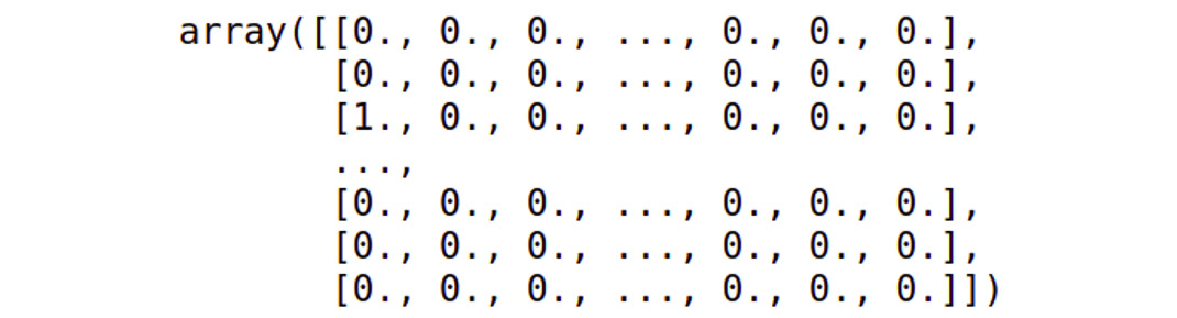
Figure 6.5: Dense array
Note
To access the source code for this specific section, please refer to https://packt.live/2Xd2aAU.
You can also run this example online at https://packt.live/39GSAeu.
The preceding output shows that we have achieved our objective of one-hot encoding words.
One-hot encoding is mostly used in techniques such as language generation models, where a model is trained to predict the next word in the sequence given the words that precede it (think about your phone recommending words while you're chatting with your friends). Language models are used in many important natural language tasks nowadays, including machine translation, spell correction, text summarization, and in tools like Amazon Echo, Alexa, and more.
In addition to word-level language models, we can also build character-level language models, which can be trained to predict the next character in a sequence of characters. For character-level language models, we need character-level one-hot encoding. Let's explore this in the next section.
Character-Level One-Hot Encoding
In character-level one-hot encoding, we assign a numeric value to all the possible characters. We can use alpha-numeric characters and punctuation as well. Then, we represent each character by an array of size equal to all the characters in the document. This array contains zero at all the indices, other than the index assigned with the character. Let's explain this with an example. Consider the word "hello". Let's say our vocabulary contains only twenty-six characters, so our dictionary will look like this:
{'a': 0
'b': 1
'c': 2
'd': 3
'e': 4
'f': 5
'g': 6
'h': 7
'i': 8
'j': 9
'k': 10
…….'z': 25}
Now, 'h' will be represented as [0 0 0 0 0 0 0 1 0 0 0 0 0 0 0 0 0 0 0 0 0 0 0 0 0 0 0]. Similarly, 'e' can be represented as [0 0 0 0 1 0 0 0 0 0 0 0 0 0 0 0 0 0 0 0 0 0 0 0 0 0]. Let's see how we can implement this in the next exercise.
Exercise 6.02: Character One-Hot Encoding – Manual
In this exercise, we will create our own function that can one-hot encode the characters of the word "data". Follow these steps to complete this exercise:
- Open a Jupyter notebook.
- To one-hot encode the characters of a given word, create a function named onehot_word(). Within this function, create a lookup table for each of the characters in the given word. Then, map each character to an index. Add the following code to implement this:
def onehot_word(word):
lookup = {v[1]: v[0] for v in enumerate(set(word))}
word_vector = []
- Next, loop through the characters in the word and create a vector named one_hot_vector of the same size as the number of characters in the lookup. This vector is filled with zeros. Then, use the lookup table to find the position of the character and set that character's value to 1.
Note
Execute the code for step 1 and step 2 together.
Add the following code:
for c in word:
one_hot_vector = [0] * len(lookup)
one_hot_vector[lookup[c]] = 1
word_vector.append(one_hot_vector)
return word_vector
The function created earlier will return a word vector.
- Once the onehot_word() function has been created, test it by adding some input as a parameter. Add the word "data" as an input to the function. To implement this, add a new cell and write the following code:
onehot_vector = onehot_word('data')
print(onehot_vector)
The code generates the following output:
[0, 0, 1], [1, 0, 0], [0, 1, 0], [1, 0, 0]
Since there are four characters in the input (data), there will be four one-hot vectors. To determine the size of each one-hot vector for data, we enumerate the total number of characters in it. It is important to note that only one index gets assigned for repeated characters. After enumerating through the characters, the character d will be assigned index 0, the character a will be assigned index 1, and the character t will be assigned index 2.
Based on each character's index position, the elements in each one-hot vector will be marked as 1, leaving other elements marked 0. In this way, we can manually one-hot encode any given text. Note that, in most practical applications, the size of one-hot encoded vector is equal to the size of all the characters, and sometimes, non-alphabetical characters are also considered.
Note
To access the source code for this specific section, please refer to https://packt.live/314aTX1.
You can also run this example online at https://packt.live/3gaWbE5.
We have learned how character-level one-hot encoding can be performed manually by developing our own function. We will focus on performing character-level one-hot encoding using Keras in the next exercise. Keras is a machine learning library that works along with TensorFlow to create deep learning models.
We will be using the Tokenizer class from Keras to create vectors from the text. Tokenizer can work on both characters and words, depending on the char_level argument. If char_level is set to true, then it will work on the character level; otherwise, it will work on the word level. The Tokenizer class comes with the following functions:
- fit_on_text(): This method reads all the text and creates an internal dictionary, either word-wise or character-wise. We should always call it for the entire text, so that no word or character is left out of the dictionary. All the methods/variables listed after this should be called or used only after calling this method.
- word_index: This is a dictionary that contains all the possible words or characters in the vocabulary. Each word or character is assigned a unique number/index.
- index_word: This is the reverse dictionary of word_index; it contains key-value pairs with the index as the key and the word or character as its value.
- texts_to_sequences(): This function converts each word or character sequence into its corresponding index value.
- texts_to_matrix(): This converts each word or character in a given text into one-hot vector using a built-in dictionary. It takes the text as input, processes it, and returns a NumPy array of one-hot encoded vectors.
Exercise 6.03: Character-Level One-Hot Encoding with Keras
In this exercise, we will perform one-hot encoding on a given word using the Keras library. Follow these steps to implement this exercise:
- Open a Jupyter notebook.
- Insert a new cell and the following code to import the necessary libraries:
from keras.preprocessing.text import Tokenizer
import numpy as np
- Once you have imported the Tokenizer class, create an instance of it by inserting a new cell and adding the following code:
char_tokenizer = Tokenizer(char_level=True)
Since you are encoding at the character level, in the constructor, char_level is set to True.
Note
By default, char_level is set to False if we are encoding words.
- To test the Tokenizer instance, you will require some text to work on. Insert a new cell and add the following code to assign a string to the text variable:
text = 'The quick brown fox jumped over the lazy dog'
- After getting the text, use the fit_on_texts() method provided by the Tokenizer class. Insert a new cell and add the following code to implement this:
char_tokenizer.fit_on_texts(text)
In this code, char_tokenizer will break text into characters and internally keep track of the tokens, the indices, and everything else needed to perform one-hot encoding.
- Now, look at the possible output. One type of output is the sequence of the characters—that is, the integers assigned with each character in the text. The texts_to_sequences() method of the Tokenizer class helps assign integers to each character in the text. Insert a new cell and add the following code to implement this:
seq =char_tokenizer.texts_to_sequences(text)
seq
The code generates the following output:

Figure 6.6: List of integers assigned to each character
As you can see, there were 44 characters in the text variable. From the output, we can see that for every unique character in text, an integer is assigned.
- Use sequences_to_texts() to get text from the sequence with the following code:
char_tokenizer.sequences_to_texts(seq)
The snippet of the preceding output follows:

Figure 6.7: Text generated from the sequence
- Now look at the actual one-hot encoded values. For this, use the texts_to_matrix() function. Insert a new cell and add the following code to implement this:
char_vectors = char_tokenizer.texts_to_matrix(text)
Here, the results of the array are stored in the char_vectors variable.
- In order to view the vector values, just insert a new cell and add the following line:
char_vectors
On execution, the code displays the array of one-hot encoded vectors:

Figure 6.8: Actual one-hot encoded values for the given text
- In order to investigate the dimensions of the NumPy array, make use of the shape attribute. Insert a new cell and add the following code to execute it:
char_vectors.shape
The following output is generated:
(44, 27)
So, char_vectors is a NumPy array with 44 rows and 27 columns. This is because we are considering 26 characters and an additional character for space.
- To access the first row of char_vectors NumPy array, insert a new cell and add the following code:
char_vectors[0]
This returns a one-hot vector, which can be seen in the following figure:
array([0 ., 0., 0., 0., 1., 0., 0., 0., 0 .,
0., 0., 0., 0., 0., 0., 0.,0., 0 .,
0., 0., 0., 0., 0., 0., 0 ., 0., 0])
- To access the index of this one-hot vector, use the argmax() function provided by NumPy. Insert a new cell and write the following code to implement this:
np.argmax(char_vectors[0])
The code generates the following output:
4
- The Tokenizer class provides two dictionaries, index_word and word_index, which you can use to view the contents of Tokenizer in key-value form. Insert a new cell and add the following code to view the index_word dictionary:
char_tokenizer.index_word
The code generates the following output:

Figure 6.9: The index_word dictionary
As you can see in this figure, the indices act as keys, and the characters act as values. Now insert a new cell and the following code to view the word_index dictionary:
char_tokenizer.word_index
The code generates the following output:
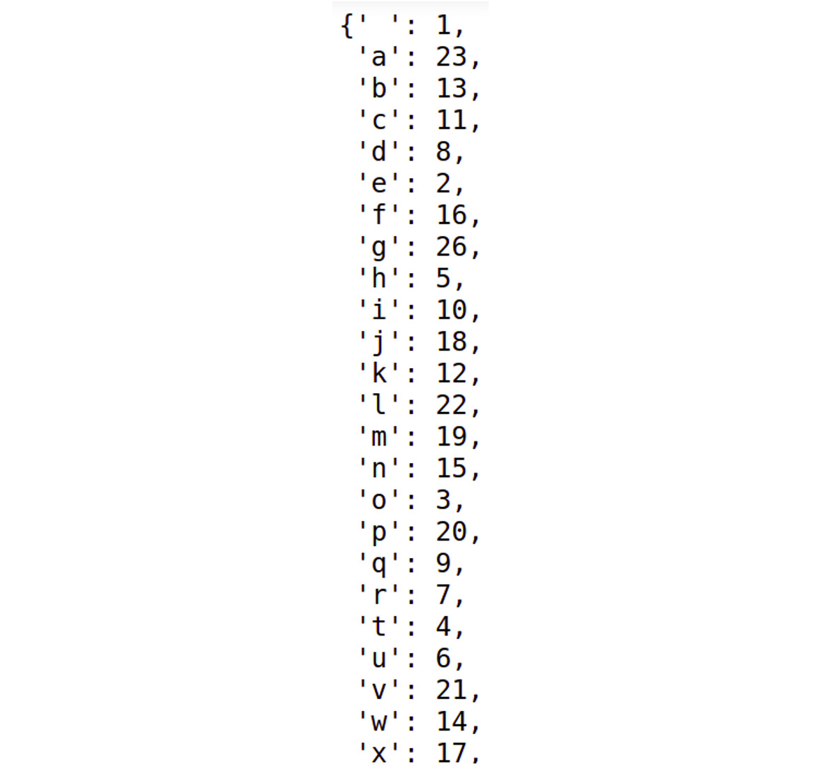
Figure 6.10: The word_index dictionary
In this figure, the characters act as keys, and the indices act as values.
- In the preceding steps, you saw how to access the index of a given one-hot vector by using the argmax() function provided by NumPy. Using this index as a key, you can access its value in the index_word dictionary. To implement this, we insert a new cell and write the following code:
char_tokenizer.index_word[np.argmax(char_vectors[0])]
The preceding code generates the following output:
't'
In this code, np.argmax(char_vectors[0]) produces an output of 4. This will act as a key in finding the value in the index_word dictionary. So, when char_tokenizer.index_word[4] is executed, it will scan through the dictionary and find that, for key 4, the value is t, and finally, it will print t.
Note
To access the source code for this specific section, please refer to https://packt.live/2ECjNnf.
You can also run this example online at https://packt.live/2P9c69V.
In the preceding section, we learned how to convert text into one-hot vectors at either the character level or the word level. One-hot encoding is a simple representation of a word, but it has a disadvantage. Whenever the corpus is large (that is, when the number of unique characters or words increases), the size of the one-hot encoded vector also increases. Thus, it becomes very memory intensive and is sometimes not feasible; speed and simplicity here lead to the "curse of dimensionality" by creating a new dimension for each category/word. To tackle this problem, learned embeddings can be used, as explained in the following sections.
Learned Word Embeddings
The vector representations discussed in the preceding section have some serious disadvantages, as discussed here:
- Sparsity and large size: The sizes of one-hot encoded or other frequency-based vectors depend upon the number of unique words in the corpus. This means that when the size of the corpus increases, the number of unique words increases, thereby increasing the size of the vectors in turn.
- Context: None of these vector representations consider the words with respect to its context while representing it as a vector. However, the meaning of a word in any language depends upon the context it is used in. Not taking the context into account can often lead to inaccurate results.
Prediction-based word embeddings or learned word embeddings try to address both problems. For starters, these methods represent words with a fixed number of dimensions. Moreover, these representations are actually learned from the different contexts in which the word has been used at different places. Learned word embeddings is actually a collective name given to a set of language models that represent words in such a way that words with similar meanings have somewhat similar representations. There are different techniques for creating learned word embeddings, such as Word2Vec and GloVe. Let's discuss them one by one.
Word2Vec
Word2Vec is a prediction-based algorithm that represents a word by a vector of a fixed size. This is a form of unsupervised learning algorithm, which means that we need not to provide manually annotated data; we just feed the raw text. It will train a model in such a way that each word is represented in terms of its context throughout the training data.
This algorithm has two variations, as follows:
- Continuous Bag of Words (CBoW): This model tends to predict the probability of a word given the context. The learning problem here is to predict the word given a fixed-window context—that is, a fixed set of continuous words in text.
- Skip-Gram model: This model is the reverse of the CBoW model, as it tends to predict the context of a word.
These vectors find application in a lot of NLP tasks including text generation, machine translation, speech to text, text to speech, text classification, and text similarity.
Let's explore how they can be used for text similarity. Suppose we generated 300 dimensional vectors from words such as "love", "adorable", and "hate". If we find the cosine similarity between the vectors for "love" and "adorable", and "love" and "hate", we will find a higher similarity between the former pair of words than the latter.
In the next exercise, we will train word vectors using the gensim library. Specifically, we'll be using the Word2Vec class. The Word2Vec class has parameters such as documents, size, window, min_count, and workers. Here, documents refers to the sentences that we have to provide to the class, size represents the length of the dense vector to represent each token, min_count represents the minimum count of words that can be taken into consideration when training a particular model, and workers represents the number of threads that are required when training a model.
For training a model, we use the model.train() method. This method takes arguments such as documents, total_examples, and epochs. Here, documents represents the sentences, and total_examples represents the count of sentences, while epochs represents the total number of iterations over the given data. Finally, the trained word vectors get stored in model.wv, which is an instance of KeyedVectors.
In order to perform basic text cleaning, before it's processed, we will make use of the textcleaner class from gensim. Some of the most useful functions available in textcleaner that we will be using are as follows:
- split_sentences(): As the name suggests, this function splits the text and gets a list of sentences from the text.
- simple_preprocess(): This function converts a document into a list consisting of lowercase tokens.
Let's see how we can use these functions to create word vectors.
Exercise 6.04: Training Word Vectors
In this exercise, we will train word vectors. We will be using books freely available on Project Gutenberg for this. We will also see the vector representation using Matplotlib's pyplot framework.
Note
The file we are using for this exercise can be found at https://packt.live/39JeZYP.
Follow these steps to implement this exercise:
- Open a Jupyter notebook.
- Use the requests library to load books from the Project Gutenberg website, the json library to load a book catalog, and the regex package to clean the text by removing newline characters. Insert a new cell and add the following code to implement this:
import requests
import json
import re
- After importing all the necessary libraries, load the json file, which contains details of 10 books, including the title, the author, and the ID. Insert a new cell and add the following steps to implement this:
with open('../data/ProjectGutenbergBooks.json', 'r')
as catalog_file:
catalog = json.load(catalog_file)
- To print the details of all the books, insert a new cell and add the following code:
catalog
The preceding code generates the following output:
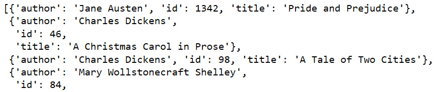
Figure 6.11: Book details in the catalog
- Create a function named load_book(), which will take book_id as a parameter and, based on that book_id, fetch the book and load it. It should also clean the text by removing the newline characters. Insert a new cell and add the following code to implement this:
GUTENBERG_URL ='https://www.gutenberg.org/files/{}/{}-0.txt'
def load_book(book_id):
url = GUTENBERG_URL.format(book_id, book_id)
contents = requests.get(url).text
cleaned_contents = re.sub(r' ', ' ', contents)
return cleaned_contents
- Once you have defined our load_book() function, you will loop through the catalog, fetch all the id instances of the books, and store them in the book_ids list. The id instances stored in the book_ids list will act as parameters for our load_book() function. The book information fetched for each book ID will be loaded in the books variable. Insert a new cell and add the following code to implement this:
book_ids = [ book['id'] for book in catalog ]
books = [ load_book(id) for id in book_ids]
To view the information of the books variable, add the following code in a new cell:
books[:5]
A snippet of the output generated by the preceding code is as follows:

Figure 6.12: Information of various books
- Before you can train the word vectors, you need to split the books into a list of documents. In this case, you want to teach the Word2Vec algorithm about words in the context of the sentences that they are in. So here, a document is actually a sentence. Thus, you need to create a list of sentences from all 10 books. Insert a new cell and add the following code to implement this:
from gensim.summarization import textcleaner
from gensim.utils import simple_preprocess
def to_sentences(book):
sentences = textcleaner.split_sentences(book)
sentence_tokens = [simple_preprocess(sentence)
for sentence in sentences]
return sentence_tokens
In the preceding code, all the text preprocessing takes place inside the to_sentences() function that you have defined.
- Now, loop through each book in books and pass each book as a parameter to the to_sentences() function. The results should be stored in the book_sentences variable. Also, split books into sentences and sentences into documents. The result should be stored in the documents variable. Insert a new cell and add the following code to implement this:
books_sentences = [to_sentences(book) for book in books]
documents = [sentence for book_sent in books_sentences
for sentence in book_sent]
- To check the length of the documents, use the len() function as follows:
len(documents)
The code generates the following output:
32922
- Now that you have your documents, train the model by making use of the Word2Vec class provided by the gensim package. Insert a new cell and add the following code to implement this:
from gensim.models import Word2Vec
# build vocabulary and train model
model = Word2Vec(
documents,
size=100,
window=10,
min_count=2,
workers=10)
model.train(documents, total_examples=len(documents),
epochs=50)
The code generates the following output:
(27809439, 37551450)
Now make use of the most_similar() function of the model.wv instance to find the similar words. The most_similar() function takes positive as a parameter and returns a list of strings that contribute positively. Insert a new cell and add the following code to implement this:
model.wv.most_similar(positive="worse")
The code generates the following output:
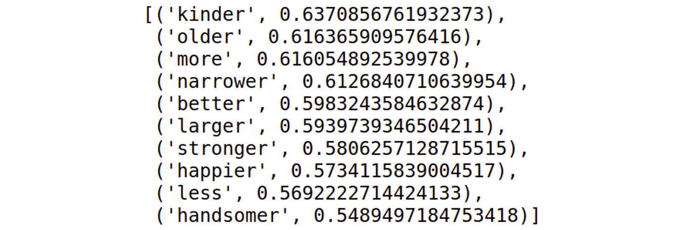
Figure 6.13: Most similar words
Note
You may get a slightly different output as the output depends on the model training process, so you may have a different model than the one we have trained here.
- Create a show_vector() function that will display the vector using pyplot, a plotting framework in Matplotlib. Insert a new cell and add the following code to implement this:
%matplotlib inline
import matplotlib.pyplot as plt
def show_vector(word):
vector = model.wv[word]
fig, ax = plt.subplots(1,1, figsize=(10, 2))
ax.tick_params(axis='both',
which='both',
left=False,
bottom=False,
top=False,
labelleft=False,
labelbottom=False)
ax.grid(False)
print(word)
ax.bar(range(len(vector)), vector, 0.5)
show_vector('sad')
The code generates the following output:

Figure 6.14: Graph of the vector when the input is "sad"
Note
To access the source code for this specific section, please refer to https://packt.live/317nb11.
You can also run this example online at https://packt.live/2BJC40I.
In the preceding figure, we can see the vector representation when the word provided to the show_vector() function is "sad". We have learned about training word vectors and representing them using pyplot. In the next section, we will focus more on using pre-trained word vectors, which are required for NLP projects.
Using Pre-Trained Word Vectors
For a machine learning model, the more data you have, the better the model you get. But training the model on large amounts of data is intensively resource-consuming in terms of both time and memory. So, we usually train a Word2Vec model on a large amount of data and retain the model for future use. There are also a lot of pre-trained models publicly available have been trained on huge datasets such as Wikipedia articles. These models include gensim by fastText (research group by Facebook), and Word2Vec has recently proved to be state-of-the-art for tasks including checking for word analogies and word similarities, as follows:
- vector('Paris') - vector('France') + vector('Italy') results in a vector that is very close to vector('Rome').
- vector('king') - vector('man') + vector('woman') is close to vector('queen').
Google's publicly available glove model is similar to the Word2Vec model and has produced incredible results. In some applications, we may need to train a Word2Vec model on our own specific dataset rather than train a new model from scratch; that is, we can train a pre-trained model on more data. This process is called transfer learning. Transfer learning is based on the concept of transferring knowledge from one domain into another.
Note
Pre-trained word vectors can get pretty large. For example, vectors trained on Google News contain 3 million words, and on disk, its compressed size is 1.5 GB.
To better understand how we can use pre-trained word vectors in Python, let's walk through a simple exercise.
Exercise 6.05: Using Pre-Trained Word Vectors
In this exercise, we will load and use pre-trained word embeddings. We will also show the image representation of a few word vectors using the pyplot framework of the Matplotlib library. We will be using glove6B50d.txt, which is a pre-trained model.
Note
The pre-trained model being used for this file can be found at https://www.kaggle.com/watts2/glove6b50dtxt/download. Download this file and place it in the data folder of Chapter 6, Vector Representation.
Follow these steps to complete this exercise:
- Open a Jupyter notebook.
- Add the following statement to import the numpy library:
import numpy as np
import zipfile
- Move the downloaded model from the preceding link to the location given in the following code snippet. In order to extract data from a ZIP file, use the zipfile Python package. Add the following code to unzip the embeddings from the ZIP file:
GLOVE_DIR = '../data/'
GLOVE_ZIP = GLOVE_DIR + 'glove6B50d.txt.zip'
print(GLOVE_ZIP)
zip_ref = zipfile.ZipFile(GLOVE_ZIP, 'r')
zip_ref.extractall(GLOVE_DIR)
zip_ref.close()
- Define a function named load_glove_vectors() to return a model Python dictionary. Insert a new cell and add the following code to implement this:
def load_glove_vectors(fn):
print("Loading Glove Model")
with open( fn,'r', encoding='utf8') as glove_vector_file:
model = {}
for line in glove_vector_file:
parts = line.split()
word = parts[0]
embedding = np.array([float(val)
for val in parts[1:]])
model[word] = embedding
print("Loaded {} words".format(len(model)))
return model
glove_vectors = load_glove_vectors(GLOVE_DIR +'glove6B50d.txt')
Here, glove_vector_file is a text file containing a dictionary. In this, words act as keys and vectors act as values. So, we need to read the file line by line, split it, and then map it to a Python dictionary. The preceding code generates the following output:
Loading Glove Model
Loaded 400000 words
If we want to view the values of glove_vectors, then we insert a new cell and add the following code:
glove_vectors
You will get the following output:
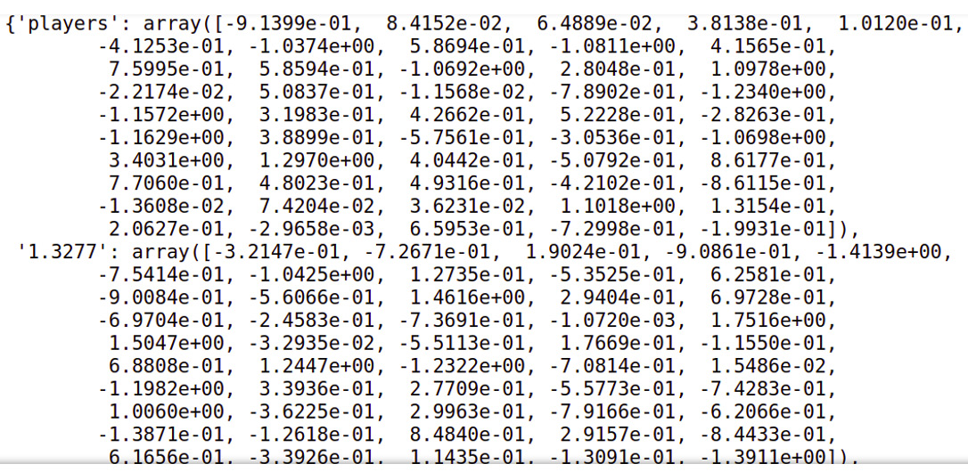
Figure 6.15: Dictionary of glove_vectors
The order of the result dictionary can vary as it is a Python dict.
- The glove_vectors object is basically a dictionary containing the mappings of the words to the vectors, so you can access the vector for a word, which will return a 50-dimensional vector. Insert a new cell and add the code to check the vector for the word dog:
glove_vectors["dog"]

Figure 6.16: Array of glove vectors with an input of dog
In order to see the vector for the word cat, add the following code:
glove_vectors["cat"]
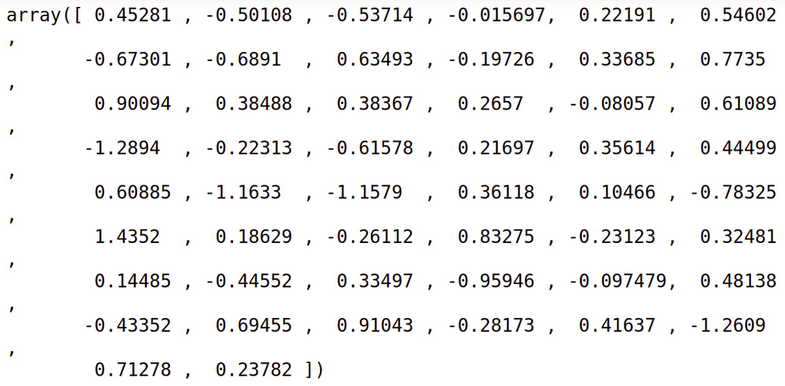
Figure 6.17: Array of glove vectors with an input of cat
- Now that you have the vectors, represent them as an image using the pyplot framework of the Matplotlib library. Insert a new cell and add the following code to implement this:
import matplotlib.pyplot as plt
def to_vector(glove_vectors, word):
vector = glove_vectors.get(word.lower())
if vector is None:
vector = [0] * 50
return vector
def to_image(vector, word=''):
fig, ax = plt.subplots(1,1)
ax.tick_params(axis='both', which='both',
left=False,
bottom=False,
top=False,
labelleft=False,
labelbottom=False)
ax.grid(False)
ax.bar(range(len(vector)), vector, 0.5)
ax.text(s=word, x=1, y=vector.max()+0.5)
return vector
In the preceding code, you defined two functions. The to_vector() function accepts glove_vectors and word as parameters. Here, the get() function of glove_vectors will find the word and convert it into lowercase. The result will be stored in the vector variable.
- The to_image() function takes vector and word as input and shows the image representation of vector. To find the image representation of the word man, type the following code:
man = to_image(to_vector(glove_vectors, "man"))
The code generates the following output:

Figure 6.18: Graph generated with an input of man
- To find the image representation of the word woman, type the following code:
woman = to_image(to_vector(glove_vectors, "woman"))
This will generate the following output:
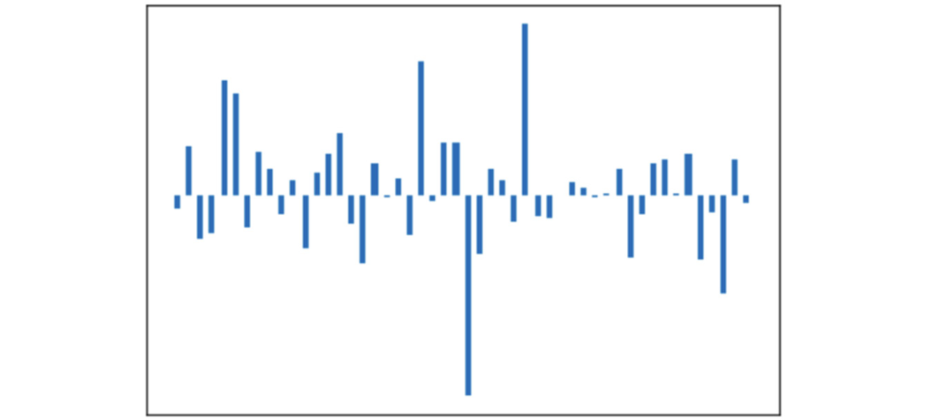
Figure 6.19: Graph generated with an input of woman
- To find the image representation of the word king, type the following code:
king = to_image(to_vector(glove_vectors, "king"))
This will generate the following output:

Figure 6.20: Graph generated with an input of king
- To find the image representation of the word queen, type the following code:
queen = to_image(to_vector(glove_vectors, "queen"))
This will generate the following output:
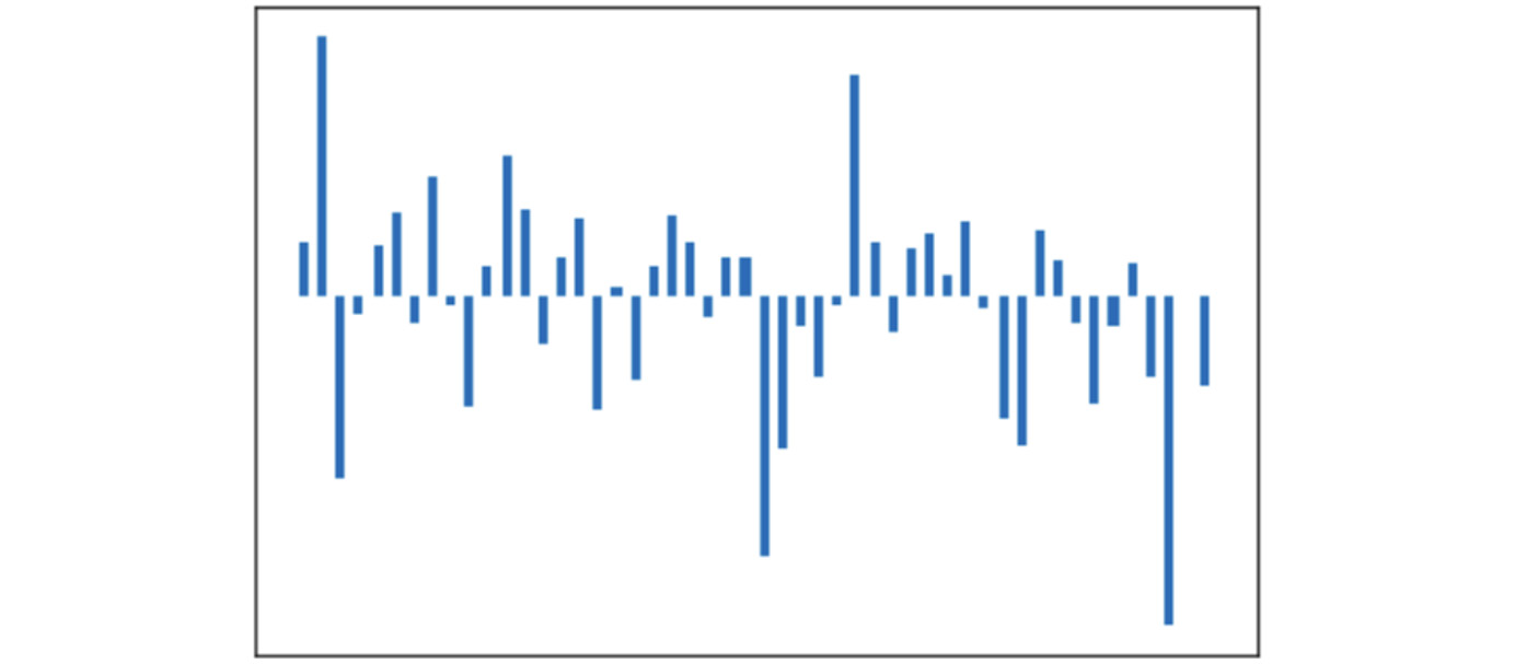
Figure 6.21: Graph generated with an input of queen
- To find the image representation of the vector for king – man + woman – queen, type the following code:
diff = to_image(king – man + woman - queen)
This will generate the following output:

Figure 6.22: Graph generated with (king-man+woman-queen) as input
- To find the image representation of the vector for king – man + woman, type the following code:
nd = to_image(king – man + woman)
This will generate the following output:

Figure 6.23: Graph generated with (king-man+woman) as input
Note
To access the source code for this specific section, please refer to https://packt.live/33btLpH.
This section does not currently have an online interactive example, and will need to be run locally.
The preceding results are the visual proof of the example we already discussed. We've learned how to load and use pre-trained word vectors and view their image representations. In the next section, we will focus on document vectors and their uses.
Document Vectors
Word vectors and word embeddings represent words. But if we wanted to represent a whole document, we'd need to use document vectors. Note that when we refer to a document, we are referring to a collection of words that have some meaning to a user. A document can be a single sentence or a group of sentences. A document can consist of product reviews, tweets, or lines of movie dialogue, and can be from a few words to thousands of words. A document can be used in a machine learning project as an instance of something that the algorithm can learn from. We can represent a document with different techniques:
- Calculating the mean value: We calculate the mean of all the constituent word vectors of a document and represent the document by the mean vector.
- Doc2Vec: Doc2Vec is a technique by which we represent documents by a fixed-length vector. It is trained quite similarly to the way we train the Word2Vec model. Here, we also add the unique ID of the document to which the word belongs. Then, we can get the vector of the document from the trained model using the document ID.
Similar to Word2Vec, the Doc2Vec class contains parameters such as min_count, window, vector_size, sample, negative, and workers. The min_count parameter ignores all the words with a frequency less than that specified. The window parameter sets the maximum distance between the current and predicted words in the given sentence. The vector_size parameter sets the dimensions of each vector.
The sample parameter defines the threshold that allows us to configure the higher-frequency words that are regularly down-sampled, while negative specifies the total amount of noise words that should be drawn and workers specifies the total number of threads required to train the model. To build the vocabulary from the sequence of sentences, Doc2Vec provides the build_vocab method. We'll be using all of these in the upcoming exercise.
Uses of Document Vectors
Some of the uses of document vectors are as follows:
- Similarity: We can use document vectors to compare texts for similarity. For example, legal AI software can use document vectors to find similar legal cases.
- Recommendations: For example, online magazines can recommend similar articles based on those that users have already read.
- Predictions: Document vectors can be used as input into machine learning algorithms to build predictive models.
In the next section, we will perform an exercise based on document vectors.
Exercise 6.06: Converting News Headlines to Document Vectors
In this exercise, we will convert some news headlines into document vectors. Also, we will look at the image representation of the vector. Again, for image representation, we will be using the pyplot framework of the Matplotlib library. Follow these steps to complete this exercise:
Note
The file which we are going to use in this exercise is in zipped format and can be found at https://packt.live/3fhE2TG. It should be unzipped once downloaded.
- Open a Jupyter notebook.
- Import all the necessary libraries for this exercise. You will be using the gensim library. Insert a new cell and add the following code:
import pandas as pd
from gensim import utils
from gensim.models.doc2vec import TaggedDocument
from gensim.models import Doc2Vec
from gensim.parsing.preprocessing
import preprocess_string, remove_stopwords
import random
import warnings
warnings.filterwarnings("ignore")
In the preceding code snippet, other than other imports, you imported TaggedDocument from gensim, which prepares the document formats used in Doc2Vec. It represents the document along with the tag. This will be clearer from the following code lines. Doc2Vec requires each instance to be a TaggedDocument instance.
- Move the downloaded file to the following location and create a variable of the path as follows:
sample_news_data = '../data/sample_news_data.txt'
- Now load the file:
with open(sample_news_data, encoding="utf8",
errors='ignore') as f:
news_lines = [line for line in f.readlines()]
- Now create a DataFrame out of the headlines as follows:
lines_df = pd.DataFrame()
indices = list(range(len(news_lines)))
lines_df['news'] = news_lines
lines_df['index'] = indices
- View the head of the DataFrame using the following code:
lines_df.head()
This will create the following output:
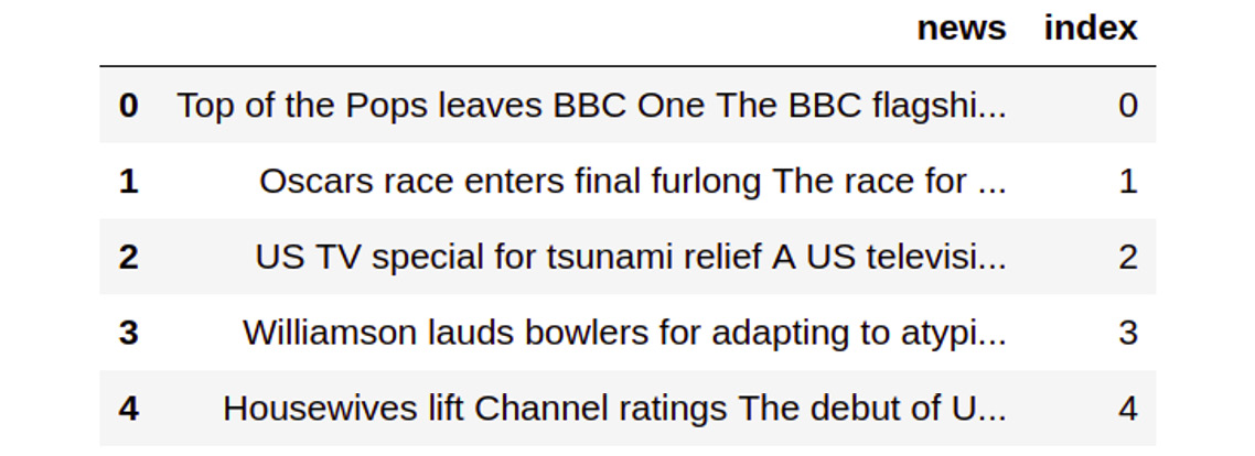
Figure 6.24: Head of the DataFrame
- Create a class, the object of which will create the training instances for the Doc2Vec model. Insert a new cell and add the following code to implement this:
class DocumentDataset(object):
def __init__(self, data:pd.DataFrame, column):
document = data[column].apply(self.preprocess)
self.documents = [ TaggedDocument( text, [index])
for index, text in
document.iteritems() ]
def preprocess(self, document):
return preprocess_string(
remove_stopwords(document))
def __iter__(self):
for document in self.documents:
yield documents
def tagged_documents(self, shuffle=False):
if shuffle:
random.shuffle(self.documents)
return self.documents
In the code, the preprocess_string() function applies the given filters to the input. As its name suggests, the remove_stopwords() function is used to remove stopwords from the given document. Since Doc2Vec requires each instance to be a TaggedDocument instance, we create a list of TaggedDocument instances for each headline in the file.
- Create an object of the DocumentDataset class. It takes two parameters. One is the lines_df_small DataFrame and the other is the Line column name. Insert a new cell and add the following code to implement this:
documents_dataset = DocumentDataset(lines_df, 'news')
- Create a Doc2Vec model using the Doc2Vec class. Insert a new cell and add the following code to implement this:
docVecModel = Doc2Vec(min_count=1, window=5, vector_size=100,
sample=1e-4, negative=5, workers=8)
docVecModel.build_vocab(documents_dataset.tagged_documents())
- Now you need to train the model using the train() function of the Doc2Vec class. This could take a while, depending on how many records we train. Here, epochs represents the total number of records required to train the document. Insert a new cell and add the following code to implement this:
docVecModel.train(documents_dataset.
tagged_documents(shuffle=True),
total_examples = docVecModel.corpus_count,
epochs=10)
- Save this model for future use as follows:
docVecModel.save('../data/docVecModel.d2v')
- The model has been trained. To verify this, access one of the vectors with its index. To do this, insert a new cell and add the following code to find the doc vector of index 657:
docVecModel[657]
You should get an output similar to the one below:
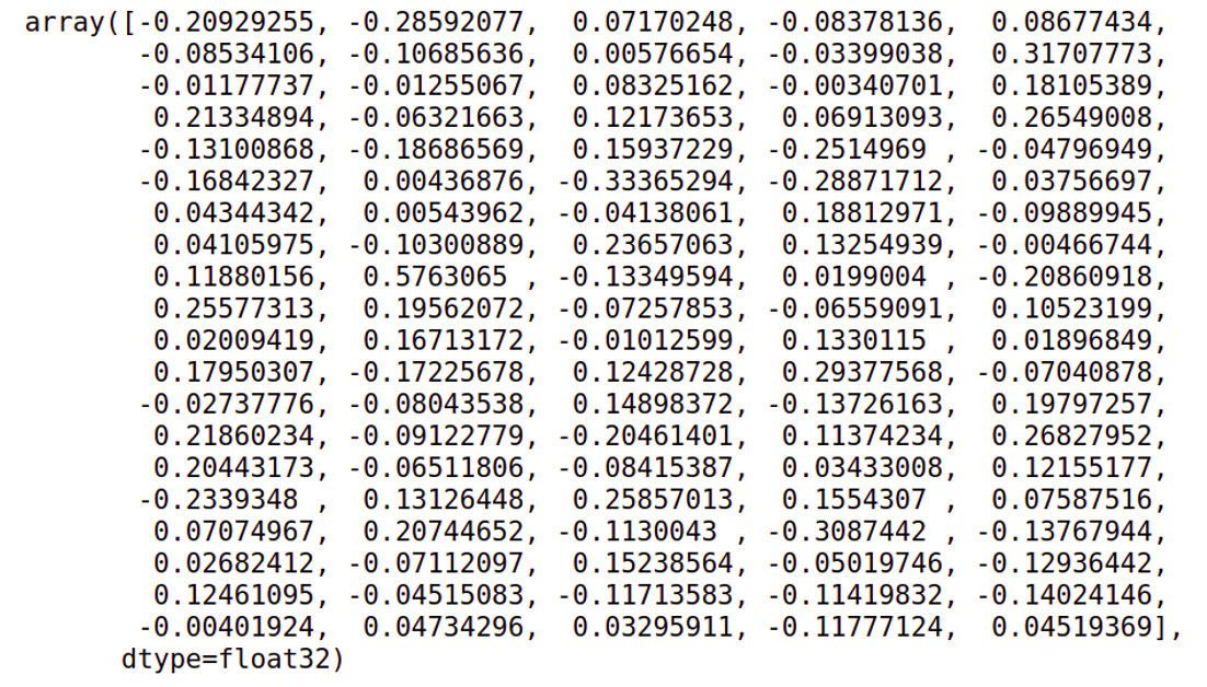
Figure 6.25: Lines represented as vectors
- To check the image representation of any given vector, make use of the pyplot framework of the Matplotlib library. The show_news_lines() function takes a line number as a parameter. Based on this line number, find the vector and store it in the doc_vector variable. The show_image() function takes two parameters, vector and line, and displays an image representation of the vector. Insert a new cell and add the following code to implement this:
import matplotlib.pyplot as plt
def show_image(vector, line):
fig, ax = plt.subplots(1,1, figsize=(10, 2))
ax.tick_params(axis='both',
which='both',
left=False,
bottom=False,
top=False,
labelleft=False,
labelbottom=False)
ax.grid(False)
print(line)
ax.bar(range(len(vector)), vector, 0.5)
def show_news_lines(line_number):
line = lines_df[lines_df.index==line_number].news
doc_vector = docVecModel[line_number]
show_image(doc_vector, line)
- Now that you have defined the functions, implement the show_news_lines() function to view the image representation of the vector. Insert a new cell and add the following code to implement this:
show_news_lines(872)
The code generates the following output:
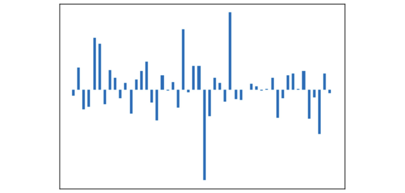
Figure 6.26: Image representation of a given vector
Note
To access the source code for this specific section, please refer to https://packt.live/30dFxxV.
You can also run this example online at https://packt.live/39MiTQG.
We have learned how to represent a document as a vector. We have also seen a visual representation of this. In the next section, we will complete an activity to find similar news headlines using the document vector.
Activity 6.01: Finding Similar News Article Using Document Vectors
To complete this activity, you need to build a news search engine that finds similar news articles like the one provided as input using the Doc2Vec model. You will find headlines similar to "US raise TV indecency US politicians are proposing a tough new law aimed at cracking down on indecency." Follow these steps to complete this activity:
- Open a Jupyter notebook and import the necessary libraries.
- Load the new article lines file.
- Iterate over each headline and split the columns and create a DataFrame.
- Load the Doc2Vec model that you created in the previous exercise.
- Create a function that converts the sentences into vectors and another that does the similarity checks.
- Test both the functions.
Note
The full solution to this activity can be found on page 406.
So, in this activity, we were able to find similar news headlines with the help of document vectors. A common use case of inferring text similarity from document vectors is in text paraphrasing, which we'll explore in detail in the next chapter.
Summary
In this chapter, we learned about the motivations behind converting human language in the form of text into vectors. This helps machine learning algorithms to execute mathematical functions on the text, detect patterns in language, and gain an understanding of the meaning of the text. We also saw different types of vector representation techniques, such as character-level encoding and one-hot encoding.
In the next chapter, we will look at the areas of text paraphrasing, summarization, and generation. We will see how we can automate the process of text summarization using the NLP techniques we have learned so far.