
Overview
In this chapter, you will be able to categorize data based on its content and structure. You will be able to describe preprocessing steps in detail and implement them to clean up text data. You will learn about feature engineering and calculate the similarity between texts. Once you understand these concepts, you will be able to use word clouds and some other techniques to visualize text.
Introduction
In the previous chapter, we learned about the concepts of Natural Language Processing (NLP) and text analytics. We also took a quick look at various preprocessing steps. In this chapter, we will learn how to make text understandable to machine learning algorithms.
As we know, to use a machine learning algorithm on textual data, we need a numerical or vector representation of text data since most of these algorithms are unable to work directly with plain text or strings. But before converting the text data into numerical form, we will need to pass it through some preprocessing steps such as tokenization, stemming, lemmatization, and stop-word removal.
So, in this chapter, we will learn a little bit more about these preprocessing steps and how to extract features from the preprocessed text and convert them into vectors. We will also explore two popular methods for feature extraction (Bag of Words and Term Frequency-Inverse Document Frequency), as well as various methods for finding similarity between different texts. By the end of this chapter, you will have gained an in-depth understanding of how text data can be visualized.
Types of Data
To deal with data effectively, we need to understand the various forms in which it exists. First, let's explore the types of data that exist. There are two main ways to categorize data (by structure and by content), as explained in the upcoming sections.
Categorizing Data Based on Structure
Data can be divided on the basis of structure into three categories, namely, structured, semi-structured, and unstructured data, as shown in the following diagram:
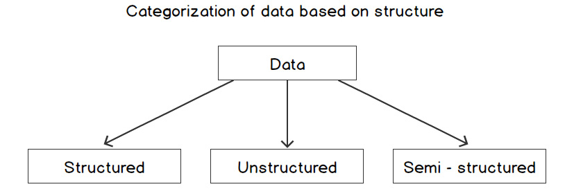
Figure 2.1: Categorization based on content
These three categories are as follows:
- Structured data: This is the most organized form of data. It is represented in tabular formats such as Excel files and Comma-Separated Value (CSV) files. The following image shows what structured data usually looks like:

Figure 2.2: Structured data
The preceding table contains information about five people, with each row representing a person and each column representing one of their attributes.
- Semi-structured data: This type of data is not presented in a tabular structure, but it can be transformed into a table. Here, information is usually stored between tags following a definite pattern. XML and HTML files can be referred to as semi-structured data. The following screenshot shows how semi-structured data can appear:
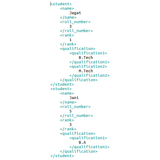
Figure 2.3: Semi-structured data
The format shown in the preceding screenshot is called markup language format. Here, the data is stored between tags, hierarchically. It is a universally accepted format, and there are a lot of parsers available that can convert this data into structured data.
- Unstructured data: This type of data is the most difficult to deal with. Machine learning algorithms would find it difficult to comprehend unstructured data without any loss of information. Text corpora and images are examples of unstructured data. The following image shows what unstructured data looks like:

Figure 2.4: Unstructured data
This is called unstructured data because if we want to get employee details from the preceding text snippet with our program, we will not be able to do so by simple parsing. We have to make our algorithm understand the semantics of the language to make it able to extract information from this.
Categorizing Data Based on Content
Data can be divided into four categories based on content, as shown in the following diagram:

Figure 2.5: Categorizing data based on structure
Let's look at each category here:
- Text data: This refers to text corpora consisting of written sentences. This type of data can only be read. An example would be the text corpus of a book.
- Image data: This refers to pictures that are used to communicate messages. This type of data can only be seen.
- Audio data: This refers to voice recordings, music, and so on. This type of data can only be heard.
- Video data: A continuous series of images coupled with audio forms a video. This type of data can be seen as well as heard.
With that, we have learned about the different types of data and their categorization on the basis of structure and content. When dealing with unstructured data, it is necessary to clean it first. In the next section, we will look into some of the preprocessing steps for cleaning data.
Cleaning Text Data
The text data that we are going to discuss here is unstructured text data, which consists of written sentences. Most of the time, this text data cannot be used as it is for analysis because it contains some noisy elements, that is, elements that do not really contribute much to the meaning of the sentence at all. These noisy elements need to be removed because they do not contribute to the meaning and semantics of the text. If they're not removed, they can not only waste system memory and processing time, but also negatively impact the accuracy of the results. Data cleaning is the art of extracting meaningful portions from data by eliminating unnecessary details. Consider the sentence, "He tweeted, 'Live coverage of General Elections available at this.tv/show/ge2019. _/\_ Please tune in :) '. "
In this example, to perform NLP tasks on the sentence, we will need to remove the emojis, punctuation, and stop words, and then change the words into their base grammatical form.
To achieve this, methods such as stopword removal, tokenization, and stemming are used. We will explore them in detail in the upcoming sections. Before we do so, let's get acquainted with some basic NLP libraries that we will be using here:
- Re: This is a standard Python library that's used for string searching and string manipulation. It contains methods such as match(), search(), findall(), split(), and sub(), which are used for basic string matching, searching, replacing, and more, using regular expressions. A regular expression is nothing but a set of characters in a specific order that represents a pattern. This pattern is searched for in the texts.
- textblob: This is an open source Python library that provides different methods for performing various NLP tasks such as tokenization and PoS tagging. It is similar to nltk, which was introduced in Chapter 1, Introduction to Natural Language Processing. It is built on the top of nltk and is much simpler as it has an easier to use interface and excellent documentation. In projects that don't involve a lot of complexity, it should be preferable to nltk.
- keras: This is an open source, high-level neural network library that's was developed on top of another neural network library called TensorFlow. In addition to neural network functionality, it also provides methods for basic text processing and NLP tasks.
Tokenization
Tokenization and word tokenizers were briefly described in Chapter 1, Introduction to Natural Language Processing. Tokenization is the process of splitting sentences into their constituents; that is, words and punctuation. Let's perform a simple exercise to see how this can be done using various packages.
Exercise 2.01: Text Cleaning and Tokenization
In this exercise, we will clean some text and extract the tokens from it. Follow these steps to complete this exercise:
- Open a Jupyter Notebook.
- Import the re package:
import re
- Create a method called clean_text() that will delete all characters other than digits, alphabetical characters, and whitespaces from the text and split the text into tokens. For this, we will use the text which matches with all non-alphanumeric characters, and we will replace all of them with an empty string:
def clean_text(sentence):
return re.sub(r'([^sw]|_)+', ' ', sentence).split()
- Store the sentence to be cleaned in a variable named sentence and pass it through the preceding function. Add the following code to this: implement
sentence = 'Sunil tweeted, "Witnessing 70th Republic Day "
"of India from Rajpath, New Delhi. "
"Mesmerizing performance by Indian Army! "
"Awesome airshow! @india_official "
"@indian_army #India #70thRepublic_Day. "
"For more photos ping me [email protected] :)"'
clean_text(sentence)
The preceding command fragments the string wherever any blank space is present. The output should be as follows:
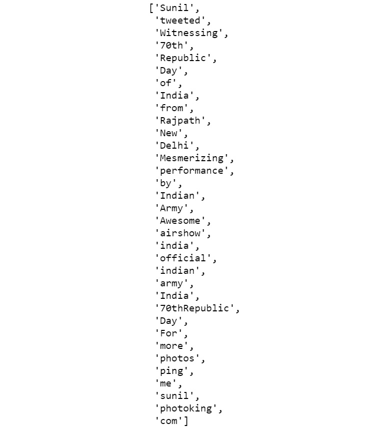
Figure 2.6: Fragmented string
With that, we have learned how to extract tokens from text. Often, extracting each token separately does not help. For instance, consider the sentence, "I don't hate you, but your behavior." Here, if we process each of the tokens, such as "hate" and "behavior," separately, then the true meaning of the sentence would not be comprehended. In this case, the context in which these tokens are present becomes essential. Thus, we consider n consecutive tokens at a time. n-grams refers to the grouping of n consecutive tokens together.
Note
To access the source code for this specific section, please refer to https://packt.live/2CQikt7.
You can also run this example online at https://packt.live/33cn0nF.
Next, we will look at an exercise where n-grams can be extracted from a given text.
Exercise 2.02: Extracting n-grams
In this exercise, we will extract n-grams using three different methods. First, we will use custom-defined functions, and then the nltk and textblob libraries. Follow these steps to complete this exercise:
- Open a Jupyter Notebook.
- Import the re package and create a custom-defined function, which we can use to extract n-grams. Add the following code to do this:
import re
def n_gram_extractor(sentence, n):
tokens = re.sub(r'([^sw]|_)+', ' ', sentence).split()
for i in range(len(tokens)-n+1):
print(tokens[i:i+n])
In the preceding function, we are splitting the sentence into tokens using regex, then looping over the tokens, taking n consecutive tokens at a time.
- If n is 2, two consecutive tokens will be taken, resulting in bigrams. To check the bigrams, we pass the function the text and with n=2. Add the following code to do this:
n_gram_extractor('The cute little boy is playing with the kitten.',
2)
The preceding code generates the following output:
['The', 'cute']
['cute', 'little']
['little', 'boy']
['boy', 'is']
['is', 'playing']
['playing', 'with']
['with', 'the']
['the', 'kitten']
- To check the trigrams, we pass the function with the text and with n=3. Add the following code to do this:
n_gram_extractor('The cute little boy is playing with the kitten.',
3)
The preceding code generates the following output:
['The', 'cute', 'little']
['cute', 'little', 'boy']
['little', 'boy', 'is']
['boy', 'is', 'playing']
['is', 'playing', 'with']
['playing', 'with', 'the']
['with', 'the', 'kitten']
- To check the bigrams using the nltk library, add the following code:
from nltk import ngrams
list(ngrams('The cute little boy is playing with the kitten.'
.split(), 2))
The preceding code generates the following output:
[('The', 'cute'),
('cute', 'little'),
('little', 'boy'),
('boy', 'is'),
('is', 'playing'),
('playing', 'with'),
('with', 'the'),
('the', 'kitten')]
- To check the trigrams using the nltk library, add the following code:
list(ngrams('The cute little boy is playing with the kitten.'.split(), 3))
The preceding code generates the following output:
[('The', 'cute', 'little'),
('cute', 'little', 'boy'),
('little', 'boy', 'is'),
('boy', 'is', 'playing'),
('playing', 'with', 'the'),
('with', 'the', 'kitten.')]
- To check the bigrams using the textblob library, add the following code:
!pip install -U textblob
from textblob import TextBlob
blob = TextBlob("The cute little boy is playing with the kitten.")
blob.ngrams(n=2)
The preceding code generates the following output:
[WordList(['The', 'cute']),
WordList(['cute', 'little']),
WordList(['little', 'boy']),
WordList(['boy', 'is']),
WordList(['is', 'playing']),
WordList(['playing', 'with']),
WordList(['with', 'the']),
WordList(['the', 'kitten'])]
- To check the trigrams using the textblob library, add the following code:
blob.ngrams(n=3)
The preceding code generates the following output:
[WordList(['The', 'cute', 'little']),
WordList(['cute', 'little', 'boy']),
WordList(['little', 'boy', 'is']),
WordList(['boy', 'is' 'playing']),
WordList(['is', 'playing' 'with']),
WordList(['playing', 'with' 'the']),
WordList(['with', 'the' 'kitten'])]
In this exercise, we learned how to generate n-grams using various methods.
Note
To access the source code for this specific section, please refer to https://packt.live/2PabHUK.
You can also run this example online at https://packt.live/2XbjFRX.
Exercise 2.03: Tokenizing Text with Keras and TextBlob
In this exercise, we will use keras and textblob to tokenize texts. Follow these steps to complete this exercise:
- Open a Jupyter Notebook and insert a new cell.
- Import the keras and textblob libraries and declare a variable named sentence, as follows.
from keras.preprocessing.text import text_to_word_sequence
from textblob import TextBlob
sentence = 'Sunil tweeted, "Witnessing 70th Republic Day "
"of India from Rajpath, New Delhi. "
"Mesmerizing performance by Indian Army! "
"Awesome airshow! @india_official "
"@indian_army #India #70thRepublic_Day. "
"For more photos ping me [email protected] :)"'
- To tokenize using the keras library, add the following code:
def get_keras_tokens(text):
return text_to_word_sequence(text)
get_keras_tokens(sentence)
The preceding code generates the following output:

Figure 2.7: Tokenization using Keras
- To tokenize using the textblob library, add the following code:
def get_textblob_tokens(text):
blob = TextBlob(text)
return blob.words
get_textblob_tokens(sentence)
The preceding code generates the following output:

Figure 2.8: Tokenization using textblob
With that, we have learned how to tokenize texts using the keras and textblob libraries.
Note
To access the source code for this specific section, please refer to https://packt.live/3393hFi.
You can also run this example online at https://packt.live/39Dtu09.
In the next section, we will discuss the different types of tokenizers.
Types of Tokenizers
There are different types of tokenizers that come in handy for specific tasks. Let's look at the ones provided by nltk one by one:
- Whitespace tokenizer: This is the simplest type of tokenizer. It splits a string wherever a space, tab, or newline character is present.
- Tweet tokenizer: This is specifically designed for tokenizing tweets. It takes care of all the special characters and emojis used in tweets and returns clean tokens.
- MWE tokenizer: MWE stands for Multi-Word Expression. Here, certain groups of multiple words are treated as one entity during tokenization, such as "United States of America," "People's Republic of China," "not only," and "but also." These predefined groups are added at the beginning with mwe() methods.
- Regular expression tokenizer: These tokenizers are developed using regular expressions. Sentences are split based on the occurrence of a specific pattern (a regular expression).
- WordPunctTokenizer: This splits a piece of text into a list of alphabetical and non-alphabetical characters. It actually splits text into tokens using a fixed regex, that is, 'w+|[^ws]+'.
Now that we have learned about the different types of tokenizers, in the next section, we will carry out an exercise to get a better understanding of them.
Exercise 2.04: Tokenizing Text Using Various Tokenizers
In this exercise, we will use different tokenizers to tokenize text. Perform the following steps to implement this exercise:
- Open a Jupyter Notebook.
- Insert a new cell and the following code to import all the tokenizers and declare a variable sentence:
from nltk.tokenize import TweetTokenizer
from nltk.tokenize import MWETokenizer
from nltk.tokenize import RegexpTokenizer
from nltk.tokenize import WhitespaceTokenizer
from nltk.tokenize import WordPunctTokenizer
sentence = 'Sunil tweeted, "Witnessing 70th Republic Day "
"of India from Rajpath, New Delhi. "
"Mesmerizing performance by Indian Army! "
"Awesome airshow! @india_official "
"@indian_army #India #70thRepublic_Day. "
"For more photos ping me [email protected] :)"'
- To tokenize the text using TweetTokenizer, add the following code:
def tokenize_with_tweet_tokenizer(text):
# Here will create an object of tweetTokenizer
tweet_tokenizer = TweetTokenizer()
"""
Then we will call the tokenize method of
tweetTokenizer which will return token list of sentences.
"""
return tweet_tokenizer.tokenize(text)
tokenize_with_tweet_tokenizer(sentence)
Note
The # symbol in the code snippet above denotes a code comment. Comments are added into code to help explain specific bits of logic.
The preceding code generates the following output:
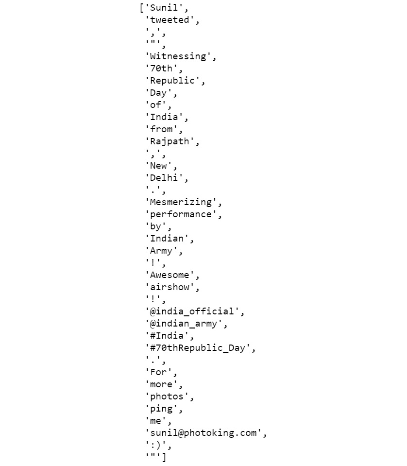
Figure 2.9: Tokenization using TweetTokenizer
As you can see, the hashtags, emojis, websites, and Twitter IDs are extracted as single tokens. If we had used the white space tokenizer, we would have got hash, dots, and the @ symbol as separate tokens.
- To tokenize the text using MWETokenizer, add the following code:
def tokenize_with_mwe(text):
mwe_tokenizer = MWETokenizer([('Republic', 'Day')])
mwe_tokenizer.add_mwe(('Indian', 'Army'))
return mwe_tokenizer.tokenize(text.split())
tokenize_with_mwe(sentence)
The preceding code generates the following output:
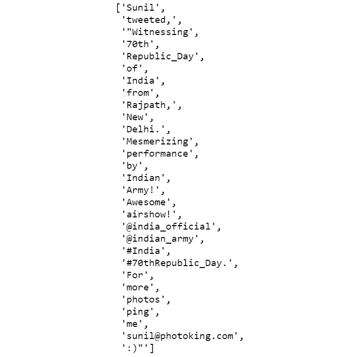
Figure 2.10: Tokenization using the MWE tokenizer
In the preceding screenshot, the words "Indian" and "Army!", which should have been treated as a single identity, were treated separately. This is because "Army!" (not "Army") is treated as a token. Let's see how this can be fixed in the next step.
- Add the following code to fix the issues in the previous step:
tokenize_with_mwe(sentence.replace('!',''))
The preceding code generates the following output:

Figure 2.11: Tokenization using the MWE tokenizer after removing the "!" sign
Here, we can see that instead of being treated as separate tokens, "Indian" and "Army" are treated as a single entity.
- To tokenize the text using the regular expression tokenizer, add the following code:
def tokenize_with_regex_tokenizer(text):
reg_tokenizer = RegexpTokenizer('w+|$[d.]+|S+')
return reg_tokenizer.tokenize(text)
tokenize_with_regex_tokenizer(sentence)
The preceding code generates the following output:
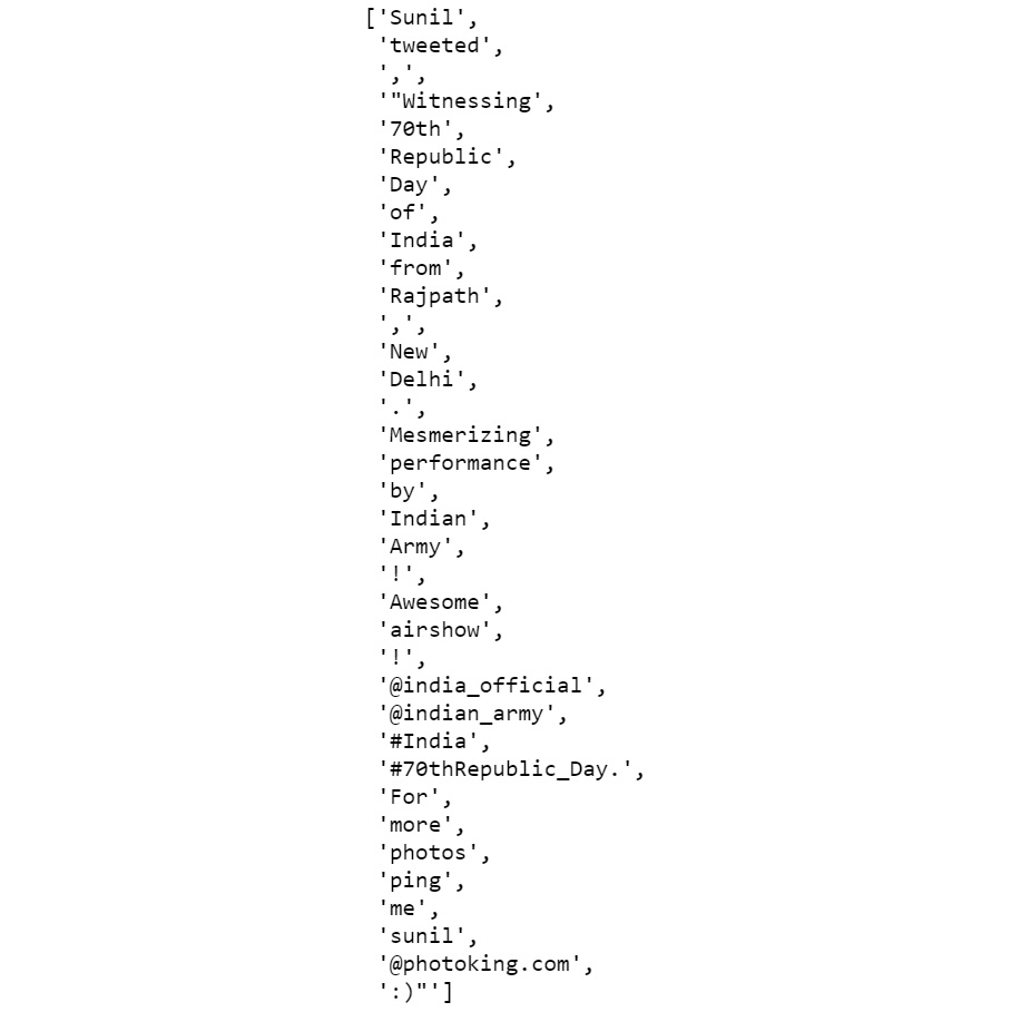
Figure 2.12: Tokenization using the regular expression tokenizer
- To tokenize the text using the whitespace tokenizer, add the following code:
def tokenize_with_wst(text):
wh_tokenizer = WhitespaceTokenizer()
return wh_tokenizer.tokenize(text)
tokenize_with_wst(sentence)
The preceding code generates the following output:

Figure 2.13: Tokenization using the whitespace tokenizer
- To tokenize the text using the Word Punct tokenizer, add the following code:
def tokenize_with_wordpunct_tokenizer(text):
wp_tokenizer = WordPunctTokenizer()
return wp_tokenizer.tokenize(text)
tokenize_with_wordpunct_tokenizer(sentence)
The preceding code generates the following output:

Figure 2.14: Tokenization using the Word Punct tokenizer
In this section, we have learned about different tokenization techniques and their nltk implementation.
Note
To access the source code for this specific section, please refer to https://packt.live/3hSbDWi.
You can also run this example online at https://packt.live/3hOi7oR.
Now, we're ready to use them in our programs.
Stemming
In many languages, the base forms of words change when they're used in sentences. For example, the word "produce" can be written as "production" or "produced" or even "producing," depending on the context. The process of converting a word back into its base form is known as stemming. It is essential to do this, because without it, algorithms would treat two or more different forms of the same word as different entities, despite them having the same semantic meaning. So, the words "producing" and "produced" would be treated as different entities, which can lead to erroneous inferences. In Python, RegexpStemmer and PorterStemmer are the most widely used stemmers. Let's explore them one at a time.
RegexpStemmer
RegexpStemmer uses regular expressions to check whether morphological or structural prefixes or suffixes are present. For instance, in many cases, verbs in the present continuous tense (the present tense form ending with "ing") can be restored to their base form simply by removing "ing" from the end; for example, "playing" becomes "play".
Let's complete the following exercise to get some hands-on experience with RegexpStemmer.
Exercise 2.05: Converting Words in the Present Continuous Tense into Base Words with RegexpStemmer
In this exercise, we will use RegexpStemmer on text to convert words into their basic form by removing some generic suffixes such as "ing" and "ed". To use nltk's regex_stemmer, we have to create an object of RegexpStemmer by passing the regex of the suffix or prefix and an integer, min, which indicates the minimum length of the stemmed string. Follow these steps to complete this exercise:
- Open a Jupyter Notebook.
- Insert a new cell and import RegexpStemmer:
from nltk.stem import RegexpStemmer
- Use regex_stemmer to stem each word of the sentence variable. Add the following code to do this:
def get_stems(text):
"""
Creating an object of RegexpStemmer, any string ending
with the given regex 'ing$' will be removed.
"""
regex_stemmer = RegexpStemmer('ing$', min=4)
"""
The below code line will convert every word into its
stem using regex stemmer and then join them with space.
"""
return ' '.join([regex_stemmer.stem(wd) for
wd in text.split()])
sentence = "I love playing football"
get_stems(sentence)
The preceding code generates the following output:
'I love play football'
As we can see, the word playing has been changed into its base form, play. In this exercise, we learned how we can perform stemming using nltk's RegexpStemmer.
Note
To access the source code for this specific section, please refer to https://packt.live/3hRYUm6.
You can also run this example online at https://packt.live/2D0Ztvk.
The Porter Stemmer
The Porter stemmer is the most common stemmer for dealing with English words. It removes various morphological and inflectional endings (such as suffixes, prefixes, and the plural "s") from English words. In doing so, it helps us extract the base form of a word from its variations. To get a better understanding of this, let's carry out a simple exercise.
Exercise 2.06: Using the Porter Stemmer
In this exercise, we will apply the Porter stemmer to some text. Follow these steps to complete this exercise:
- Open a Jupyter Notebook.
- Import nltk and any related packages and declare a sentence variable. Add the following code to do this:
from nltk.stem.porter import *
sentence = "Before eating, it would be nice to "
"sanitize your hands with a sanitizer"
- Now, we'll make use of the Porter stemmer to stem each word of the sentence variables:
def get_stems(text):
ps_stemmer = PorterStemmer()
return ' '.join([ps_stemmer.stem(wd) for
wd in text.split()])
get_stems(sentence)
The preceding code generates the following output:
'befor eating, it would be nice to sanit your hand wash with a sanit'
Note
To access the source code for this specific section, please refer to https://packt.live/2CUqelc.
You can also run this example online at https://packt.live/2X8WUhD.
PorterStemmer is a generic rule-based stemmer that tries to convert a word into its basic form by removing common suffixes and prefixes of the English language.
Though stemming is a useful technique in NLP, it has a severe drawback. As we can see from this exercise, we find that, while eating has been converted into eat (which is its proper grammatical base form), the word sanitize has been converted into sanit (which isn't the proper grammatical base form). This may lead to some problems if we use it. To overcome this issue, there is another technique we can use called lemmatization.
Lemmatization
As we saw in the previous section, there is a problem with stemming. It often generates meaningless words. Lemmatization deals with such cases by using vocabulary and analyzing the words' morphologies. It returns the base forms of words that can be found in dictionaries. Let's walk through a simple exercise to understand this better.
Exercise 2.07: Performing Lemmatization
In this exercise, we will perform lemmatization on some text. Follow these steps to complete this exercise:
- Open a Jupyter Notebook.
- Import nltk and its related packages, and then declare a sentence variable. Add the following code to implement this:
import nltk
from nltk.stem import WordNetLemmatizer
from nltk import word_tokenize
nltk.download('wordnet')
nltk.download('punkt')
sentence = "The products produced by the process today are "
"far better than what it produces generally."
- To lemmatize the tokens, we extracted from the sentence, add the following code:
lemmatizer = WordNetLemmatizer()
def get_lemmas(text):
lemmatizer = WordNetLemmatizer()
return ' '.join([lemmatizer.lemmatize(word) for
word in word_tokenize(text)])
get_lemmas(sentence)
The preceding code generates the following output:
'The product produced by the process today are far better than what it produce generally.'
With that, we learned how to generate the lemma of a word. The lemma is the correct grammatical base form. They use the vocabulary to match the word to its correct nearest grammatical form.
Note
To access the source code for this specific section, please refer to https://packt.live/2X5JEKA.
You can also run this example online at https://packt.live/30Zqt6v.
In the next section, we will deal with other kinds of word variations by looking at singularizing and pluralizing words using textblob.
Exercise 2.08: Singularizing and Pluralizing Words
In this exercise, we will make use of the textblob library to singularize and pluralize words in the given text. Follow these steps to complete this exercise:
- Open a Jupyter Notebook.
- Import TextBlob and declare a sentence variable. Add the following code to implement this:
from textblob import TextBlob
sentence = TextBlob('She sells seashells on the seashore')
To check the list of words in the sentence, type the following code:
sentence.words
The preceding code generates the following output:
WordList(['She', 'sells', 'seashells', 'on', 'the', 'seashore'])
- To singularize the third word in the sentence, type the following code:
def singularize(word):
return word.singularize()
singularize(sentence.words[2])
The preceding code generates the following output:
'seashell'
- To pluralize the fifth word in the given sentence, type the following code:
def pluralize(word):
return word.pluralize()
pluralize(sentence.words[5])
The preceding code generates the following output:
'seashores'
Note
To access the source code for this specific section, please refer to https://packt.live/3gooUoQ.
You can also run this example online at https://packt.live/309Gqrm.
Now, in the next section, we will learn about another preprocessing task: language translation.
Language Translation
You might have used Google Translate before, which gives the exact translation of a word in another language; this is an example of language translation or machine translation. In Python, we can use TextBlob to translate text from one language into another. TextBlob provides a method called translate(), in which you have to pass text in the source language. The method will return the translated word in the destination language. Let's look at how this is done.
Exercise 2.09: Language Translation
In this exercise, we will make use of the TextBlob library to translate a sentence from Spanish into English. Follow these steps to implement this exercise:
- Open a Jupyter Notebook.
- Import TextBlob, as follows:
from textblob import TextBlob
- Make use of the translate() function of TextBlob to translate the input text from Spanish to English. Add the following code to do this:
def translate(text,from_l,to_l):
en_blob = TextBlob(text)
return en_blob.translate(from_lang=from_l, to=to_l)
translate(text='muy bien',from_l='es',to_l='en')
The preceding code generates the following output:
TextBlob("very well")
With that, we have seen how we can use TextBlob to translate from one language to another.
Note
To access the source code for this specific section, please refer to https://packt.live/2XquGiH.
You can also run this example online at https://packt.live/3hQiVK8.
In the next section, we will look at another preprocessing task: stop-word removal.
Stop-Word Removal
Stop words, such as "am," "the," and "are," occur frequently in text data. Although they help us construct sentences properly, we can find the meaning even if we remove them. This means that the meaning of text can be inferred even without them. So, removing stop words from text is one of the preprocessing steps in NLP tasks. In Python, nltk, and textblob, text can be used to remove stop words from text. To get a better understanding of this, let's look at an exercise.
Exercise 2.10: Removing Stop Words from Text
In this exercise, we will remove the stop words from a given text. Follow these steps to complete this exercise:
- Open a Jupyter Notebook.
- Import nltk and declare a sentence variable with the text in question:
from nltk import word_tokenize
sentence = "She sells seashells on the seashore"
- Define a remove_stop_words method and remove the custom list of stop words from the sentence by using the following lines of code:
def remove_stop_words(text,stop_word_list):
return ' '.join([word for word in word_tokenize(text)
if word.lower() not in stop_word_list])
custom_stop_word_list = ['she', 'on', 'the', 'am', 'is', 'not']
remove_stop_words(sentence,custom_stop_word_list)
The preceding code generates the following output:
'sells seashells seashore'
Thus, we've seen how stop words can be removed from a sentence.
Note
To access the source code for this specific section, please refer to https://packt.live/337aMwH.
You can also run this example online at https://packt.live/30buvJF.
In the next activity, we'll put our knowledge of preprocessing steps into practice.
Activity 2.01: Extracting Top Keywords from the News Article
In this activity, you will extract the most frequently occurring keywords from a sample news article.
Note
The new article that's being used for this activity can be found at https://packt.live/314mg1r.
The following steps will help you implement this activity:
- Open a Jupyter Notebook.
- Import nltk and any other necessary libraries.
- Define some functions to help you load the text file, convert the string into lowercase, tokenize the text, remove the stop words, and perform stemming on all the remaining tokens. Finally, define a function to calculate the frequency of all these words.
- Load news_article.txt using a Python file reader into a single string.
- Convert the text string into lowercase.
- Split the string into tokens using a white space tokenizer.
- Remove any stop words.
- Perform stemming on all the tokens.
- Calculate the frequency of all the words after stemming.
Note
The solution to this activity can be found on page 373.
With that, we have learned about the various ways we can clean unstructured data. Now, let's examine the concept of extracting features from texts.
Feature Extraction from Texts
As we already know, machine learning algorithms do not understand textual data directly. We need to represent the text data in numerical form or vectors. To convert each textual sentence into a vector, we need to represent it as a set of features. This set of features should uniquely represent the text, though, individually, some of the features may be common across many textual sentences. Features can be classified into two different categories:
- General features: These features are statistical calculations and do not depend on the content of the text. Some examples of general features could be the number of tokens in the text, the number of characters in the text, and so on.
- Specific features: These features are dependent on the inherent meaning of the text and represent the semantics of the text. For example, the frequency of unique words in the text is a specific feature.
Let's explore these in detail.
Extracting General Features from Raw Text
As we've already learned, general features refer to those that are not directly dependent on the individual tokens constituting a text corpus. Let's consider these two sentences: "The sky is blue" and "The pillar is yellow". Here, the sentences have the same number of words (a general feature)—that is, four. But the individual constituent tokens are different. Let's complete an exercise to understand this better.
Exercise 2.11: Extracting General Features from Raw Text
In this exercise, we will extract general features from input text. These general features include detecting the number of words, the presence of "wh" words (words beginning with "wh", such as "what" and "why") and the language in which the text is written. Follow these steps to implement this exercise:
- Open a Jupyter Notebook.
- Import the pandas library and create a DataFrame with four sentences. Add the following code to implement this:
import pandas as pd
from textblob import TextBlob
df = pd.DataFrame([['The interim budget for 2019 will '
'be announced on 1st February.'],
['Do you know how much expectation '
'the middle-class working population '
'is having from this budget?'],
['February is the shortest month '
'in a year.'],
['This financial year will end on '
'31st March.']])
df.columns = ['text']
df.head()
The preceding code generates the following output:

Figure 2.15: DataFrame consisting of four sentences
- Use the apply() function to iterate through each row of the column text, convert them into TextBlob objects, and extract words from them. Add the following code to implement this:
def add_num_words(df):
df['number_of_words'] = df['text'].apply(lambda x :
len(TextBlob(str(x)).words))
return df
add_num_words(df)['number_of_words']
The preceding code generates the following output:
0 11
1 15
2 8
3 8
Name: number_of_words, dtype: int64
The preceding code line will print the number_of_words column of the DataFrame to represent the number of words in each row.
- Use the apply() function to iterate through each row of the column text, convert the text into TextBlob objects, and extract the words from them to check whether any of them belong to the list of "wh" words that has been declared. Add the following code to do so:
def is_present(wh_words, df):
"""
The below line of code will find the intersection
between set of tokens of every sentence and the
wh_words and will return true if the length of
intersection set is non-zero.
"""
df['is_wh_words_present'] = df['text'].apply(lambda x :
True if
len(set(TextBlob(str(x)).
words).intersection(wh_words))
>0 else False)
return df
wh_words = set(['why', 'who', 'which', 'what',
'where', 'when', 'how'])
is_present(wh_words, df)['is_wh_words_present']
The preceding code generates the following output:
0 False
1 True
2 False
3 False
Name: is_wh_words_present, dtype: bool
The preceding code line will print the is_wh_words_present column that was added by the is_present method to df, which means for every row, we will see whether wh_word is present.
- Use the apply() function to iterate through each row of the column text, convert them into TextBlob objects, and detect their languages:
def get_language(df):
df['language'] = df['text'].apply(lambda x :
TextBlob(str(x)).detect_language())
return df
get_language(df)['language']
The preceding code generates the following output:
0 en
1 en
2 en
3 en
Name: language, dtype: object
With that, we have learned how to extract general features from text data.
Note
To access the source code for this specific section, please refer to https://packt.live/2X9jLcS.
You can also run this example online at https://packt.live/3fgrYSK.
Let's perform another exercise to get a better understanding of this.
Exercise 2.12: Extracting General Features from Text
In this exercise, we will extract various general features from documents. The dataset that we will be using here consists of random statements. Our objective is to find the frequency of various general features such as punctuation, uppercase and lowercase words, letters, digits, words, and whitespaces.
Note
The dataset that is being used in this exercise can be found at this link: https://packt.live/3k0qCPR.
- Open a Jupyter Notebook.
- Insert a new cell and add the following code to import the necessary libraries:
import pandas as pd
from string import punctuation
import nltk
nltk.download('tagsets')
from nltk.data import load
nltk.download('averaged_perceptron_tagger')
from nltk import pos_tag
from nltk import word_tokenize
from collections import Counter
- To see what different kinds of parts of speech nltk provides, add the following code:
def get_tagsets():
tagdict = load('help/tagsets/upenn_tagset.pickle')
return list(tagdict.keys())
tag_list = get_tagsets()
print(tag_list)
The preceding code generates the following output:

Figure 2.16: List of PoS
- Calculate the number of occurrences of each PoS by iterating through each document and annotating each word with the corresponding pos tag. Add the following code to implement this:
"""
This method will count the occurrence of pos
tags in each sentence.
"""
def get_pos_occurrence_freq(data, tag_list):
# Get list of sentences in text_list
text_list = data.text
# create empty dataframe
feature_df = pd.DataFrame(columns=tag_list)
for text_line in text_list:
# get pos tags of each word.
pos_tags = [j for i, j in
pos_tag(word_tokenize(text_line))]
"""
create a dict of pos tags and their frequency
in given sentence.
"""
row = dict(Counter(pos_tags))
feature_df = feature_df.append(row, ignore_index=True)
feature_df.fillna(0, inplace=True)
return feature_df
tag_list = get_tagsets()
data = pd.read_csv('../data/data.csv', header=0)
feature_df = get_pos_occurrence_freq(data, tag_list)
feature_df.head()
The preceding code generates the following output:
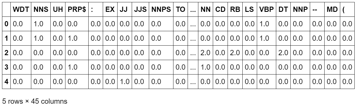
Figure 2.17: Number of occurrences of each PoS in the sentence
- To calculate the number of punctuation marks, add the following code:
def add_punctuation_count(feature_df, data):
feature_df['num_of_unique_punctuations'] = data['text'].
apply(lambda x: len(set(x).intersection
(set(punctuation))))
return feature_df
feature_df = add_punctuation_count(feature_df, data)
feature_df['num_of_unique_punctuations'].head()
The add_punctuation_count() method will find the intersection of the set of punctuation marks in the text and punctuation sets that were imported from the string module. Then, it will find the length of the intersection set in each row and add it to the num_of_unique_punctuations column of the DataFrame. The preceding code generates the following output:
0 0
1 0
2 1
3 1
4 0
Name: num_of_unique_punctuations, dtype: int64
- To calculate the number of capitalized words, add the following code:
def get_capitalized_word_count(feature_df, data):
"""
The below code line will tokenize text in every row and
create a set of only capital words, ten find the length of
this set and add it to the column 'number_of_capital_words'
of dataframe.
"""
feature_df['number_of_capital_words'] = data['text'].
apply(lambda x: len([word for word in
word_tokenize(str(x)) if word[0].isupper()]))
return feature_df
feature_df = get_capitalized_word_count(feature_df, data)
feature_df['number_of_capital_words'].head()
The preceding code will tokenize the text in every row and create a set of words consisting of only capital words. It will then find the length of this set and add it to the number_of_capital_words column of the DataFrame. The preceding code generates the following output:
0 1
1 1
2 1
3 1
4 1
Name: number_of_capital_words, dtype: int64
The last line of the preceding code will print the number_of_capital_words column, which represents the count of the number of capital letter words in each row.
- To calculate the number of lowercase words, add the following code:
def get_small_word_count(feature_df, data):
"""
The below code line will tokenize text in every row and
create a set of only small words, then find the length of
this set and add it to the column 'number_of_small_words'
of dataframe.
"""
feature_df['number_of_small_words'] = data['text'].
apply(lambda x: len([word for word in
word_tokenize(str(x)) if word[0].islower()]))
return feature_df
feature_df = get_small_word_count(feature_df, data)
feature_df['number_of_small_words'].head()
The preceding code will tokenize the text in every row and create a set of only small words, then find the length of this set and add it to the number_of_small_words column of the DataFrame. The preceding code generates the following output:
0 4
1 3
2 7
3 3
4 2
Name: number_of_small_words, dtype: int64
The last line of the preceding code will print the number_of_small_words column, which represents the number of small letter words in each row.
- To calculate the number of letters in the DataFrame, use the following code:
def get_number_of_alphabets(feature_df, data):
feature_df['number_of_alphabets'] = data['text'].
apply(lambda x: len([ch for ch in str(x)
if ch.isalpha()]))
return feature_df
feature_df = get_number_of_alphabets(feature_df, data)
feature_df['number_of_alphabets'].head()
The preceding code will break the text line into a list of characters in each row and add the count of that list to the number_of_alphabets columns. This will produce the following output:
0 19
1 18
2 28
3 14
4 13
Name: number_of_alphabets, dtype: int64
The last line of the preceding code will print the number_of_columns column, which represents the count of the number of alphabets in each row.
- To calculate the number of digits in the DataFrame, add the following code:
def get_number_of_digit_count(feature_df, data):
"""
The below code line will break the text line in a list of
digits in each row and add the count of that list into
the columns 'number_of_digits'
"""
feature_df['number_of_digits'] = data['text'].
apply(lambda x: len([ch for ch in str(x)
if ch.isdigit()]))
return feature_df
feature_df = get_number_of_digit_count(feature_df, data)
feature_df['number_of_digits'].head()
The preceding code will get the digit count from each row and add the count of that list to the number_of_digits columns. The preceding code generates the following output:
0 0
1 0
2 0
3 0
4 0
Name: number_of_digits, dtype: int64
- To calculate the number of words in the DataFrame, add the following code:
def get_number_of_words(feature_df, data):
"""
The below code line will break the text line in a list of
words in each row and add the count of that list into
the columns 'number_of_digits'
"""
feature_df['number_of_words'] = data['text'].
apply(lambda x : len(word_tokenize(str(x))))
return feature_df
feature_df = get_number_of_words(feature_df, data)
feature_df['number_of_words'].head()
The preceding code will split the text line into a list of words in each row and add the count of that list to the number_of_digits columns. We will get the following output:
0 5
1 4
2 9
3 5
4 3
Name: number_of_words, dtype: int64
- To calculate the number of whitespaces in the DataFrame, add the following code:
def get_number_of_whitespaces(feature_df, data):
"""
The below code line will generate list of white spaces
in each row and add the length of that list into
the columns 'number_of_white_spaces
"""
feature_df['number_of_white_spaces'] = data['text'].
apply(lambda x: len([ch for ch in str(x)
if ch.isspace()]))
return feature_df
feature_df = get_number_of_whitespaces(feature_df, data)
feature_df['number_of_white_spaces'].head()
The preceding code will generate a list of whitespaces in each row and add the length of that list to the number_of_white_spaces columns. The preceding code generates the following output:
0 4
1 3
2 7
3 3
4 2
Name: number_of_white_spaces, dtype: int64
- To view the full feature set we have just created, add the following code:
feature_df.head()
We will be printing the head of the final DataFrame, which means we will print five rows of all the columns. We will get the following output:

Figure 2.18: DataFrame consisting of the features we have created
With that, we have learned how to extract general features from the given text.
Note
To access the source code for this specific section, please refer to https://packt.live/3jSsLNh.
You can also run this example online at https://packt.live/3hPFmPA.
Now, let's explore how we can extract unique features.
Bag of Words (BoW)
The Bag of Words (BoW) model is one of the most popular methods for extracting features from raw texts.
In this technique, we convert each sentence into a vector. The length of this vector is equal to the number of unique words in all the documents. This is done in two steps:
- The vocabulary or dictionary of all the words is generated.
- The document is represented in terms of the presence or absence of all words.
A vocabulary or dictionary is created from all the unique possible words available in the corpus (all documents) and every single word is assigned a unique index number. In the second step, every document is represented by a list whose length is equal to the number of words in the vocabulary. The following exercise illustrates how BoW can be implemented using Python.
Exercise 2.13: Creating a Bag of Words
In this exercise, we will create a BoW representation for all the terms in a document and ascertain the 10 most frequent terms. In this exercise, we will use the CountVectorizer module from sklearn, which performs the following tasks:
- Tokenizes the collection of documents, also called a corpus
- Builds the vocabulary of unique words
- Converts a document into vectors using the previously built vocabulary
Follow these steps to implement this exercise:
- Open a Jupyter Notebook.
- Import the necessary libraries and declare a list corpus. Add the following code to implement this:
import pandas as pd
from sklearn.feature_extraction.text import CountVectorizer
- Use the CountVectorizer function to create the BoW model. Add the following code to do this:
def vectorize_text(corpus):
"""
Will return a dataframe in which every row will ,be
vector representation of a document in corpus
:param corpus: input text corpus
:return: dataframe of vectors
"""
bag_of_words_model = CountVectorizer()
"""
performs the above described three tasks on
the given data corpus.
"""
dense_vec_matrix = bag_of_words_model.
fit_transform(corpus).todense()
bag_of_word_df = pd.DataFrame(dense_vec_matrix)
bag_of_word_df.columns = sorted(bag_of_words_model.
vocabulary_)
return bag_of_word_df
corpus = ['Data Science is an overlap between Arts and Science',
'Generally, Arts graduates are right-brained and '
'Science graduates are left-brained',
'Excelling in both Arts and Science at a time '
'becomes difficult',
'Natural Language Processing is a part of Data Science']
df = vectorize_text(corpus)
df.head()
The vectorize_text method will take a document corpus as an argument and return a DataFrame in which every row will be a vector representation of a document in the corpus.
The preceding code generates the following output:
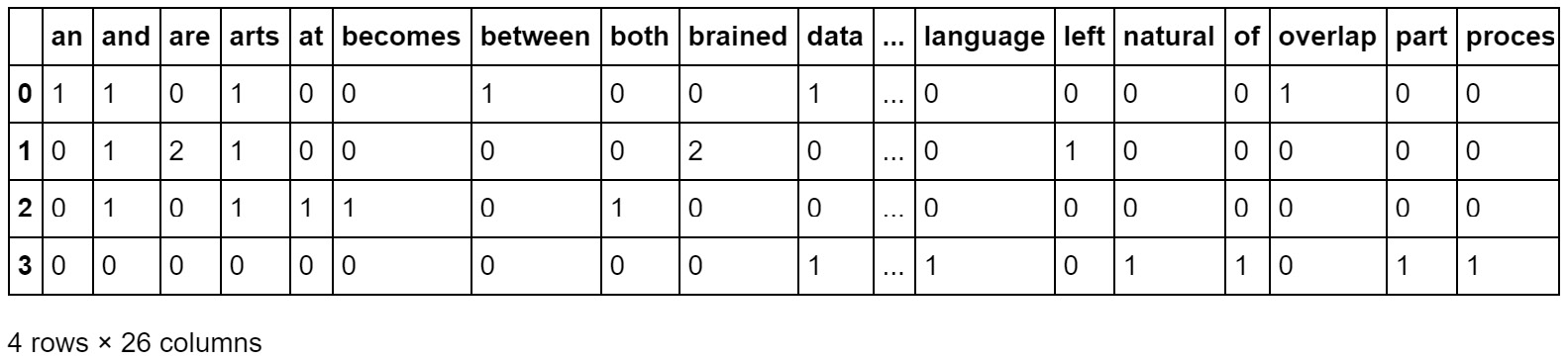
Figure 2.19: DataFrame of the output of the BoW model
- Create a BoW model for the 10 most frequent terms. Add the following code to implement this:
def bow_top_n(corpus, n):
"""
Will return a dataframe in which every row
will be represented by presence or absence of top 10 most
frequently occurring words in data corpus
:param corpus: input text corpus
:return: dataframe of vectors
"""
bag_of_words_model_small = CountVectorizer(max_features=n)
bag_of_word_df_small = pd.DataFrame
(bag_of_words_model_small.fit_transform
(corpus).todense())
bag_of_word_df_small.columns =
sorted(bag_of_words_model_small.vocabulary_)
return bag_of_word_df_small
df_2 = bow_top_n(corpus, 10)
df_2.head()
In the preceding code, we are checking the occurrence of the top 10 most frequent words in each sentence and creating a DataFrame out of it.
The preceding code generates the following output:
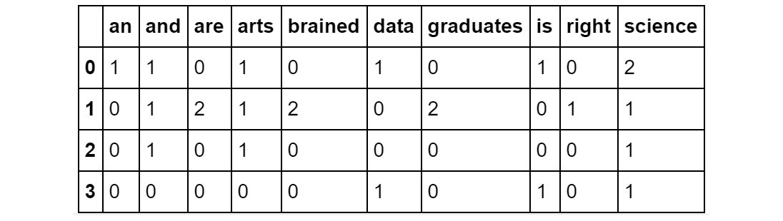
Figure 2.20: DataFrame of the output of the BoW model for the 10 most frequent terms
Note
To access the source code for this specific section, please refer to https://packt.live/3gdhViJ.
You can also run this example online at https://packt.live/3hPUTi8.
In this section, we learned what BoW is and how to can use it to convert a sentence or document into a vector. BoW is the easiest way to convert text into a vector; however, it has a severe disadvantage. This method only considers the presence and absence of words in a sentence or document—not the frequency of the words/tokens in a document. If we are going to use the semantics of any sentence, the frequency of the words plays an important role. To overcome this issue, there is another feature extraction model called TFIDF, which we will discuss later in this chapter.
Zipf's Law
According to Zipf's law, the number of times a word occurs in a corpus is inversely proportional to its rank in the frequency table. In simple terms, if the words in a corpus are arranged in descending order of their frequency of occurrence, then the frequency of the word at the ith rank will be proportional to 1/i:

Figure 2.21: Zipf's law
This also means that the frequency of the most frequent word will be twice the frequency of the second most frequent word. For example, if we look at the Brown University Standard Corpus of Present-Day American English, the word "the" is the most frequent word (its frequency is 69,971), while the word "of" is the second most frequent (with a frequency of 36,411). As we can see, its frequency is almost half of the most frequently occurring word. To get a better understanding of this, let's perform a simple exercise.
Exercise 2.14: Zipf's Law
In this exercise, we will plot both the expected and actual ranks and frequencies of tokens with the help of Zipf's law. We will be using the 20newsgroups dataset provided by the sklearn library, which is a collection of newsgroup documents. Follow these steps to implement this exercise:
- Open a Jupyter Notebook.
- Import the necessary libraries:
from pylab import *
import nltk
nltk.download('stopwords')
from sklearn.datasets import fetch_20newsgroups
from nltk import word_tokenize
from nltk.corpus import stopwords
import matplotlib.pyplot as plt
import re
import string
from collections import Counter
Add two methods for loading stop words and the data from the newsgroups_data_sample variable:
def get_stop_words():
stop_words = stopwords.words('english')
stop_words = stop_words + list(string.printable)
return stop_words
def get_and_prepare_data(stop_words):
"""
This method will load 20newsgroups data and
and remove stop words from it using given stop word list.
:param stop_words:
:return:
"""
newsgroups_data_sample =
fetch_20newsgroups(subset='train')
tokenized_corpus = [word.lower() for sentence in
newsgroups_data_sample['data']
for word in word_tokenize
(re.sub(r'([^sw]|_)+', ' ', sentence))
if word.lower() not in stop_words]
return tokenized_corpus
In the preceding code, there are two methods; get_stop_words() will load stop word list from nltk data, while get_and_prepare_data() will load the 20newsgroups data and remove stop words from it using the given stop word list.
- Add the following method to calculate the frequency of each token:
def get_frequency(corpus, n):
token_count_di = Counter(corpus)
return token_count_di.most_common(n)
The preceding method uses the Counter class to count the frequency of tokens in the corpus and then return the most common n tokens.
- Now, call all the preceding methods to calculate the frequency of the top 50 most frequent tokens:
stop_word_list = get_stop_words()
corpus = get_and_prepare_data(stop_word_list)
get_frequency(corpus, 50)
The preceding code generates the following output:
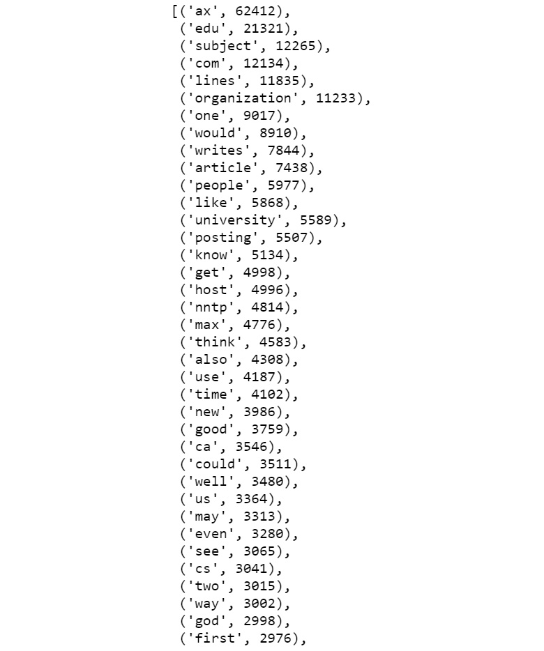
Figure 2.22: The 50 most frequent words of the corpus
- Plot the actual ranks of words that we got from frequency dictionary and the ranks expected as per Zipf's law. Calculate the frequencies of the top 10,000 words using the preceding get_frequency() method and the expected frequencies of the same list using Zipf's law. For this, create two lists—an actual_frequencies and an expected_frequencies list. Use the log of actual frequencies to downscale the numbers. After getting the actual and expected frequencies, plot them using matplotlib:
def get_actual_and_expected_frequencies(corpus):
freq_dict = get_frequency(corpus, 1000)
actual_frequencies = []
expected_frequencies = []
for rank, tup in enumerate(freq_dict):
actual_frequencies.append(log(tup[1]))
rank = 1 if rank == 0 else rank
# expected frequency 1/rank as per zipf's law
expected_frequencies.append(1 / rank)
return actual_frequencies, expected_frequencies
def plot(actual_frequencies, expected_frequencies):
plt.plot(actual_frequencies, 'g*',
expected_frequencies, 'ro')
plt.show()
# We will plot the actual and expected frequencies
actual_frequencies, expected_frequencies =
get_actual_and_expected_frequencies(corpus)
plot(actual_frequencies, expected_frequencies)
The preceding code generates the following output:
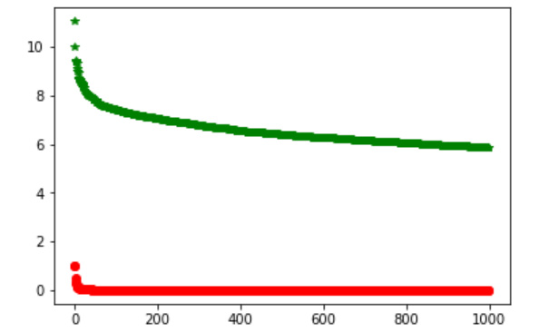
Figure 2.23: Illustration of Zipf's law
So, as we can see from the preceding output, both lines have almost the same slope. In other words, we can say that the lines (or graphs) depict the proportionality of two lists.
Note
To access the source code for this specific section, please refer to https://packt.live/30ZnKtD.
You can also run this example online at https://packt.live/3f9ZFoT.
Term Frequency–Inverse Document Frequency (TFIDF)
Term Frequency-Inverse Document Frequency (TFIDF) is another method of representing text data in a vector format. Here, once again, we'll represent each document as a list whose length is equal to the number of unique words/tokens in all documents (corpus), but the vector here not only represents the presence and absence of a word, but also the frequency of the word—both in the current document and the whole corpus.
This technique is based on the idea that the rarely occurring words are better representatives of the document than frequently occurring words. Hence, this representation gives more weightage to the rarer or less frequent words than frequently occurring words. It does so with the following formula:

Figure 2.24: TFIDF formula
Here, term frequency is the frequency of a word in the given document. Inverse document frequency can be defined as log(D/df), where df is document frequency and D is the total number of documents in the background corpus.
Now, let's complete an exercise and learn how TFIDF can be implemented in Python.
Exercise 2.15: TFIDF Representation
In this exercise, we will represent the input texts with their TFIDF vectors. We will use a sklearn module named TfidfVectorizer, which converts text into TFIDF vectors. Follow these steps to implement this exercise:
- Open a Jupyter Notebook.
- Import all the necessary libraries and create a method to calculate the TFIDF of the corpus. Add the following code to implement this:
from sklearn.feature_extraction.text import TfidfVectorizer
def get_tf_idf_vectors(corpus):
tfidf_model = TfidfVectorizer()
vector_list = tfidf_model.fit_transform(corpus).todense()
return vector_list
- To create a TFIDF model, write the following code:
corpus = ['Data Science is an overlap between Arts and Science',
'Generally, Arts graduates are right-brained and '
'Science graduates are left-brained',
'Excelling in both Arts and Science at a '
'time becomes difficult',
'Natural Language Processing is a part of Data Science']
vector_list = get_tf_idf_vectors(corpus)
print(vector_list)
In the preceding code, the get_tf_idf_vectors() method will generate TFIDF vectors from the corpus. You will then call this method on a given corpus. The preceding code generates the following output:
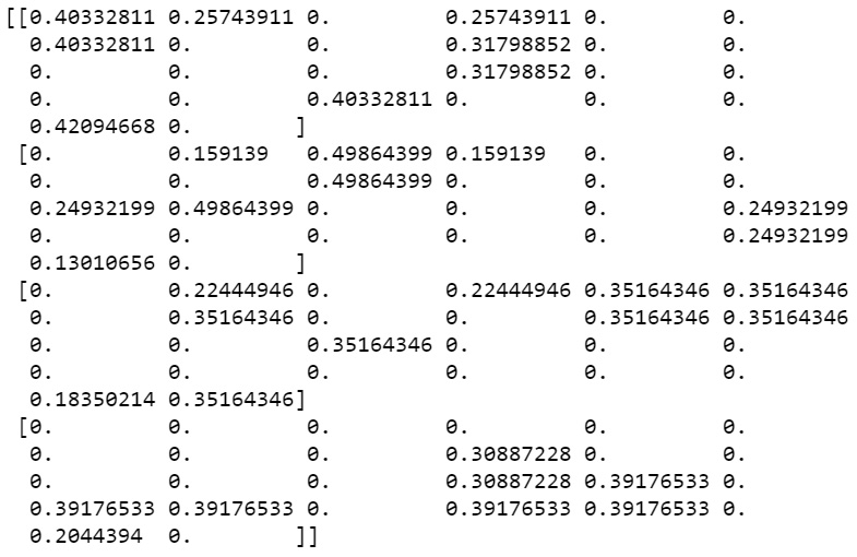
Figure 2.25: TFIDF representation of the 10 most frequent terms
The preceding output represents the TFIDF vectors for each row. As you can see from the results, each document is represented by a list whose length is equal to the unique words in the corpus and in each list (vector). The vector contains the TFIDF values of the words at their corresponding index.
Note
To access the source code for this specific section, please refer to https://packt.live/3gdzsHA.
You can also run this example online at https://packt.live/3fdP5gS.
In the next section, we will solve an activity to extract specific features from texts.
Finding Text Similarity – Application of Feature Extraction
So far in this chapter, we have learned how to generate vectors from text. These vectors are then fed to machine learning algorithms to perform various tasks. Other than using them in machine learning applications, we can also perform simple NLP tasks using these vectors. Finding the string similarity is one of them. This is a technique in which we find the similarity between two strings by converting them into vectors. The technique is mainly used in full-text searching.
There are different techniques for finding the similarity between two strings or texts. They are explained one by one here:
- Cosine similarity: The cosine similarity is a technique to find the similarity between the two vectors by calculating the cosine of the angle between them. As we know, the cosine of a zero-degree angle is 1 (meaning the cosine similarity of two identical vectors is 1), while the cosine of 180 degrees is -1 (meaning the cosine of two opposite vectors is -1). Thus, we can use this cosine angle to find the similarity between the vectors from 1 to -1. To use this technique in finding text similarity, we convert text into vectors using one of the previously discussed techniques and find the similarity between the vectors of the text. This is calculated as follows:

Figure 2.26: Cosine similarity
Here, A and B are two vectors, A.B is the dot product of two vectors, and |A| and |B| are the magnitude of two vectors.
- Jaccard similarity: This is another technique that's used to calculate the similarity between the two texts, but it only works on BoW vectors. The Jaccard similarity is calculated as the ratio of the number of terms that are common between two text documents to the total number of unique terms present in those texts.
Consider the following example. Suppose there are two texts:
Text 1: I like detective Byomkesh Bakshi.
Text 2: Byomkesh Bakshi is not a detective; he is a truth seeker.
The common terms are "Byomkesh," "Bakshi," and "detective."
The number of common terms in the texts is three.
The unique terms present in the texts are "I," "like," "is," "not," "a," "he," "is," "truth," and "seeker." So, the number of unique terms is nine.
Therefore, the Jaccard similarity is 3/9 = 0.3.
To get a better understanding of text similarity, we will complete an exercise.
Exercise 2.16: Calculating Text Similarity Using Jaccard and Cosine Similarity
In this exercise, we will calculate the Jaccard and cosine similarity for a given pair of texts. Follow these steps to complete this exercise:
- Open a Jupyter Notebook.
- Insert a new cell and add the following code to import the necessary packages:
from nltk import word_tokenize
from nltk.stem import WordNetLemmatizer
from sklearn.feature_extraction.text import TfidfVectorizer
from sklearn.metrics.pairwise import cosine_similarity
lemmatizer = WordNetLemmatizer()
- Create a function to extract the Jaccard similarity between a pair of sentences by adding the following code:
def extract_text_similarity_jaccard(text1, text2):
"""
This method will return Jaccard similarity between two texts
after lemmatizing them.
:param text1: text1
:param text2: text2
:return: similarity measure
"""
lemmatizer = WordNetLemmatizer()
words_text1 = [lemmatizer.lemmatize(word.lower())
for word in word_tokenize(text1)]
words_text2 = [lemmatizer.lemmatize(word.lower())
for word in word_tokenize(text2)]
nr = len(set(words_text1).intersection(set(words_text2)))
dr = len(set(words_text1).union(set(words_text2)))
jaccard_sim = nr / dr
return jaccard_sim
- Declare three variables named pair1, pair2, and pair3, as follows.
pair1 = ["What you do defines you", "Your deeds define you"]
pair2 = ["Once upon a time there lived a king.",
"Who is your queen?"]
pair3 = ["He is desperate", "Is he not desperate?"]
- To check the Jaccard similarity between the statements in pair1, write the following code:
extract_text_similarity_jaccard(pair1[0],pair1[1])
The preceding code generates the following output:
0.14285714285714285
- To check the Jaccard similarity between the statements in pair2, write the following code:
extract_text_similarity_jaccard(pair2[0],pair2[1])
The preceding code generates the following output:
0.0
- To check the Jaccard similarity between the statements in pair3, write the following code:
extract_text_similarity_jaccard(pair3[0],pair3[1])
The preceding code generates the following output:
0.6
- To check the cosine similarity, use the TfidfVectorizer() method to get the vectors of each text:
def get_tf_idf_vectors(corpus):
tfidf_vectorizer = TfidfVectorizer()
tfidf_results = tfidf_vectorizer.fit_transform(corpus).
todense()
return tfidf_results
- Create a corpus as a list of texts and get the TFIDF vectors of each text document. Add the following code to do this:
corpus = [pair1[0], pair1[1], pair2[0],
pair2[1], pair3[0], pair3[1]]
tf_idf_vectors = get_tf_idf_vectors(corpus)
- To check the cosine similarity between the initial two texts, write the following code:
cosine_similarity(tf_idf_vectors[0],tf_idf_vectors[1])
The preceding code generates the following output:
array([[0.3082764]])
- To check the cosine similarity between the third and fourth texts, write the following code:
cosine_similarity(tf_idf_vectors[2],tf_idf_vectors[3])
The preceding code generates the following output:
array([[0.]])
- To check the cosine similarity between the fifth and sixth texts, write the following code:
cosine_similarity(tf_idf_vectors[4],tf_idf_vectors[5])
The preceding code generates the following output:
array([[0.80368547]])
So, in this exercise, we learned how to check the similarity between texts. As you can see, the texts "He is desperate" and "Is he not desperate?" returned similarity results of 0.80 (meaning they are highly similar), whereas sentences such as "Once upon a time there lived a king." and "Who is your queen?" returned zero as their similarity measure.
Note
To access the source code for this specific section, please refer to https://packt.live/2Eyw0JC.
You can also run this example online at https://packt.live/2XbGRQ3.
Word Sense Disambiguation Using the Lesk Algorithm
The Lesk algorithm is used for resolving word sense disambiguation. Suppose we have a sentence such as "On the bank of river Ganga, there lies the scent of spirituality" and another sentence, "I'm going to withdraw some cash from the bank". Here, the same word—that is, "bank"—is used in two different contexts. For text processing results to be accurate, the context of the words needs to be considered.
In the Lesk algorithm, words with ambiguous meanings are stored in the background in synsets. The definition that is closer to the meaning of a word being used in the context of the sentence will be taken as the right definition. Let's perform a simple exercise to get a better idea of how we can implement this.
Exercise 2.17: Implementing the Lesk Algorithm Using String Similarity and Text Vectorization
In this exercise, we are going to implement the Lesk algorithm step by step using the techniques we have learned so far. We will find the meaning of the word "bank" in the sentence, "On the banks of river Ganga, there lies the scent of spirituality." We will use cosine similarity as well as Jaccard similarity here. Follow these steps to complete this exercise:
- Open a Jupyter Notebook.
- Insert a new cell and add the following code to import the necessary libraries:
import pandas as pd
from sklearn.metrics.pairwise import cosine_similarity
from nltk import word_tokenize
from sklearn.feature_extraction.text import TfidfVectorizer
from sklearn.datasets import fetch_20newsgroups
import numpy as np
- Define a method for getting the TFIDF vectors of a corpus:
def get_tf_idf_vectors(corpus):
tfidf_vectorizer = TfidfVectorizer()
tfidf_results = tfidf_vectorizer.fit_transform
(corpus).todense()
return tfidf_results
- Define a method to convert the corpus into lowercase:
def to_lower_case(corpus):
lowercase_corpus = [x.lower() for x in corpus]
return lowercase_corpus
- Define a method to find the similarity between the sentence and the possible definitions and return the definition with the highest similarity score:
def find_sentence_definition(sent_vector,defnition_vectors):
"""
This method will find cosine similarity of sentence with
the possible definitions and return the one with
highest similarity score along with the similarity score.
"""
result_dict = {}
for definition_id,def_vector in definition_vectors.items():
sim = cosine_similarity(sent_vector,def_vector)
result_dict[definition_id] = sim[0][0]
definition = sorted(result_dict.items(),
key=lambda x: x[1],
reverse=True)[0]
return definition[0],definition[1]
- Define a corpus with random sentences with the sentence and the two definitions as the top three sentences:
corpus = ["On the banks of river Ganga, there lies the scent "
"of spirituality",
"An institute where people can store extra "
"cash or money.",
"The land alongside or sloping down to a river or lake"
"What you do defines you",
"Your deeds define you",
"Once upon a time there lived a king.",
"Who is your queen?",
"He is desperate",
"Is he not desperate?"]
- Use the previously defined methods to find the definition of the word bank:
lower_case_corpus = to_lower_case(corpus)
corpus_tf_idf = get_tf_idf_vectors(lower_case_corpus)
sent_vector = corpus_tf_idf[0]
definition_vectors = {'def1':corpus_tf_idf[1],
'def2':corpus_tf_idf[2]}
definition_id, score =
find_sentence_definition(sent_vector,definition_vectors)
print("The definition of word {} is {} with similarity of {}".
format('bank',definition_id,score))
You will get the following output:
The definition of word bank is def2 with similarity of 0.14419130686278897
As we already know, def2 represents a riverbank. So, we have found the correct definition of the word here. In this exercise, we have learned how to use text vectorization and text similarity to find the right definition of ambiguous words.
Note
To access the source code for this specific section, please refer to https://packt.live/39GzJAs.
You can also run this example online at https://packt.live/3fbxQwK.
Word Clouds
Unlike numeric data, there are very few ways in which text data can be represented visually. The most popular way of visualizing text data is by using word clouds. A word cloud is a visualization of a text corpus in which the sizes of the tokens (words) represent the number of times they have occurred, as shown in the following image:
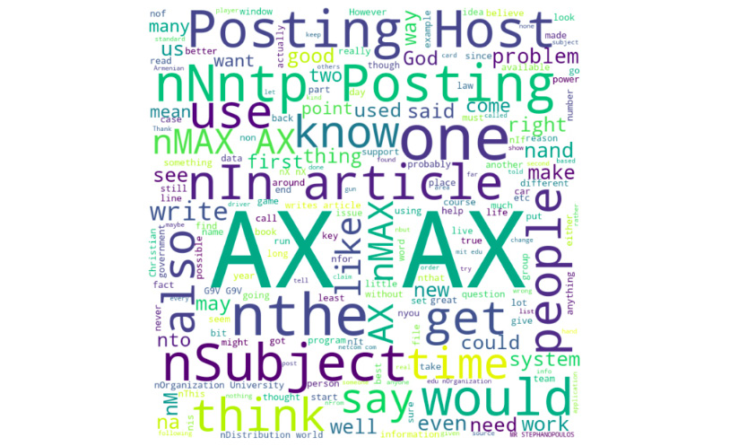
Figure 2.27: Example of a word cloud
In the following exercise, we will be using a Python library called wordcloud to build a word cloud from the 20newsgroups dataset.
Let's go through an exercise to understand this better.
Exercise 2.18: Generating Word Clouds
In this exercise, we will visualize the most frequently occurring words in the first 1,000 articles from sklearn's fetch_20newsgroups text dataset using a word cloud. Follow these steps to complete this exercise:
- Open a Jupyter Notebook.
- Import the necessary libraries and dataset. Add the following code to do this:
import nltk
nltk.download('stopwords')
import matplotlib.pyplot as plt
plt.rcParams['figure.dpi'] = 200
from sklearn.datasets import fetch_20newsgroups
from nltk.corpus import stopwords
from wordcloud import WordCloud
import matplotlib as mpl
mpl.rcParams['figure.dpi'] = 200
- Write the get_data() method to fetch the data:
def get_data(n):
newsgroups_data_sample = fetch_20newsgroups(subset='train')
text = str(newsgroups_data_sample['data'][:n])
return text
- Add a method to remove stop words:
def load_stop_words():
other_stopwords_to_remove = ['\n', 'n', '', '>',
'nLines', 'nI',"n'"]
stop_words = stopwords.words('english')
stop_words.extend(other_stopwords_to_remove)
stop_words = set(stop_words)
return stop_words
- Add the generate_word_cloud() method to generate a word cloud object:
def generate_word_cloud(text, stopwords):
"""
This method generates word cloud object
with given corpus, stop words and dimensions
"""
wordcloud = WordCloud(width = 800, height = 800,
background_color ='white',
max_words=200,
stopwords = stopwords,
min_font_size = 10).generate(text)
return wordcloud
- Get 1,000 documents from the 20newsgroup data, get the stop word list, generate a word cloud object, and finally plot the word cloud with matplotlib:
text = get_data(1000)
stop_words = load_stop_words()
wordcloud = generate_word_cloud(text, stop_words)
plt.imshow(wordcloud, interpolation='bilinear')
plt.axis("off")
plt.show()
The preceding code generates the following output:
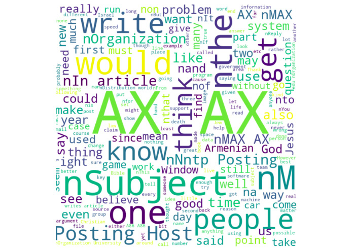
Figure 2.28: Word cloud representation of the first 10 articles
So, in this exercise, we learned what word clouds are and how to generate word clouds with Python's wordcloud library and visualize this with matplotlib.
Note
To access the source code for this specific section, please refer to https://packt.live/30eaSRn.
You can also run this example online at https://packt.live/2EzqLJJ.
In the next section, we will explore other visualizations, such as dependency parse trees and named entities.
Other Visualizations
Apart from word clouds, there are various other ways of visualizing texts. Some of the most popular ways are listed here:
- Visualizing sentences using a dependency parse tree: Generally, the phrases constituting a sentence depend on each other. We depict these dependencies by using a tree structure known as a dependency parse tree. For instance, the word "helps" in the sentence "God helps those who help themselves" depends on two other words. These words are "God" (the one who helps) and "those" (the ones who are helped).
- Visualizing named entities in a text corpus: In this case, we extract the named entities from texts and highlight them by using different colors.
Let's go through the following exercise to understand this better.
Exercise 2.19: Other Visualizations Dependency Parse Trees and Named Entities
In this exercise, we will look at two of the most popular visualization methods, after word clouds, which are dependency parse trees and using named entities. Follow these steps to complete this exercise:
- Open a Jupyter Notebook.
- Insert a new cell and add the following code to import the necessary libraries:
import spacy
from spacy import displacy
!python -m spacy download
en_core_web_sm
import en_core_web_sm
nlp = en_core_web_sm.load()
- Depict the sentence "God helps those who help themselves" using a dependency parse tree with the following code:
doc = nlp('God helps those who help themselves')
displacy.render(doc, style='dep', jupyter=True)
The preceding code generates the following output:

Figure 2.29: Dependency parse tree
- Visualize the named entities of the text corpus by adding the following code:
text = 'Once upon a time there lived a saint named '
'Ramakrishna Paramahansa. His chief disciple '
'Narendranath Dutta also known as Swami Vivekananda '
'is the founder of Ramakrishna Mission and '
'Ramakrishna Math.'
doc2 = nlp(text)
displacy.render(doc2, style='ent', jupyter=True)
The preceding code generates the following output:
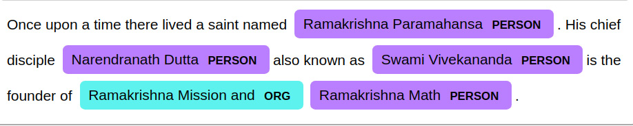
Figure 2.30: Named entities
Note
To access the source code for this specific section, please refer to https://packt.live/313m4iD.
You can also run this example online at https://packt.live/3103fgr.
Now that you have learned about visualizations, we will solve an activity based on them to gain an even better understanding.
Activity 2.02: Text Visualization
In this activity, you will create a word cloud for the 50 most frequent words in a dataset. The dataset we will use consists of random sentences that are not clean. First, we need to clean them and create a unique set of frequently occurring words.
Note
The text_corpus.txt file that's being used in this activity can be found at https://packt.live/2DiVIBj.
Follow these steps to implement this activity:
- Import the necessary libraries.
- Fetch the dataset.
- Perform the preprocessing steps, such as text cleaning, tokenization, and lemmatization, on the fetched data.
- Create a set of unique words along with their frequencies for the 50 most frequently occurring words.
- Create a word cloud for these top 50 words.
- Justify the word cloud by comparing it with the word frequency that you calculated.
Note
The solution to this activity can be found on page 375.
Summary
In this chapter, you have learned about various types of data and ways to deal with unstructured text data. Text data is usually extremely noisy and needs to be cleaned and preprocessed, which mainly consists of tokenization, stemming, lemmatization, and stop-word removal. After preprocessing, features are extracted from texts using various methods, such as BoW and TFIDF. These methods convert unstructured text data into structured numeric data. New features are created from existing features using a technique called feature engineering. In the last part of this chapter, we explored various ways of visualizing text data, such as word clouds.
In the next chapter, you will learn how to develop machine learning models to classify texts using the feature extraction methods you have learned about in this chapter. Moreover, different sampling techniques and model evaluation parameters will be introduced.