
About
This section is included to assist you in performing the activities present in the book. It includes detailed steps that are to be performed by the students to complete and achieve the objectives of the book.
1. Vital Python – Math, Strings, Conditionals, and Loops
Activity 1: Assigning Values to Variables
Solution:
- We begin with the first step, where x has been assigned the value of 14:
x = 14
- Now we use the += operator to set x equal to x + 1 in the same step:
x += 1
- In this step, x is divided by 5, and the result is squared:
(x/5) ** 2
You should get the following output:
9.0
With this activity, you have learned how to perform multiple mathematical operations on a variable. This is very common in Python. For example, in machine learning, covered in Chapter 11, Machine Learning, the input may be a matrix, X, and multiple mathematical operations will be performed on the X matrix until predictive results are obtained. Although the mathematics behind machine learning is more sophisticated, the core ideas are the same.
Activity 2: Finding a Solution Using Pythagorean Theorem in Python
Solution:
- Open your Jupyter Notebook.
- In this step, you need to write a docstring that describes the code as follows:
"""
This document determines the Pythagorean Distance
between three given points
"""
- Now, in the following code snippet, you have set x, y, and z equal to 2, 3, and 4:
# Initialize variables
x, y, z = 2, 3, 4
- In the following steps, 4 and 5, you determine the Pythagorean distance between the three points by squaring each value using the w_squared variable and taking the square root of the sum. And in the final step, you add comments to clarify each line of code:
# Pythagorean Theorem in 3 dimensions
w_squared = x**2 + y**2 + z**2
- Now, we take the square root of the sum, which will give us the distance in the final step:
# The square root gives the distance
w = w_squared ** 0.5
- To print the distance, we simply enter the w variable to output the final distance:
#Show the distance
w
You should get the following output:
5.385164807134504
In this activity, you have written a mini program that determines the Pythagorean distance between three points. Significantly, you have added a docstring and comments to clarify the code. There is never a correct answer for comments. It's up to the writer to determine how much information to give. A general goal is to be terse but informative. Comprehension is the most important thing. Adding comments and docstrings will always make your code look more professional and easier to read.
Congratulations on making it through the first topic in your Python journey! You are well on your way to becoming a developer or data scientist.
Activity 3: Using the input() Function to Rate Your Day
Solution:
- We begin this activity by opening up a new Jupyter Notebook.
- In this step, a question is displayed, prompting a user to rate their day on a number scale:
# Choose a question to ask
print('How would you rate your day on a scale of 1 to 10?')
- In this step, the user input is saved as a variable:
# Set a variable equal to input()
day_rating = input()
You should get the following output:

Figure 1.20: Output asking the user for an input value
- In this step, a statement is displayed that includes the provided number:
# Select an appropriate output.
print('You feel like a ' + day_rating + ' today. Thanks for letting me know')
You should get the following output:

Figure 1.21: Output displaying the user's day rating on a scale of 1 to 10
In this activity, you prompted the user for a number and used that number to display a statement back to the user that includes the number. Communicating directly with users depending upon their input is a core developer skill.
Activity 4: Finding the Least Common Multiple (LCM)
Solution:
- We begin by opening a new Jupyter Notebook.
- Here, you begin by setting the variables equal to 24 and 36:
# Find the Least Common Multiple of Two Divisors
first_divisor = 24
second_divisor = 36
- In this step, you have initialized a while loop based on the counting Boolean, which is True, with an iterator, i:
counting = True
i = 1
while counting:
- This step sets up a conditional to check whether the iterator divides both numbers:
if i % first_divisor == 0 and i % second_divisor == 0:
- This step breaks the while loop:
break
- This step increments the iterator at the end of the loop:
i += 1
print('The Least Common Multiple of', first_divisor, 'and', second_divisor, 'is', i, '.')
The aforementioned code snippet prints the results.
You should get the following output:
The Least Common Multiple of 24 and 36 is 72.
In this activity, you used a while loop to run a program that computes the LCM of two numbers. Using while loops to complete tasks is an essential ability for all developers.
Activity 5: Building Conversational Bots Using Python
Solution:
For the first bot, the solution is as follows:
- This step shows the first question asked of the user:
print('What is your name?')
- This step shows the response with the answer:
name = input()
print('Fascinating.', name, 'is my name too.')
You should get the following output:
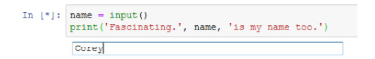
Figure 1.22: Using the input() function to ask the user to enter a value
Once you enter the value, in this case, your name, the output will be as follows:
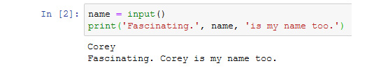
Figure 1.23: Output once the user has entered the values
- This step shows the second question asked of the user:
print('Have you thought about black holes today?')
You should get the following output:
Have you thought about black holes today?
- This step shows the response with the answer:
yes_no = input()
print('I am so glad you said', yes_no, '. I was thinking the same thing.')
You should get the following output:
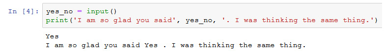
Figure 1.24: Using the input() function asks the user to enter the value
Once you enter the value, in this case, your name, the output will be as follows:
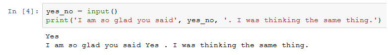
Figure 1.25: Printing the input() function statements
- This step shows the response with the answer:
print('We're kindred spirits,', name, '. Talk later.')
You should get the following output:
We're kindred spirits, Corey.Talk later.
Now, moving on to the second bot:
- Create an input() function for a smart variable and change the type to int:
print('How intelligent are you? 0 is very dumb. And 10 is a genius')
smarts = input()
smarts = int(smarts)
- Create an if loop so that if the user enters a value equal to or less than 3, we print I don't believe you. If not, then print the next statement:
if smarts <= 3:
print('I don't believe you.')
print('How bad of a day are you having? 0 is the worst, and 10 is the best.')
- Create an input() function for the day variable and change the type to int:
day = input()
day = int(day)
- Now, create an if else loop where if the user entered a value less than or equal to 5, we print the output statement. If not, then we print the output else statement:
if day <= 5:
print('If I was human, I would give you a hug.')
else:
print('Maybe I should try your approach.')
- Continue the loop using elif, also called else-if, where if the user enters a value less than or equal to 6, we print the corresponding statement:
elif smarts <= 6:
print('I think you're actually smarter.')
print('How much time do you spend online? 0 is none and 10 is 24 hours a day.')
- Now, build another input() function for the hours variable and change the type to int. Use the if-else loop so that if the user enters a value less than or equal to 4, we print the corresponding statement. If not, print the other statement:
hours = input()
hours = int(hours)
if hours <= 4:
print('That's the problem.')
else:
print('And I thought it was only me.')
- Using the elif loop, we check the smart variable and output the corresponding print statement. We also use if-else to find out whether the user has entered a value less than or equal to 5:
elif smarts <= 8:
print('Are you human by chance? Wait. Don't answer that.')
print('How human are you? 0 is not at all and 10 is human all the way.')
human = input()
human = int(human)
if human <= 5:
print('I knew it.')
else:
print('I think this courtship is over.')
- We continue with the else loop from the if-else from step 7 and set the appropriate conditions and print statements:
else:
print('I see... How many operating systems do you run?')
- Set the input() functions once again to the os variable and change the type to int, after which we output the corresponding print statement depending on the user's input values:
os = input()
os = int(os)
if os <= 2:
print('Good thing you're taking this course.')
else:
print('What is this? A competition?')
You should get the following output:
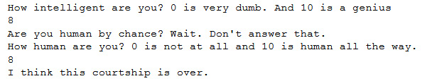
Figure 1.26: Expected outcome from one of the possible values entered by the user
Congratulations! By completing this activity, you have created two conversational bots using nested conditionals and if-else loops where we also used changing types, using the input() function to get values from the user and then respectively displaying the output.
2. Python Structures
Activity 6: Using a Nested List to Store Employee Data
Solution:
- Begin by creating a list, adding data, and assigning it to employees:
employees = [['John Mckee', 38, 'Sales'], ['Lisa Crawford', 29, 'Marketing'], ['Sujan Patel', 33, 'HR']]
print(employees)
You should get the following output:

Figure 2.31: Output when we print the content of employees
- Next, we can utilize the for..in loop to print each of the record's data within employee:
for employee in employees:
print(employee)

Figure 2.32: Output when printing each of the records inside employees
- To have the data presented in a structured version of the employee record, add the following lines of code:
for employee in employees:
print("Name:", employee[0])
print("Age:", employee[1])
print("Department:", employee[2])
print('-' * 20)
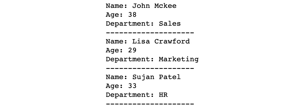
Figure 2.33: Output when printing each of the records inside employees with a structure
- Lastly, if we were to print the details of Lisa Crawford, we would need to use the indexing method. Lisa's record is in position 1, so we would write:
employee = employees[1]
print(employee)
print("Name:", employee[0])
print("Age:", employee[1])
print("Department:", employee[2])
print('-' * 20)

Figure 2.34: Output when printing the details of Lisa Crawford
Having successfully completed this activity, you will be able to work with lists and nested lists. As mentioned in the activity, this is just one instance where this concept could come in handy, that is, to store data in lists and then access them as required.
Activity 7: Storing Company Employee Table Data Using a List and a Dictionary
Solution:
- Open a Jupyter Notebook and enter the following code in it:
employees = [
{"name": "John Mckee", "age":38, "department":"Sales"},
{"name": "Lisa Crawford", "age":29, "department":"Marketing"},
{"name": "Sujan Patel", "age":33, "department":"HR"}
]
print(employees)
You should get the following output:

Figure 2.35: Output when we print the employees list
In step 1, we created a list, employee, and added values to it, such as name, age, and department.
- Now, we will be adding a for loop to our employee list using the * operator. To do this, we will use a dictionary to print the employee details in a presentable structure:
for employee in employees:
print("Name:", employee['name'])
print("Age:", employee['age'])
print("Department:", employee['department'])
print('-' * 20)
You should get the following output:

Figure 2.36: Output when we print an individual employee in a structured format
Note
You can compare this method with the previous activity, where we printed from a nested list. Using a dictionary gives us a more concise syntax, as we access the data using a key instead of a positional index. This is particularly helpful when we are dealing with objects with many keys.
- The final step is to print the employee details of Sujan Patel. To do this, we will access the employees dictionary and will only print the value of one employee from a list of employee names:
for employee in employees:
if employee['name'] == 'Sujan Patel':
print("Name:", employee['name'])
print("Age:", employee['age'])
print("Department:", employee['department'])
print('-' * 20)
You should get the following output:

Figure 2.37: Output when we only print the employee details of Sujan Patel
Having completed this activity, you are able to work with lists and dictionaries. As you have seen, lists are very useful for storing and accessing data, which very often comes in handy in the real world when handling data in Python. Using dictionaries along with lists proves to be very useful, as you have seen in this activity.
3. Executing Python – Programs, Algorithms, Functions
Activity 8: What's the Time?
Solution:
In the following, you will find the solution code to Activity 8, What's the Time?
To make it easier to understand, the code has been broken down with explanations:
current_time.py:
"""
This script returns the current system time.
"""
- Firstly, we import the datetime library, which contains a range of useful utilities for working with dates:
import datetime
- Using the datetime library, we can get the current datetime stamp, and then call the time() function in order to retrieve the time:
time = datetime.datetime.now().time()
- If the script is being executed, this if statement will be true, and, therefore, the time will be printed:
if __name__ == '__main__':
print(time)
You should get the following output:
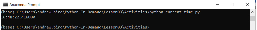
Figure 3.35: The output in the datetime format
At the end of this activity, you are able to import the datetime module and execute the Python script to tell the time. Additionally, you are able to import the time to use it elsewhere in your code if necessary.
Activity 9: Formatting Customer Names
Solution:
The customer.py file should look like the steps mentioned below. Note that there are many different valid ways to write this function:
- The format_customer function takes two required positional arguments, first_name and last_name, and one optional keyword argument, location:
def format_customer(first, last, location=None):
- It then uses the % string formatting notation to create a full_name variable:
full_name = '%s %s' % (first, last)
- The third line checks whether a location has been specified and, if so, appends the location details to the full name. If no location was specified, just the full name is returned:
if location:
return '%s (%s)' % (full_name, location)
else:
return full_name
By the end of this activity, you are able to create a function that takes in various arguments for names and returns a string as you require.
Activity 10: The Fibonacci Function with an Iteration
Solution:
- This fibonacci_iterative function starts with the first two values of the Fibonacci sequence, 0 and 1:
def fibonacci_iterative(n):
previous = 0
current = 1
- For each loop in the iteration, it updates these values to represent the previous two numbers in the sequence. After reaching the final iteration, the loop terminates, and returns the value of the current variable:
for i in range(n - 1):
current_old = current
current = previous + current
previous = current_old
return current
- Now you can try running a few examples in Jupyter Notebook by importing the fibonacci_iterative function:
from fibonacci import fibonacci_iterative
fibonacci_iterative(3)
You should get the following output:
2
Let's try another example:
fibonacci_iterative(10)
You should get the following output:
55
In this activity, you were able to work with iterations and return the nth value in the Fibonacci sequence.
Activity 11: The Fibonacci Function with Recursion
Solution:
- Open the fibonacci.py file.
- Define a fibonacci_recursive function that takes a single input named n:
def fibonacci_recursive(n):
- Now check whether the value of n is equal to 0 or 1. If the condition is satisfied, the value of n is returned. Write the following code to implement this step:
if n == 0 or n == 1:
return n
- Otherwise, in case the condition is not satisfied it will return the same function, but the argument will be decremented by 2 and 1 and the respective differences will be added:
else:
return fibonacci_recursive(n - 2) + fibonacci_recursive(n - 1)
- Once the function is created, try running the examples in the compiler using the following command:
from fibonacci import fibonacci_recursive
fibonacci_recursive(3)
You should get the following output:
2
You can now work with recursive functions. We implemented this on our fibonnacci.py file to get the expected output. Recursive functions are helpful in many cases in order to reduce the lines of code that you will be using if it is repetitive.
Activity 12: The Fibonacci Function with Dynamic Programming
Solution:
- We begin by keeping a dictionary of Fibonacci numbers in the stored variable. The keys of the dictionary represent the index of the value in the sequence (such as the first, second, and fifth number), and the value itself:
stored = {0: 0, 1: 1} # We set the first 2 terms of the Fibonacci sequence here.
- When calling the fibonacci_dynamic function, we check to see whether we have already computed the result; if so, we simply return the value from the dictionary:
def fibonacci_dynamic(n):
if n in stored:
return stored[n]
- Otherwise, we revert to the recursive logic by calling the function to compute the previous two terms:
else:
stored[n] = fibonacci_dynamic(n - 2) + fibonacci_dynamic(n - 1)
return stored[n]
- Now, run the following:
from fibonacci import fibonacci_recursive
fibonacci_dynamic(100)
You should get the following output:
354224848179261915075
In this activity, we used a function with dynamic programming that takes a single positional argument representing the number term in the sequence that we want to return.
4. Extending Python, Files, Errors, and Graphs
Activity 13: Visualizing the Titanic Dataset Using a Pie Chart and Bar Plots
Solution
- Import all the lines from the csv file in the titanic_train.csv dataset file and store it in a list:
import csv
lines = []
with open('titanic_train.csv') as csv_file:
csv_reader = csv.reader(csv_file, delimiter=',')
for line in csv_reader:
lines.append(line)
- Generate a collection of passengers objects. This step is designed to facilitate the subsequent steps where we need to extract values of different properties into a list for generating charts:
data = lines[1:]
passengers = []
headers = lines[0]
- Create a simple for loop for the d variable in data, which will store the values in a list:
for d in data:
p = {}
for i in range(0,len(headers)):
key = headers[i]
value = d[i]
p[key] = value
passengers.append(p)
- Extract the survived, pclass, age, and gender values of survived passengers into respective lists. We need to utilize list comprehension in order to extract the values; for the passengers who survived, we will need to convert survived into an integer and filter survived == 1, that is, passengers who survived:
survived = [p['Survived'] for p in passengers]
pclass = [p['Pclass'] for p in passengers]
age = [float(p['Age']) for p in passengers if p['Age'] != '']
gender_survived = [p['Sex'] for p in passengers if int(p['Survived']) == 1]
- Now, import all the necessary libraries, such as matplotlib, seaborn, and numpy, and draw a pie chart using plt.pie to visualize the passengers who survived:
import matplotlib.pyplot as plt
import seaborn as sns
import numpy as np
from collections import Counter
plt.title("Survived")
plt.pie(Counter(survived).values(), labels=Counter(survived).keys(), autopct='%1.1f%%',
colors=['lightblue', 'lightgreen', 'yellow'])
plt.show()
Execute the cell twice, and you should get the following output:
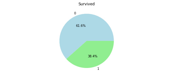
Figure 4.28: Pie chart showing the survival rate of the passengers
- Draw a column bar plot using plt.bar to visualize the passengers who survived based on their gender:
plt.title("surviving passengers count by gender")
plt.bar(Counter(gender_survived).keys(), Counter(gender_survived).values())
plt.show()
You should get the following output:
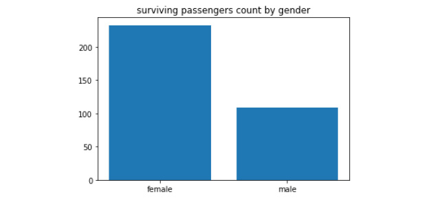
Figure 4.29: A bar plot showing the variation in gender of those who survived the incident
In this activity, we have used the interesting Titanic dataset to visualize data. We imported the dataset and stored the data in a list. Then, we used the matplotlib, seaborn, and numpy libraries to plot the various data and get the outputs as needed using the two plotting techniques: pie charts and bar plots.
5. Constructing Python – Classes and Methods
Activity 14: Creating Classes and Inheriting from a Parent Class
Solution:
- Firstly, define the parent class, Polygon. We add an init method that allows the user to specify the lengths of the sides when creating the polygon:
class Polygon():
"""A class to capture common utilities for dealing with shapes"""
def __init__(self, side_lengths):
self.side_lengths = side_lengths
def __str__(self):
return 'Polygon with %s sides' % self.num_sides
- Add two properties to the Polygon class – one that computes the number of sides of the polygon, and another that returns the perimeter:
class Polygon():
"""A class to capture common utilities for dealing with shapes"""
def __init__(self, side_lengths):
self.side_lengths = side_lengths
def __str__(self):
return 'Polygon with %s sides' % self.num_sides
@property
def num_sides(self):
return len(self.side_lengths)
@property
def perimeter(self):
return sum(self.side_lengths)
- Create a child class of Polygon called Rectangle. Add an init method that allows the user to specify the height and the width of the rectangle. Add a property that computes the area of the rectangle:
class Rectangle(Polygon):
def __init__(self, height, width):
super().__init__([height, width, height, width])
@property
def area(self):
return self.side_lengths[0] * self.side_lengths[1]
- Test your Rectangle class by creating a new rectangle and checking the value of its properties – the area and the perimeter:
r = Rectangle(1, 5)
r.area, r.perimeter
You should get the following output:
(5, 12)
- Create a child class of Rectangle called Square that takes a single height parameter in its initialization:
class Square(Rectangle):
def __init__(self, height):
super().__init__(height, height)
- Test your Square class by creating a new square and checking the value of its properties – the area and the perimeter:
s = Square(5)
s.area, s.perimeter
You should get the following output:
(25, 20)
6. The Standard Library
Activity 15: Calculating the Time Elapsed to Run a Loop
Solution:
- We begin by opening a new Jupyter file and importing the random and time modules:
import random
import time
- Then, we use the time.time function to get the start time:
start = time.time()
- Now, by using the aforementioned code, we will find the time in nanoseconds. Here, the range is set from 1 to 999:
l = [random.randint(1, 999) for _ in range(10 * 3)]
- Now, we record the finish time and subtract this time to get the delta:
end = time.time()
print(end - start)
You should get the following output:
0.0019025802612304688
- But this will give us a float. For measurements higher than 1 second, the precision might be good enough, but we can also use time.time_ns to get the time as the number of nanoseconds elapsed. This will give us a more precise result, without the limitations of floating-point numbers:
start = time.time_ns()
l = [random.randint(1, 999) for _ in range(10 * 3)]
end = time.time_ns()
print(end - start)
You should get the following output:
187500
Note
This is a good solution when using the time module and for common applications.
Activity 16: Testing Python Code
Solution:
The line, compile("1" + "+1" * 10 ** 6, "string", "exec"), will crash the interpreter; we will need to run it with the following code:
- First, import the sys and subprocess modules as we are going to use them in the following steps:
import sys
import subprocess
- We save the code that we were given in the code variable:
code = 'compile("1" + "+1" * 10 ** 6, "string", "exec")'
- Run the code by calling subprocess.run and sys.executable to get the Python interpreter we are using:
result = subprocess.run([
sys.executable,
"-c", code
])
The preceding code takes a code line, which compiles Python code that will crash and runs it in a subprocess by executing the same interpreter (retrieved via sys.executable) with the -c option to run Python code inline.
- Now, we print the final result using result.resultcode. This will return the value -11, which means the process has crashed:
print(result.returncode)
The output will be as follows:
-11
This line of code just prints the return code of the subprocess call.
In this activity, we have executed a small program that can run the requested code line and checked whether it would crash without breaking the current process. It did end up crashing, hence outputting the value -11, which corresponded to an abort in the program.
Activity 17: Using partial on class Methods
Solution:
You need to explore the functools module and realize a specific helper for methods, which can be used as explained in the following steps:
- When you execute the mentioned code, you will get the following error message:
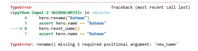
Figure 6.52: Error output with a missing required positional argument
Now, to fix this, let's check for an alternative by observing the following steps.
- Import the functools module:
import functools
- Create the Hero class, which uses partialmethod to set reset_name:
class Hero:
DEFAULT_NAME = "Superman"
def __init__(self):
self.name = Hero.DEFAULT_NAME
def rename(self, new_name):
self.name = new_name
reset_name = functools.partial(rename, DEFAULT_NAME)
def __repr__(self):
return f"Hero({self.name!r})"
The code makes use of a different version of partial, partialmethod, which allows the creation of partial for a method class. By using this utility on the rename method and setting the name to the default name, we can create partial, which will be used as a method. The name of the method is the one that is set in the scope of the Hero class definition, which is reset_name.
Wrong Assumptions with Date and Time
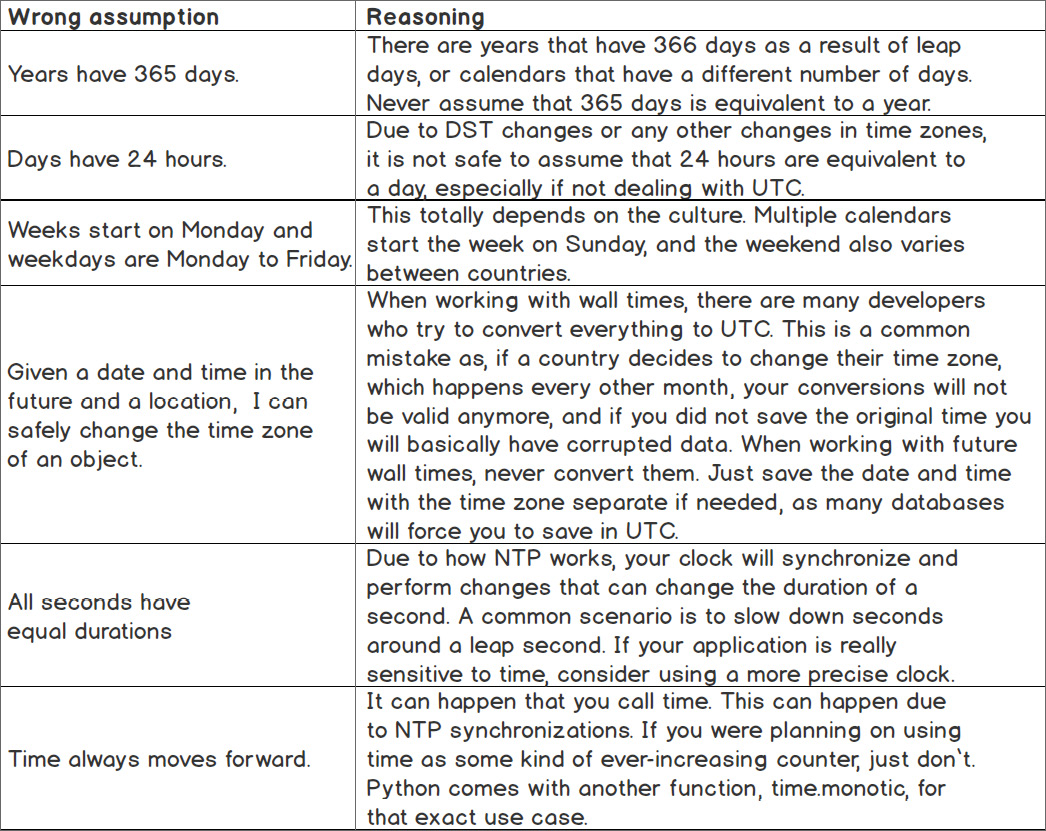
Figure 6.53: Wrong assumptions of date and time along with its reasoning
7. Becoming Pythonic
Activity 18: Building a Chess Tournament
Solution:
- Open the Jupyter Notebook.
- Define the list of player names in Python:
names = ["Magnus Carlsen", "Fabiano Caruana", "Yifan Hou", "Wenjun Ju"]
- The list comprehension uses the list of names twice because each person can either be player 1 or player 2 in a match (that is, they can play with the white or the black pieces). Because we don't want the same person to play both sides in a match, add an if clause that filters out the situation where the same name appears in both elements of the comprehension:
fixtures = [f"{p1} vs. {p2}" for p1 in names for p2 in names if p1 != p2]
- Finally, print the resulting list so that the match officials can see who will be playing whom:
print(fixtures)
You should get the following output:
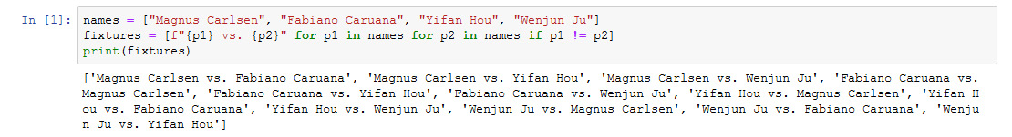
Figure 7.30: The sorted fixtures' output using a list comprehension
In this activity, we used list comprehension to sort out players and create a fixture that was in the form of a string.
Activity 19: Building a Scorecard Using Dictionary Comprehensions and Multiple Lists
Solution:
- The solution is to iterate through both collections at the same time, using an index. First, define the collections of names and their scores:
students = ["Vivian", "Rachel", "Tom", "Adrian"]
points = [70, 82, 80, 79]
Now build the dictionary. The comprehension is actually using the third collection; that is, the range of integers from 0 to 100.
- Each of these numbers can be used to index into the list of names and scores so that the correct name is associated with the correct points value:
scores = { students[i]:points[i] for i in range(4) }
- Finally, print out the dictionary you just created:
print(scores)
You should get the following output:
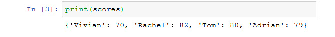
Figure 7.31: A dictionary indicating names and scores as a key-value pair
In this activity, we worked on dictionary comprehension and multiple lists. We executed the code to print out a scorecard with two separate lists of names and scores and outputted their values.
Activity 20: Using Random Numbers to Find the Value of Pi
Solution:
- You will need the math and random libraries to complete this activity:
import math
import random
- Define the approximate_pi function:
def approximate_pi():
- Set the counters to zero:
total_points = 0
within_circle = 0
- Calculate the approximation multiple times:
for i in range (10001):
Here, x and y are random numbers between 0 and 1, which, together, represent a point in the unit square (you can refer to Figure 7.25):
x = random.random()
y = random.random()
total_points += 1
- Use Pythagoras' Theorem to work out the distance between the point and the origin, (0,0):
distance = math.sqrt(x**2+y**2)
if distance < 1:
If the distance is less than 1, then this point is both inside the square and inside a circle of radius 1, centered on the origin. You can refer to Figure 7.25:
within_circle += 1
- Yield a result every 1,000 points. There's no reason why this couldn't yield a result after each point, but the early estimates will be very imprecise, so let's assume that users want to draw a large sample of random values:
if total_points % 1000 == 0:
- The ratio of points within the circle to total points generated should be approximately π/4 because the points are uniformly distributed across the square. Only some of the points are both in the square and the circle, and the ratio of areas between the circle segment and the square is π/4:
pi_estimate = 4 * within_circle / total_points
if total_points == 10000:
- After 10000 points are generated, return the estimate to complete the iteration. Using what you have learned about itertools in this chapter, you could turn this generator into an infinite sequence if you want to:
return pi_estimate
else:
Yield successive approximations to π:
yield pi_estimate
- Use the generator to find estimates for the value of π. Additionally, use a list comprehension to find the errors: the difference between the estimated version and the "actual" value in Python's math module ("actual" is in scare quotes because it too is only an approximate value). Approximate values are used because Python cannot be exactly expressed in the computer's number system without using infinite memory:
estimates = [estimate for estimate in approximate_pi()]
errors = [estimate - math.pi for estimate in estimates]
- Finally, print out our values and the errors to see how the generator performs:
print(estimates)
print(errors)
You should get the following output:
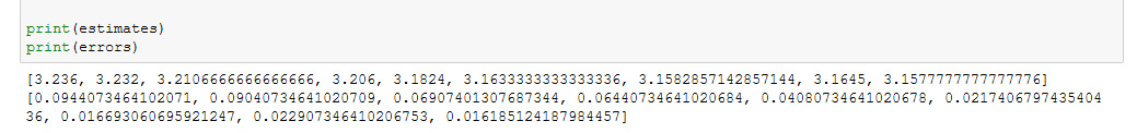
Figure 7.32: The output showing the generator yielding successive estimates of π
By completing this activity, you are now able to explain the working of generators. You successfully generated a plot of points, using which you were able to calculate the value of π. In the following section, we will learn about regular expressions.
Activity 21: Regular Expressions
Solution:
- First, create the list of names:
names = ["Xander Harris", "Jennifer Smith", "Timothy Jones", "Amy Alexandrescu", "Peter Price", "Weifung Xu"]
- Using the list comprehension syntax from this chapter makes finding the winners as easy as a single line of Python:
winners = [name for name in names if re.search("[Xx]", name)]
- Finally, print the list of winners:
print(winners)
You should get the following output:

Figure 7.33: The output showing the winners list indicating the presence of "Xx" in the customer name
In this activity, we used regular expressions and Python's re module to find customers from a list whose name contains the value of Xx.
8. Software Development
Activity 22: Debugging Sample Python Code for an Application
Solution:
- First, you need to copy the source code, as demonstrated in the following code snippet:
DEFAULT_INITIAL_BASKET = ["orange", "apple"]
def create_picnic_basket(healthy, hungry, initial_basket=DEFAULT_INITIAL_BASKET):
basket = initial_basket
if healthy:
basket.append("strawberry")
else:
basket.append("jam")
if hungry:
basket.append("sandwich")
return basket
For the first step, the code creates a list of food that is based on an initial list that can be passed as an argument. There are then some flags that control what gets added. When healthy is true, a strawberry will get added. On the other hand, if it is false, the jam will be added instead. Finally, if the hungry flag is set to true, a sandwich will be added as well.
- Run the code in your Jupyter Notebook, along with the reproducers, as demonstrated in the following code snippet:
# Reproducer
print("First basket:", create_picnic_basket(True, False))
print("Second basket:", create_picnic_basket(False, True, ["tea"]))
print("Third basket:", create_picnic_basket(True, True))
- Observe the output; the issue will show up in the third basket, where there is one extra strawberry.
You should get the following output:
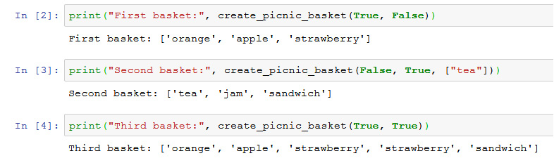
Figure 8.19: The output with the additional item in the third basket
- You will need to fix this by setting the basket value to None and using the if-else logic, as demonstrated in the following code snippet:
def create_picnic_basket(healthy, hungry, basket=None):
if basket is None:
basket = ["orange", "apple"]
if healthy:
basket.append("strawberry")
else:
basket.append("jam")
if hungry:
basket.append("sandwich")
return basket
Note that default values in functions should not be mutable, as the modifications will persist across calls. The default basket should be set to None in the function declaration, and the constant should be used within the function. This is a great exercise to debug.
- Now, run the reproducers once again, and it will be fixed.
The debugged output is as follows:
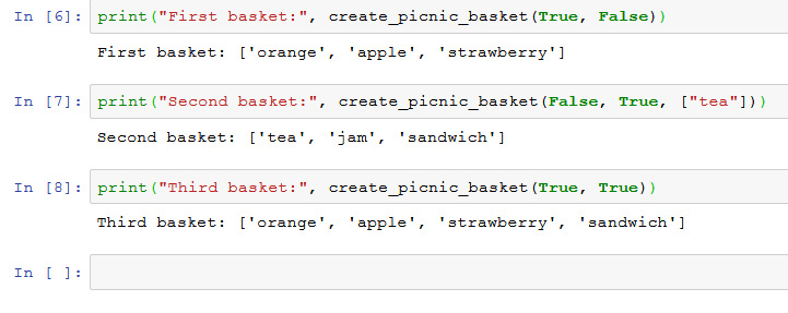
Figure 8.20: Debugging the activity with the correct output
In this activity, you have implemented debugging to understand the source code, after which you were able to print the test cases (reproducers) and find the issue. You were then able to debug the code and fix it to achieve the desired output.
9. Practical Python – Advanced Topics
Activity 23: Generating a List of Random Numbers in a Python Virtual Environment
Solution
- Create a new conda environment called my_env:
conda create -n my_env
You should get the following output:
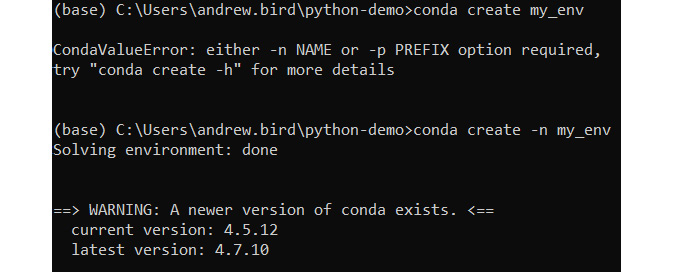
Figure 9.32: Creating a new conda environment (truncated)
- Activate the conda environment:
conda activate my_env
- Install numpy in your new environment:
conda install numpy
You should get the following output:
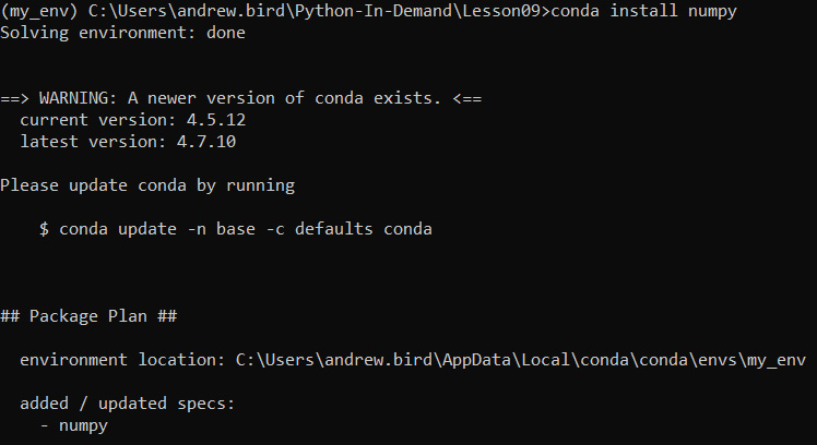
Figure 9.33: Installing numpy (truncated)
- Next, install and run a jupyter Notebook from within your virtual environment:
conda install jupyter
jupyter notebook
- Create a new jupyter Notebook and start with the following imports:
import threading
import queue
import cProfile
import itertools
import numpy as np
- Create a function that uses the numpy library to generate an array of random numbers. Recall that when threading, we need to be able to send a signal for the while statement to terminate:
in_queue = queue.Queue()
out_queue = queue.Queue()
def random_number_threading():
while True:
n = in_queue.get()
if n == 'STOP':
return
random_numbers = np.random.rand(n)
out_queue.put(random_numbers)
- Next, let's add a function that will start a thread and put integers into the in_queue object. We can optionally print the output by setting the show_output argument to True:
def generate_random_numbers(show_output, up_to):
thread = threading.Thread(target=random_number_threading)
thread.start()
for i in range(up_to):
in_queue.put(i)
random_nums = out_queue.get()
if show_output:
print(random_nums)
in_queue.put('STOP')
thread.join()
- Run the numbers on a small number of iterations to test and see the output:
generate_random_numbers(True, 10)
You should get the following output:
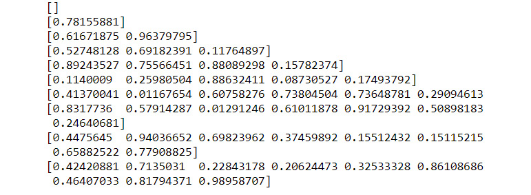
Figure 9.34: Generating lists of random numbers with numpy
- Rerun the numbers with a large number of iterations and use cProfile to view a breakdown of what is taking time to execute:
cProfile.run('generate_random_numbers(False, 20000)')
You should get the following output:
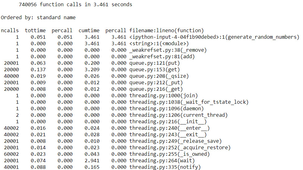
Figure 9.35: cProfile output (truncated)
Having completed this activity, you now know how to execute programs in a conda virtual environment and get the final output as a set amount of time to execute the code. You also used CProfiling to analyze the time taken by various parts of your code, giving you the opportunity to diagnose which parts of your code were the least efficient.
10. Data Analytics with pandas and NumPy
Activity 24: Data Analysis to Find the Outliers in Pay versus the Salary Report in the UK Statistics Dataset
Solution
- You begin with a new Jupyter Notebook.
- Copy the UK Statistics dataset file into a specific folder where you will be performing this activity.
- Import the necessary data visualization packages, which include pandas as pds, matplotlib as plt, and seaborn as sns:
import pandas as pd
import matplotlib.pyplot as plt
%matplotlib inline
import seaborn as sns
# Set up seaborn dark grid
sns.set()
- Choose a variable to store DataFrame and place the UKStatistics.csv file within the folder of your Jupyter Notebook. In this case, it would be as follows:
statistics_df = pd.read_csv('UKStatistics.csv')
- Now, to display the dataset, we will be calling the statistics_df variable, and .head() will show us the output of the entire dataset:
statistics_df.head()
The output will be as follows:
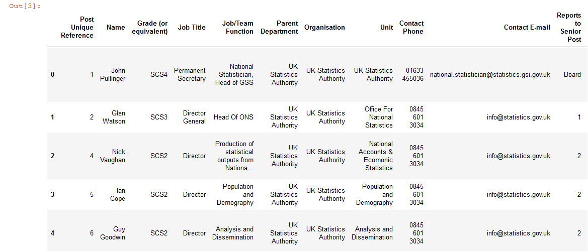
Figure 10.54: Dataset output to view
- To find the shape that is the number of rows and columns in the dataset, we use the .shape method:
statistics_df.shape
The output will be as follows:
(51, 19)
- Now, to plot a histogram of the data for Actual Pay Floor (£), we use the .hist method, as mentioned in the following code snippet. Here, you will see the difference in Pay Floor in the histogram:
plt.hist(statistics_df['Actual Pay Floor (£)'])
plt.show()
The output will be as follows:
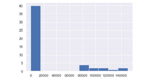
Figure 10.55: Output as a histogram
- To plot the scatter plot, we use the .scatter method, and we will be comparing the x values as Salary Cost of Reports (£), and y as Actual Pay Floor (£):
x = statistics_df['Salary Cost of Reports (£)']
y = statistics_df['Actual Pay Floor (£)']
plt.scatter(x, y)
plt.show()
The output will be as follows:
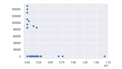
Figure 10.56: Output of the scatter plot
- Next, you need to find the difference in data, which is the data that is vastly apart from each other for x as Salary Cost of Reports (£) and y as Actual Pay Floor (£) using the box plot graph. We first assign the values of x and y, as mentioned in the following code snippet:
x = statistics_df['Salary Cost of Reports (£)']
y = statistics_df['Actual Pay Floor (£)']
- Now, to create the end outcome and check the amount of data that is closely stuck together within the box and the outliers that are presented away from the box in the graph, we use the .boxplot method to plot the graph:
plt.boxplot(x)
plt.show()
The output will be as follows:
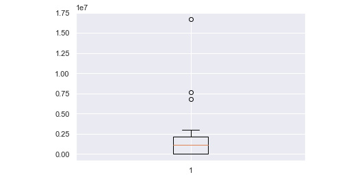
Figure 10.57: Output of the box plot
In this activity, we compared two specific pieces of data from the dataset, that is, Salary Cost of Reports (£) and Actual Pay Floor (£). We then used various graphs and observed the vast difference between Salary cost reports and Actual Pay Floor. The box plot graph clearly shows us that there are three outliers in the data of x and y that make it prone to inconsistencies with regard to pay from the government.
11. Machine Learning
Activity 25: Using Machine Learning to Predict Customer Return Rate Accuracy
Solution:
- The first step asks you to download the dataset and display the first five rows.
Import the necessary pandas and numpy libraries to begin with:
import pandas as pd
import numpy as np
- Next, load the CHURN.csv file:
df = pd.read_csv('CHURN.csv')
- Now, display the headers using .head():
df.head()
You should get the following output:
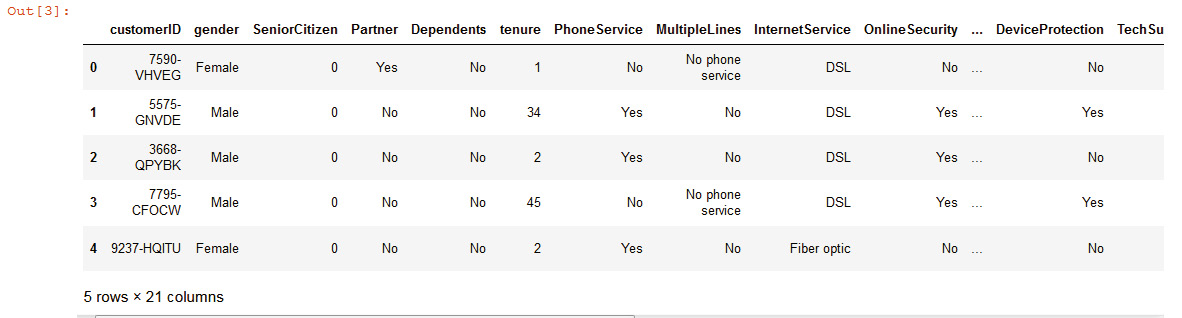
Figure 11.37: Dataset displaying the data as output
- The next step asks you to check for NaN values. The following code reveals that there are none:
df.info()
You should get the following output:
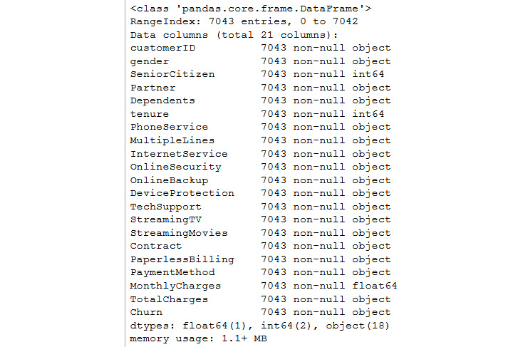
Figure 11.38: Information on the dataset
- The next step is done for you. The following code converts 'No' and 'Yes' into 0 and 1:
df['Churn'] = df['Churn'].replace(to_replace=['No', 'Yes'], value=[0, 1])
- The next step asks you to correctly define X and y. The correct solution is as follows. Note that the first column is eliminated because a customer ID would not be useful in making predictions:
X = df.iloc[:,1:-1]
y = df.iloc[:, -1]
- In order to transform all of the predictive columns into numeric columns, the following code will work:
X = pd.get_dummies(X)
- This step asks you to write a classifier function with cross_val_score. This is done as follows:
from sklearn.model_selection import cross_val_score
def clf_model (model, cv=3):
clf = model
scores = cross_val_score(clf, X, y, cv=cv)
print('Scores:', scores)
print('Mean score', scores.mean())
- The following code and output show the implementation of five classifiers, as required in this step:
By using logistic regression:
from sklearn.linear_model import LogisticRegression
clf_model(LogisticRegression())
You should get the following output:

Figure 11.39: Mean score output using LogisticRegression
By using KNeighborsClassifier:
from sklearn.neighbors import KNeighborsClassifier
clf_model(KNeighborsClassifier())
You should get the following output:

Figure 11.40: Mean score output using KNeighborsClassifier
By using GaussianNB:
from sklearn.naive_bayes import GaussianNB
clf_model(GaussianNB())
You should get the following output:

Figure 11.41: Mean score output using GaussianNB
By using RandomForestClassifier:
from sklearn.ensemble import RandomForestClassifier
clf_model(RandomForestClassifier())
You should get the following output:

Figure 11.42: Mean score output using RandomForestClassifier
By using AdaBoostClassifier:
from sklearn.ensemble import AdaBoostClassifier
clf_model(AdaBoostClassifier())
You should get the following output:

Figure 11.43: Mean score output using AdaBoostClassifier
You may or may not have the same warning as us in your notebook files. Generally speaking, warnings that do not interfere with code are okay. They are often used to warn the developer of future changes. The top three performing models, in this case, are AdaBoostClassifer, RandomForestClassifier, and Logistic Regression.
- In this step, you are asked to build a function using the confusion matrix and the classification report and run it on your top three models. The following code does just that:
from sklearn.metrics import classification_report
from sklearn.metrics import confusion_matrix
from sklearn.model_selection import train_test_split
X_train, X_test ,y_train, y_test = train_test_split(X, y, test_size = 0.25)
def confusion(model):
clf = model
clf.fit(X_train, y_train)
y_pred = clf.predict(X_test)
print('Confusion Matrix:', confusion_matrix(y_test, y_pred))
print('Classfication Report:', classification_report(y_test, y_pred))
return clf
- Now, build a function for the confusion matrix using AdaBoostClassifier:
confusion(AdaBoostClassifier())
You should get the following output:
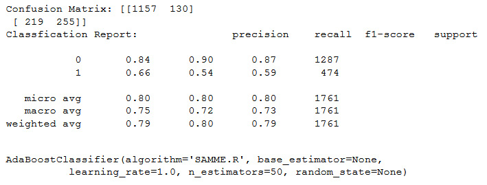
Figure 11.44: Output of the confusion matrix on AdaBoostClassifier
Confusion matrix using RandomForestClassifier:
confusion(RandomForestClassifier())
You should get the following output:
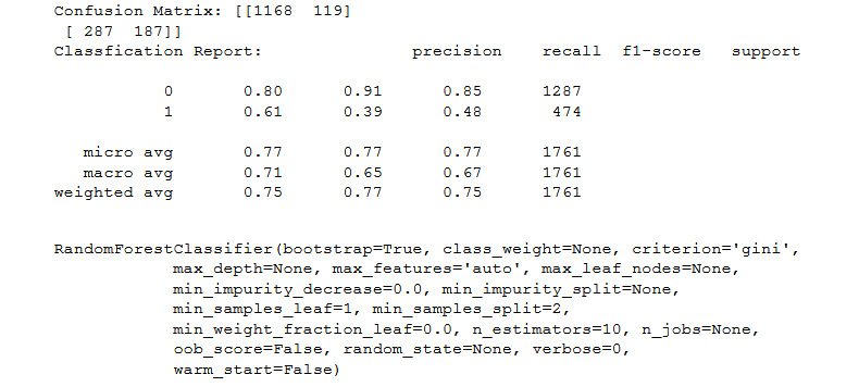
Figure 11.45: Output of the confusion matrix on RandomForestClassifier
Confusion matrix using LogisticRegression:
confusion(LogisticRegression())
You should get the following output:
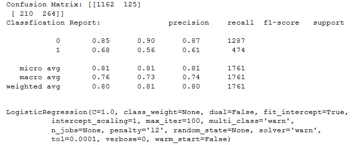
Figure 11.46: Output of the confusion matrix on LogisticRegression
- In this step, you are asked to optimize one hyperparameter for your best model. We looked up AdaBoostClassifier() and discovered the n_estimators hyperparameter, similar to the n_estimators of Random Forests. We tried several out and came up with the following result for n_estimators=250:
confusion(AdaBoostClassifier(n_estimators=250))
You should get the following output:
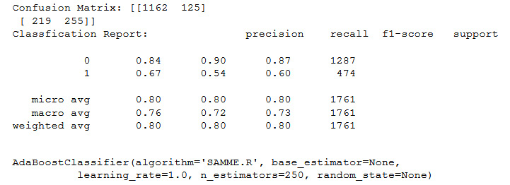
Figure 11.47: Output of the confusion matrix using n_estimators=250
- For n_estimators=25 using the AdaBoostClassifier:
confusion(AdaBoostClassifier(n_estimators=25))
You should get the following output:
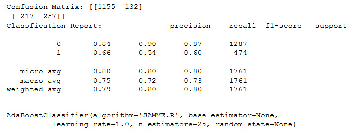
Figure 11.48: Output of the confusion matrix using n_estimators=25
- For n_estimators=15 using the AdaBoostClassifier:
confusion(AdaBoostClassifier(n_estimators=15))
You should get the following output:
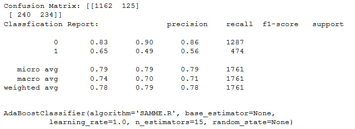
Figure 11.49: Output of the confusion matrix using n_estimators=15
As you will see by the end of this activity, when it comes to predicting user churn, AdaBoostClassifier(n_estimators = 25) gives the best predictions.