6. The Standard Library

Overview

By the end of this chapter, you will be able to utilize Python's standard library to write efficient code; use multiple standard libraries to write code; create and manipulate files by interacting with the OS filesystem; evaluate dates and times efficiently without falling into the most common mistakes and set up applications with logs to facilitate future troubleshooting.

Introduction

In the previous chapters, you saw how we can create our own classes incorporating logic and data. Yet, you often don't need to do that — you can rely on the standard library's functions and classes to do most of the work.

The Python standard library consists of modules that are available on all implementations of the language. Every installation of Python will have access to these without the need for any further steps for the modules defined in the standard library

While other famous languages don't have a standard library (such as JavaScript, which, as of 2019, is looking at implementing one), others have what seems to be an extensive set of tooling and functionality. Python goes a step further by including a vast number of basic utilities and protocol implementations as part of the default installation of the interpreter.

Standard libraries are useful and perform tasks such as unzipping files, speaking with other processes and the OS on your computer, processing HTML, and even printing graphics on the screen. A program that sorts a list of music files according to their artists can be written in a few lines when you use the correct modules of the standard library.

In this chapter, you will look at the importance of the standard library and how it can be used in our code to write faster and better Python with fewer keystrokes. You will walk through a subset of the modules, covering them in detail on a user level.

The Importance of the Standard Library

Python is often described as coming with "batteries included," which is usually a reference to its standard library. The Python standard library is vast, unlike any other language in the tech world. The Python standard library includes modules to connect to a socket; that is, one to send emails, one to connect to SQLite, one to work with the locale module, or one to encode and decode JSON and XML.

It is also renowned for including such modules as turtle and tkinter, graphical interfaces that most users probably don't use anymore, but they have proven useful when Python is taught at schools and universities.

It even includes IDLE, a Python-integrated development environment, it is not widely used as there are either other packages within the standard library that are used more often or external tools to substitute them. These libraries are divided into high-level modules and lower-level modules:

Figure 6.1: Graphical representation of the types of standard libraries

High-Level Modules

The Python standard library is truly vast and diverse, providing a toolbelt for the user that can be used to write most of their trivial programs. You can open an interpreter and run the following code snippet to print graphics on the screen. This can be executed on the Python terminal. The code mentioned here is with the >>> symbol:

>>> from turtle import Turtle, done

>>> turtle = Turtle()

>>> turtle.right(180)

>>> turtle.forward(100)

>>> turtle.right(90)

>>> turtle.forward(50)

>>> done()

This code uses the turtle module which can be used to print the output on the screen, as shown in Figure 6.2. This output will look like the trail of a turtle that follows when the cursor is moved. The turtle module allows the user to interact with the cursor and leave a trail as it keeps moving. It has functions to move around the screen and print as it advances.

Here is a detailed explanation of the turtle module code snippet:

1. It creates a turtle in the middle of the screen.
2. It then rotates it 180 degrees to the right.
3. It moves forward 100 pixels, painting as it walks.
4. It then rotates to the right once again, this time by 90 degrees.
5. It then moves forward 50 pixels once again.
6. It ends the program using done().

The code mentioned earlier in this section will result in the following output:

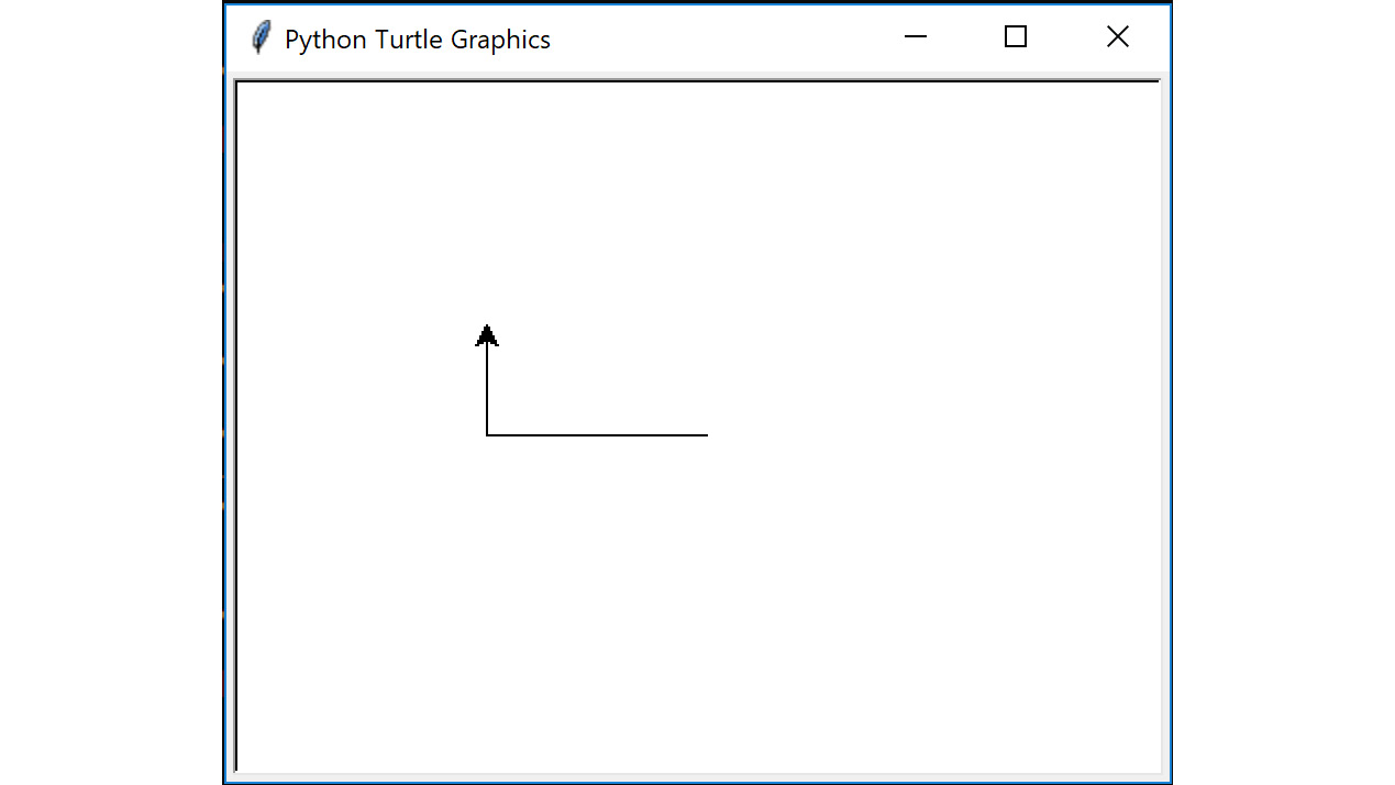
Figure 6.2: Example of output screen when using turtle

You can go ahead and explore and input different values, playing around a bit with the turtle module and checking the different outputs you get, before you dive further into this chapter.

The turtle module you worked on is an example of one of the high-level modules that the standard library offers.

Other examples of high-level modules include:

• Difflib: To check the differences line by line across two blocks of text.
• Re: For regular expressions, which will be covered in Chapter 7, Being Pythonic.
• Sqlite3: To create and interact with SQLite databases.
• Multiple data compressing and archiving modules, such as gzip, zipfile, and tarfile.
• XML, JSON, CSV, and config parser: For working with multiple file formats.
• Sched: To schedule events in the standard library.
• Argparse: For the straightforward creation of command-line interfaces.

Now, you will use another high-level module argparse as an example and see how it can be used to create a command-line interface that echoes words passed in and, optionally, capitalizes them in a few lines of code. This can be executed in the Python terminal:

>>> import argparse

>>> parser = argparse.ArgumentParser()

>>> parser.add_argument("message", help="Message to be echoed")

>>> parser.add_argument("-c", "--capitalize", action="store_true")

>>> args = parser.parse_args()

>>> if args.capitalize:

        print(args.message.capitalize())

    else:

        print(args.message)

This code example creates an instance of the ArgumentParser class, which helps you to create command-line interface applications.

It then defines two arguments in lines 3 and 4: message and capitalize.

Note that capitalize can also be referred to as -c, and we make it a Boolean flag option by changing the default action to store_true. At that point, you can just call parse_args, which will take the arguments passed in the command line, validate them, and expose them as attributes of args.

The code then takes the input message and chooses whether to capitalize it based on the flag.

You can now interact with this file, named echo.py, as shown in output Figure 6.3:

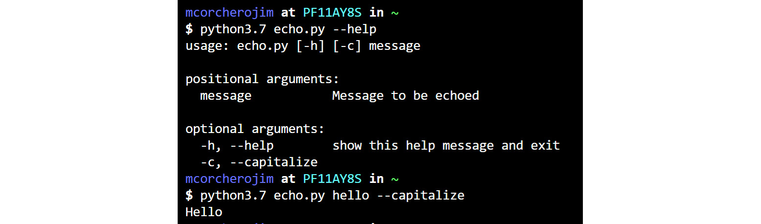
Figure 6.3: Example help message of an argparse script

Note

We will be using this capitalize tool in Exercise 86, Extending the echo.py Example.

Lower-Level Modules

The standard library also contains multiple lower-level modules that users rarely interact with. These lower-level modules are outside that of the standard library. Good examples are the different internet protocol modules, text formatting and templating, interacting with C code, testing, serving HTTP sites, and so on. The standard library comes with low-level modules to satisfy the needs of users in many of those scenarios, but you will usually see Python developers relying on libraries such as jinja2, requests, flask, cython, and cffi that are built on top of the low-level standard library module as they provide a nicer, simpler, more powerful interface. It is not that you cannot create an extension with the C API or ctypes, but cython allows you to remove a lot of the boilerplate, whereas the standard library requires you to write and optimize the most common scenarios.

Finally, there is another type of low-level module, which extends or simplifies the language. Notable examples of these are the following:

• Asyncio: To write asynchronous code
• Typing: To type hinting
• Contextvar: To save state based on the context
• Contextlib: To help with the creation of context managers
• Doctest: To verify code examples in documentation and docstrings
• Pdb and bdb: To access debugging tools

There are also modules such as dis, ast, and code that allow the developer to inspect, interact, and manipulate the Python interpreter and the runtime environment, but those aren't required by most beginner and intermediate developers.

Knowing How to Navigate in the Standard Library

Getting to know the standard library is key for any intermediate/advanced developer, even if you don't know how to use all the modules. Knowing what the library contains and when modules can be used provides any developer with a boost in speed and quality when developing Python applications.

Note

Python beginners are usually encouraged to take the standard library tour in the Python documentation (link: https://docs.python.org/3/tutorial/stdlib.html) once they master the basic syntax of the language.

While developers from other languages may try to implement everything on their own from scratch, experienced Python programmers will always first ask themselves "how can I do this with the standard library?" since using the code in the standard library brings multiple benefits, which will be explained later in the chapter.

The standard library makes code simpler and easier to understand. By using modules such as dataclasses, you can write code that would otherwise take hundreds of lines to create by ourselves and would most likely include bugs.

The dataclass module allows you to create value semantic types with fewer keystrokes by providing a decorator that can be used in a class, which will generate all the required boilerplate to have a class with the most common methods.

Note

Value semantic types represent the classes of the data that they hold. Objects can be easily copied by attributes and printed, and can then be compared using these attributes.

Exercise 85: Using the dataclass Module

In this exercise, you will create a class to hold data for a geographical point. This is a simple structure with two coordinates, x and y.

These coordinate points, x and y, are used by other developers who need to store geographical information. They will be working daily with these points, so they need to be able to create them with an easy constructor and be able to print them and see their values — converting them into a dictionary to save them into their database and share it with other people.

This exercise can be performed in the Jupyter notebook:

1. Import the dataclass module:

   import dataclasses

   This line brings the dataclasses module to the local namespace, allowing us to use it.

2. Define a dataclass:

   @dataclasses.dataclass

   class Point:

       x: int

       y: int

   With these four lines, you have defined a dataclass by its most common methods. You can now see how it behaves differently from a standard class.

3. Create an instance, which is the data for a geographical point:

   p = Point(x=10, y=20)

   print(p)

   The output will be as follows:

   Point(x=10, y=20)

4. Now, compare the data points with another Point object:

   p2 = Point(x=10, y=20)

   p == p2

   The output will be as follows:

   True

5. Serialize the data:

   dataclasses.asdict(p)

   The output will be as follows:

   {'x': 10, 'y': 20}

You now know how to use data classes to create value semantic types!

Note

Even if developers might be tempted to implement methods by themselves because they seem trivial, there are many edge cases that modules such as dataclass already takes account of, such as what happens if __eq__ receives an object of a different type or a subclass of it.

The dataclasses module is part of the standard library, so most experienced users will understand how a class decorated with a dataclass decorator will behave compared to a custom implementation of those methods. This would require either further documentation to be written, or for users to fully understand all the code in all classes that are manually crafting those methods.

Moreover, using a battle-tested code that the standard library provides is also key to writing an efficient and robust application. Functions such as sort in Python use a custom sorting algorithm known as timsort. This is a hybrid stable sorting algorithm derived from merge sort and insertion sort, and will usually result in better performance results and fewer bugs than any algorithm that a user could implement in a limited amount of time.

Exercise 86: Extending the echo.py Example

Note

In this exercise, you will be using the previously mentioned capitalize tool with help messages and a variable number of arguments.

After the creation of the capitalize tool that you saw earlier in this topic, you can implement an enhanced version of the echo tool in Linux, which is used in some embedded systems that have Python. You will, use the previous code for capitalize and enhance it to have a nicer description. This will allow the echo comman to repeat the word passed in and to take more than one word.

When you execute the code, it should generate the following help message:

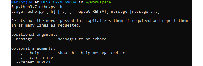
Figure 6.4: Expected output from the Exercise 86 help command

It should produce the following output when running with these arguments:

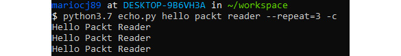
Figure 6.5: Expected output of running the Exercise 86 script

1. Add a description to the echo command.

   Start by adding a description to the echo.py script command. You can do so by passing it as an argument to the ArgumentParser class:

   parser = argparse.ArgumentParser(description="""

   Prints out the words passed in, capitalizes them if required

   and repeats them in as many lines as requested.

   """)

   The description passed in as an argument of the ArgumentParser class will be used as the help message when the user either runs the tools incorrectly or asks for help on how to use the tool.

   Note

   Notice how you can split the description into multiple lines to easily format our code, but the output appears as if all lines were together.

2. Configure an argument to take multiple messages.

   The next step is to allow multiple messages rather than a single message. You can do so by using the nargs keyword argument when adding a positional parameter:

   parser.add_argument("message", help="Messages to be echoed", nargs="+")

   By passing nargs="+", you tell argparse that we require at least one message to be passed in. Other options include ? for optional, and * for 0 or more. You can also use any natural number to require a specific number of parameters.

3. Add a repeat flag with a default value.

   Finally, you need to add a new option with a default value to control the number of times the message is repeated:

   parser.add_argument("--repeat", type=int, default=1)

   This adds a new option, repeat, which allows us to pass an integer that defaults to one, and that will control the number of times the words are repeated.

   Note

   Notice how you pass a type, which is just a callable. This will be used to transform and validate the argument passed in, and you indicate what the default value is if a user does not specify the option. Alternatively, you could have marked it as required=True to force the user to always pass a value.

   Altogether, the code and implementation will be as shown in the following code snippet:

   import argparse

   parser = argparse.ArgumentParser(description="""

   Prints out the words passed in, capitalizes them if required

   and repeat them in as many lines as requested.

   """)

   parser.add_argument("message", help="Messages to be echoed", nargs="+")

   parser.add_argument("-c", "--capitalize", action="store_true")

   parser.add_argument("--repeat", type=int, default=1)

   args = parser.parse_args()

   if args.capitalize:

       messages = [m.capitalize() for m in args.message]

   else:

       messages = args.message

   for _ in range(args.repeat):

       print(" ".join(messages))

You just created a CLI application that allows you to echo messages with an intuitive interface. You can now use the argparse module to create any other CLI application.

Quite often, the standard library in Python has answers to developers' most common questions. By having a general knowledge of the different modules in Python and always questioning what can be used from the standard library, you will write better Python code that uses easy-to-read, well-tested, and efficient utilities.

Dates and Times

Many programs will need to deal with dates and times, and Python comes with multiple modules to help you handle those effectively. The most common module is the datetime module. The datetime module comes with three types that can be used to represent dates, times, and timestamps. There are also other modules, such as the time module, or the calendar module, which can be used for some other use cases.

datetime.date can be used to represent any date between the years 1 and 9999. For any date/time outside of this range, you would need to use more specialized libraries, such as the astropy library.

You can create a datetime.date by passing the year, month, and day, or get today by just calling datetime.date.today():

import datetime

datetime.date.today()

The output is as follows:

Figure 6.6: Representation of a date object

The output format for time is similar; it takes hour, minute, second, and microsecond. All of them are optional and are initialized at 0 if not provided. This can also be created with tzinfo, but you will see more about that attribute in the datetime.datetime section.

Within the datetime module, you have what is probably the most frequently used class, the datetime.datetime class. It can represent a combination of a date and a time, and it actually inherits from datetime.date. But before you start to explore the datetime class within the datetime module, you need to better understand the concept of time and how you represent it.

There are usually two kinds of time that you need to represent. They are commonly referred to as timestamps and wall time.

The first, timestamps, can be seen as a unique point in time independent from any human interpretation of it. It is an absolute point in the line of time that is not relative to any geographical location or country. This is used for astronomical events, log records, and the synchronization of machines, among other things.

The second, wall time, refers to the time on the wall at a specific location. This is the time humans use, and you synchronize your time using it. This time is the "legal" time as it is dictated by the country and is related to a time zone. This is used for meetings, flight schedules, working hours, and so on. The interval of time can change at any point due to legislation. As an example, think of countries that observe daylight saving time (DST) and change their standard clock accordingly.

Note

If you need to work extensively with time, it is important to read about UTC and the history of how you measure time to avoid more complex issues, but you will go through a quick overview of good practices when handling time in this topic to avoid the most common mistakes.

When you are working with wall time, you just need to treat datetime.datetime objects as a mere combination of a date and a time at a location. But you should usually attach a time zone to it to be more precise and get proper semantics for time comparison and basic arithmetic. The two most commonly used libraries to handle time zones are pytz and dateutil.

You must use dateutil when using wall times; pytz has a time model that will lead the inexperienced user to make mistakes more often than not. To create a datetime with a time zone, you just need to pass it through the tzinfo argument:

import datetime

from dateutil import tz

datetime.datetime(1989, 4, 24, 10, 11,

                      tzinfo=tz.gettz("Europe/Madrid"))

This creates a datetime with that time zone information attached.

Exercise 87: Comparing datetime across Time Zones

The goal of this exercise is to create two different datetime and compare them when they are in different time zones:

1. Import the datetime and tz modules from dateutil:

   import datetime

   from dateutil import tz

   Note

   Dateutil is not a module from the standard library, though it is the one recommended by the standard library.

2. Create the first datetime for Madrid:

   d1 = datetime.datetime(1989, 4, 24, hour=11,

                            tzinfo=tz.gettz("Europe/Madrid"))

   With this line, you create a datetime for April 24, 1989, at 11 a.m. in Madrid.

3. Create the second datetime for Los_Angeles:

   d2 = datetime.datetime(1989, 4, 24, hour=8,

                            tzinfo=tz.gettz("America/Los_Angeles"))

   This creates a datetime object that seems to have a difference of 3 hours less and a different time zone.

4. Now, compare them:

   print(d1.hour > d2.hour)

   print(d1 > d2)

   The output is as follows:

   

   Figure 6.7: Output when comparing the conditions for the time zones

   When you compare the two datetime objects, you can see that even though the first datetime has a higher hour than the second (that is, the first is at 11 and the second is at 8), the first is not greater, and is, therefore later than the second, as the time zone is different, and 8 in Los Angeles happens after 11 in Madrid.

5. Now, convert the datetime object to a different time zone.

   You can convert a datetime from one time zone to another. You should do that to see what time the second datetime would show if it was in Madrid:

   d2_madrid = d2.astimezone(tz.gettz("Europe/Madrid"))

   print(d2_madrid.hour)

   The output is as follows:

   17

It is 5 p.m. Now, it is obvious that the second datetime is later than the first.

At other times, you might work just with timestamps, with time not related to any location. The easiest way to do this is to use UTC, with 0 as the offset. UTC is Coordinated Universal Time and is a system that provides a universal way of coordinating time across locations — you have most likely already used it. It is the most common standard for the time. The time zones you saw in the previous exercises define offsets from UTC that allow the library to identify what time corresponds to time from one location to another.

To create a datetime with an offset of 0, also known as a datetime in UTC, you can use datetime.timezone.utc as the tzinfo argument. This will then represent an absolute point in the line of time. You can safely add, subtract, and compare datetimes without any issue when using UTC. On the other hand, if you use any specific time zone, you should be aware that nations might change the time at any point, which could make any of your calculations invalid.

You now know how to create datetimes, compare them, and convert them across time zones. This is a common exercise when developing applications that deal with time.

In the next exercise, you'll look at the time delta between two datetime objects. Here, the delta is the difference.

Exercise 88: Calculating the Time Delta between Two datetime Objects

In this exercise, you will subtract two datetime objects to calculate the delta between the two timestamps.

Quite often, when you work with datetime, what really matters is the difference between them; that is, the delta in time between two specific dates. Here, you will find out the difference in seconds between two important events that happened in your company, one on February 25, 2019, at 10:50, and the other on February 26 at 11:20. Both these times are in UTC. This exercise can be performed in a Jupyter notebook:

1. Import the datetime module:

   import datetime as dt

   Quite often, developers import the datetime module through an alias, dt. This is done in many codebases to differentiate the datetime module from the datetime class.

2. Create two datetime objects.

   You now create two dates:

   d1 = dt.datetime(2019, 2, 25, 10, 50,

                    tzinfo=dt.timezone.utc)

   d2 = dt.datetime(2019, 2, 26, 11, 20,

                    tzinfo=dt.timezone.utc)

   We created two datetime objects as dt.datetime, and you now have two datetime objects.

3. Subtract d1 from d2.

   You can subtract two datetime to get a time delta back or add a time delta to a datetime.

   Adding two datetime makes no sense, and the operation will, therefore, output an error with an exception. Hence, you subtract the two datetime to get the delta:

   d2 – d1

   The output is as follows:

   

   Figure 6.8: Output with the delta between 2 days and seconds

4. You can see that the delta between the two datetime is 1 day and 1,800 seconds, which can be translated to the total number of seconds by calling total_seconds in the time delta object that the subtraction returns:

   td = d2 - d1

   td.total_seconds()

   The output is as follows:

   88200.0

5. It happens quite often that you need to send datetime objects in formats such as JSON or others that do not support native datetimes. A common way to serialize datetime is by encoding them in a string using the ISO 8601 standard.

   This can be done by using isoformat, which will output a string, and parsing them with the fromisoformat method, which takes a datetime serialized to a string with isoformat and transforms it back to a datetime:

   d1 = dt.datetime.now(dt.timezone.utc)

   d1.isoformat()

   The output is as follows:

Figure 6.9: Output with the datetime serialized to a string with isoformat and back to datetime

Another module that you use when dealing with time is the time module. In the time module, you can get the Unix time through time.time. This will return the number of seconds since the Unix epoch is without leap seconds. This is known as Unix time or POXIS time.

You are encouraged to read about leap seconds if you need to develop highly time-sensitive applications, but Python offers no time support for them. The time and datetime modules just use the system clock, which will not count leap seconds.

But what happens in an instance where a leap second occurs is up to the OS admin. Some companies slow down time around leap seconds, while others just skip them by making a second take two seconds in the real world. If you need to figure this out in your workplace, you will need to check with your OS admin how the NTP servers are configured to act in leap seconds. Luckily, you know well in advance when the next leap second will happen, as the International Earth Rotation and Reference Systems Service (https://packt.live/2oKYtUR) publishes leap seconds at least 8 weeks in advance.

You now understand the basics of time arithmetic and know how to calculate the time delta between two timestamps.

Exercise 89: Calculating the Unix Epoch Time

In this exercise, you will use the datetime and time modules to calculate Unix Epoch time.

If you can just look it up, you can also calculate the Unix epoch. As time.time gives us the number of seconds since the epoch, you can create a time delta with it and subtract it from a datetime you've created. You will see how to perform that in this exercise.

This exercise can be performed in a Jupyter notebook:

1. Import the time and datetime modules and get them to the current namespace:

   import datetime as dt

   import time

2. Get the current time. You use both datetime and time to do this:

   time_now = time.time()

   datetime_now = dt.datetime.now(dt.timezone.utc)

   Note

   You use the UTC time zone when getting time with datetime. This is necessary because time.time returns Unix time, which uses an epoch that is in UTC.

3. You can now calculate the epoch by subtracting datetime and a time delta, which you get from the current time since you said that these are the number of seconds since the epoch:

   epoch = datetime_now - dt.timedelta(seconds=time_now)

   print(epoch)

   The output is as follows:

Figure 6.10: Calculating the epoch

The result is the Unix epoch — January 1, 1970.

Having completed this exercise, you know how to use the time and datetime modules to get the output as the Unix epoch time, as shown in Figure 6.10, and to use timedelta to represent intervals.

There is one more module that it is sometimes used in combination with datetime, which is the calendar module. The calendar module provides additional information about calendar years; that is, how many days there are in a month. This can also be used to output calendars such as the Unix function.

Now have a look at an example where you create a calendar and get all of the days in a month as follows:

import calendar

c = calendar.Calendar()

list(c.itermonthdates(2019, 2))

The output is as follows:

Figure 6.11: Output showing month 1 and its days as a calendar

Note

Though the function returns all date instances for all the weeks in the month, if you want to get only the days that belong to the specific month, you need to filter them.

list(d for d in c.itermonthdates(2019, 2)

        if d.month == 2)

You should get the following output:

Figure 6.12: Output showing month 2 and it's days as a calendar

Note

Bear in mind in mind that when working with datetimes, there are some basic assumptions that you might make that will cause bugs in your code. For instance, assuming a year will have 365 days will cause problems for 29 February, or assuming that a day has 24 hours when any international traveler can tell you that this isn't the case. A detailed table on the wrong assumptions of time and its reasoning is mentioned in the appendix of this book on Page 541.

If you need to work with dates and times, make sure to always use well-tested libraries such as dateutil from the standard library, and consider using a good testing library such as freezegun to validate your assumptions. You'd be surprised to discover the endless number of bugs that computer systems have when exposed to time quirks.

To know more about time, you first need to understand how the system clock works. For example, your computer clock is not like a clock on the wall; it uses the Network Time Protocol (NTP) to coordinate with other connected computers. NTP is one of the oldest internet protocols that is still in use. Time is really hard to measure, and the most efficient way to do so is by using atomic clocks. The NTP creates a hierarchy of clocks and synchronizes them periodically. A good exercise is to disable the NTP sync on your computer for a day and check how your system clock deviates from the internet by running the NTP manually.

Handling dates and times properly is extremely difficult. For simple applications, you should be fine with a basic level of understanding, but otherwise, further reading and more specialized libraries will be needed. In Python, we have the datetime module as the key to handling date and time, which also contains the timezone.utc time zone. There are also time and calendar modules, which can be used when we need to measure with UNIX time and to get calendar information, respectively.

Activity 15: Calculating the Time Elapsed to Run a Loop

You are part of an IT department, and you are asked to inspect an application that outputs random numbers but with a delay. In order to investigate this delayed output, you check the code as there have been updates to the application where the development team has added a new line of code to get a list of random numbers. You are asked to confirm this by checking the time it takes to run that line of code using the time module.

Note

To perform this activity, you can just record the time by using time.time to compute the difference in time since, before, and after the function. If you want to be more precise and use the time in nanoseconds, you can use time_ns.

You will see in the topic about profiling in a later chapter how to measure performance in a more precise way.

This was the line of code that was added in by the development team:

l = [random.randint(1, 999) for _ in range(10 * 3)]

While it is possible to run the code and use time.time to calculate the elapsed time, is there any better function in the time module to do this?

Steps:

1. Record the time before running the code mentioned above in a hint with the time.time function.
2. Record the time after running the code mentioned above in a hint with the time.time function.
3. Find the difference between the two.
4. Repeat the steps using time.time_ns.

   You should get the following output:

   187500

   Note

   The solution for this activity is available on page 538.

Interacting with the OS

One of the most common uses of Python is to write code that interacts with the OS and its filesystem. Whether you are working with files or you just need some basic information about the OS, this topic will cover the essentials of how to do it in a multiplatform way through the os, sys, platform, and pathlib modules of the standard library.

OS Information

There are three key modules that are used to inspect the runtime environment and the OS. The os module enables miscellaneous interfaces with the OS. You can use it to inspect environment variables or to get other user and process-related information. This, combined with the platform module, which contains information about the interpreter and the machine where the process is running, and the sys module, which provides you with helpful system-specific information, will usually provide you with all the information that you need about the runtime environment.

Exercise 90: Inspecting the Current Process Information

The goal of this exercise is to use the standard library to report information about the running process and the platform on your system:

1. Import the os, platform, and sys modules:

   import platform

   import os

   import sys

2. Get basic process information:

   To obtain information such as the Process id, Parent id you can use the os module:

   print("Process id:", os.getpid())

   print("Parent process id:", os.getppid())

   The output is as follows:

   

   Figure 6.13: The expected output showing the process ID and the parent process ID of the system

   This gives us the process ID and the parent process ID. This constitutes a basic step when you try to perform any interaction with the OS that involves your process and is the best way to uniquely identify the running process. You can try restarting the kernel or the interpreter and see how the pid changes, as a new process ID is always assigned to a running process in the system.

3. Now, get the platform and Python interpreter information:

   print("Machine network name:", platform.node())

   print("Python version:", platform.python_version())

   print("System:", platform.system())

   The output is as follows:

   

   Figure 6.14: The expected output showing the network name, Python version, and the system type

   These functions of the module platform can be used to ascertain the information of the computer where your Python code is running, which is useful when you are writing code that might be specific to the machine or system information.

4. Get the Python path and the arguments passed to the interpreter:

   print("Python module lookup path:", sys.path)

   print("Command to run Python:", sys.argv)

   This will give us a list of paths where Python will look for modules and the command line that was used to start the interpreter as a list of arguments.

5. Get the username through an environment variable.

   print("USERNAME environment variable:", os.environ["USERNAME"])

   The output is as follows:

Figure 6.15: The expected output showing the username environment variable

The environ attribute of the os module is a dict that maps the environment variable name to its values. The keys are the name of the environment variables, and the value is the one that it was set to initially. It can be used to read and set environment variables, and it has the methods that you would expect a dict. You can use os.environ.get(varname, default) to provide a default value if a variable was not set, and pop to remove items or just assign a new value. There are also two other methods, getenv and putenv, which can be used to get and set environment variables, but, using the os.environ as a dict is more readable.

This is just a small peek into these three modules and some of the attributes and functions that they provide. Further and more specialized information can be found in the modules, and you are encouraged to explore the module when any specific runtime information is needed.

Having completed this exercise, you learned how to use multiple modules such as os and platform to query information about the environment that can be used to create programs that interact with it.

Using pathlib

Another useful module is pathlib. Even though many of the actions that are performed with pathlib can be done with os.path, the pathlib library offers a much better experience, which you'll go into more detail about later.

The pathlib module provides a way to represent and interact with filesystem paths.

A path object of the module, which is the basic util of the module, can just be created with its default argument to start a relative path to the current working directory:

import pathlib

path = pathlib.Path()

print(repr(path))

You should get the following output:

WindowsPath('.')

Note

You can get and change the current working directory with os.getcwd() and os.chdir(), respectively.

You will get either a PosixPath or a WindowsPath function of the platform you are running on.

You can use the string representation of a path at any time to be used in the functions that accept a string as a path; this can be done by calling str(path).

path objects can be joined with just a forward slash (/), which feels really natural and easy to read, as shown in the following code snippet:

import pathlib

path = pathlib.Path(".")

new_path = path / "folder" / "folder" / "example.py"

You can now perform multiple operations on those path objects. One of the most common ones is to call resolve in the resulting object, which will make the path absolute and resolve all .. references. As an example, paths such as ./my_path/ will be resolved to paths such as /current/workspace/my_path, which start with the root filesystem.

Some of the most common operations to perform on a path are the following:

• exists: Checks whether the path exists in the filesystem and whether it is a file or a directory.
• is_dir: Checks whether the path is a directory.
• is_file: Checks whether the path is a file.
• iterdir: Returns an iterator with path objects to all the files and directories contained within the path object.
• mkdir: Creates a directory in the path indicated by the path object.
• open: Opens a file in the current path, similar to running open and passing the string representation of the path. It returns a file object that can be operated like any other.
• read_text: Returns the content of the file as a Unicode string. If the file is in binary format, the read_bytes method should be used instead.

Finally, a key function of Path objects is glob. Glob allows you to specify a set of filenames by using wildcards. The main character used to do so is *, which matches any character in the path level. ** matches any name but crossing directories. This means that "/path/*" will match any file in "path" whilst "/path/**" and will match any file within its path and any of its directories.

You will look at this in the next exercise.

Exercise 91: Using the glob Pattern to List Files within a Directory

In this exercise, you will learn how to list the files of an existing source tree. This is a key part of developing any application that works with a filesystem.

You are given the following file and folder structure, which you have in the GitHub repository:

Figure 6.16: Initial folder structure

1. Create a path object for the current path:

   import pathlib

   p = pathlib.Path("")

   Note

   You could also use pathlib.Path.cwd() and get an absolute path directly.

2. Find all files in the directory with the txt extension.

   You can start by listing all files with the txt extension by using the following glob:

   txt_files = p.glob("*.txt")

   print("*.txt:", list(txt_files))

   The output is as follows:

   

   Figure 6.17: Output showing the file with the .txt extension

   This lists all the files in the current location that end with txt, which, in this case, is the only file_a.txt. Folders within other directories are not listed, as the single star, *, does not cross directories and if there was another file not ending in txt, it would not be included either.

   Note how you need to transform txt_files into a list. This is needed as glob returns an iterator and you want to print the list. This is useful since, when you are listing files, there might be an endless number of files.

   If you wanted to list all of the text files in any folder within the path, no matter the number of subdirectories, you could use the double star syntax, **:

   print("**/*.txt:", list(p.glob("**/*.txt")))

   The output is as follows:

   

   Figure 6.18: Output showing all the files in all the folders

   This lists all files that end with .txt within any folder in the current path described by the path object, p.

   This lists folder_1/file_b.txt and folder_2/folder_3/file_d.txt, but also file_a.txt, which is not within any folder, as ** matches within any number of nested folders, including 0.

   Note

   folder_1/file_c.py won't be listed, however, as it does not match the ending we provided in the glob.

3. List all files one level deep that are within the subdirectory.

   If you wanted to list all files one level deep within a subdirectory only, you could use the following glob pattern:

   print("*/*:", list(p.glob("*/*")))

   The output is as follows:

Figure 6.19: Output showing the files within a subdirectory

This will list both files within folder_1 and the folder "folder_2/folder_3, which is also a path. If you wanted to get only files, you could filter each of the paths by checking the is_file method, as mentioned previously:

print("Files in */*:", [f for f in p.glob("*/*") if f.is_file()])

The output is as follows:

Figure 6.20: Output showing the files within folder_1, folder_2, and folder_3

This will not include paths that are no longer a file.

Note

There is also another module that is worth mentioning, which contains high-level functions for file and folder operations, shutil. With shutil, it is possible to recursively copy, move, or delete files.

You now know how to list files within a tree based on their attributes or extensions.

Listing All Hidden Files in Your Home Directory

In Unix, hidden files are those that start with a dot. Usually, those files are not listed when you list files with tools such as ls unless you explicitly ask for them. You will now use the pathlib module to list all hidden files in your home directory. The code snippet indicated here will show exactly how to list these hidden files:

import pathlib

p = pathlib.Path.home()

print(list(p.glob(".*")))

The pathlib docs find the function that gives us the home directory, and then we use the glob pattern to match any file starting with a dot. In the next topic, we will be using the subprocess module.

Using the subprocess Module

Python is really useful in situations where we need to start and communicate with other programs on the OS.

The subprocess module allows us to start a new process and communicate with it, bringing to Python all the available tools installed on your OS through an easy-to-use API. The subprocess module can be seen by calling any other program from your shell.

This module has gone through some work to modernize and simplify its API, and you might see code using subprocess in ways different from those shown in this topic.

The subprocess module has two main APIs: the subprocess.run call, which manages everything from you passing the right arguments; and subprocess.Popen, a lower-level API that is available for more advanced use cases. You are going to cover only the high-level API, subprocess.run, but if you need to write an application that requires something more complex, as we have previously seen with the standard library, go through the documentation and explore the APIs for more complex use cases.

Note

The following examples have been run on a Linux system, but subprocess can be used on Windows as well; it will just need to call Windows programs. You can use dir instead of ls, for example.

Now you will see how you can call the Linux system ls by using subprocess and listing all the files:

import subprocess

subprocess.run(["ls"])

This will just create a process and run the ls command. If the ls command is not found (in Windows, for example), running this command will fail and raise an exception.

Note

The return value is an instance of CompletedProcess, but the output of the command is sent to standard output in the console.

If you want to be able to capture and see the output that our process produced, you need to pass the capture_output argument. This will capture stdout and stderr and make it available in the completedProcess instance returned by run:

result = subprocess .run(["ls"], capture_output=True)

print("stdout: ", result.stdout)

print("stderr: ", result.stderr)

The output is as follows:

Figure 6.21: Output showing the subprocess module

Note

The stdout and stderr result is a byte string. If you know that the result is text, you can pass the text argument to have it decoded.

Now, Let's omit stderr from the output as you know it is empty as shown in the Figure 6.21.

result = subprocess .run(        ["ls"],

        capture_output=True, text=True

    )

print("stdout: ", result.stdout)

The output is as follows:

Figure 6.22: Output showing the subprocesses using stdout

You can also pass more arguments, such as -l, to have the files listed with details:

result = subprocess.run(        ["ls", "-l"],

        capture_output=True, text=True

    )

print("stdout: ", result.stdout)

The output is as follows:

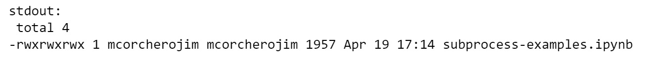
Figure 6.23: Output showing the files listed in detail using -l

The first thing that usually surprises users when using suprocess.run is that the command that needs to be passed in to run is a list of strings. This is for convenience and security. Many users will jump into using the shell argument, which will make passing the command arguments as a string work but there are security concerns. When doing so, you are basically asking Python to run our command in the system shell, and you are therefore responsible for escaping the characters as needed. Imagine for a moment that you accept user input, and you are going to pass it to the echo command. A user would then be able to pass hacked; rm –rf / as the argument for echo.

Note

Do not run this command: hacked; rm –rf /.

By using the semicolon, the user can mark the end of a shell command and start their own, which will delete all of your root! Additionally, when your arguments have spaces or any other shell character, you have to escape them accordingly. The simplest and safest way to use subprocess.run is to pass all tokens one by one as a list of strings, as shown in the examples here.

In some situations, you might want to inspect the return code that our return process has returned. In those situations, you can just check the returncode attribute in the returning instance of subprocess.run:

result = subprocess.run(["ls", "non_existing_file"])

print("rc: ", result.returncode)

The output is as follows:

rc: 2

If you wanted to make sure that our command succeeded without always having to check that the return code was 0 after running, you could use the check=True argument. This will raise errors if the program reported any:

result = subprocess.run(

    ["ls", "non_existing_file"],

    check=True

)

print("rc: ", result.returncode)

The output is as follows:

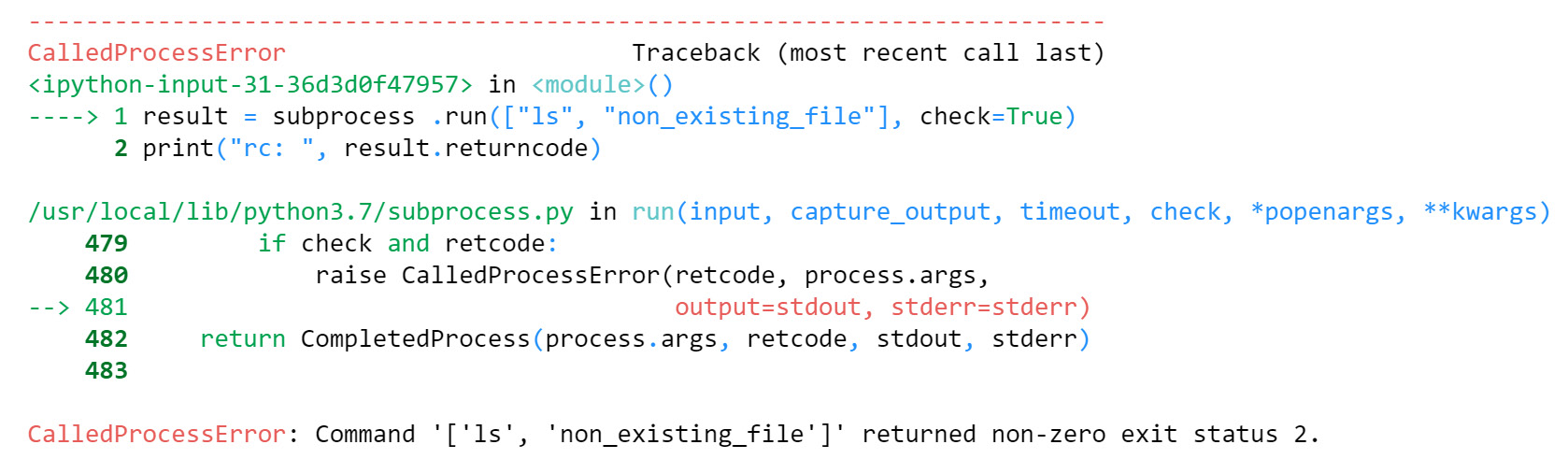
Figure 6.24: The result of running subprocess on a failed command

This is a great way to call other programs in which we just want them to be executed to have a look at the error, such as calling batch processing scripts or programs. The exceptions raised in those situations contain information such as the command that was run, the output if it was captured, and the return code.

The subprocess.run function also has some other interesting arguments that are helpful in some more special situations. As an example, if you are using subprocess.call with a program that expects any input through stdin, you can pass such input via the stdin argument. You can also pass a timeout for how many seconds you should wait for the program to finish. If the program does not return by that time, it will be terminated and, once finished, a timeout exception will be raised to inform us of the failure.

Processes created with the subprocess.run method will inherit the environment variables from the current process.

sys.executable is a string giving the absolute path of the executable binary for the Python interpreter on systems. If Python, is unable to retrieve the real path to its executable process, sys.executable will be an empty string or None.

Note

The -c option on the Python interpreter is for running code inline. You will be using this option in Activity 16: Testing Python Code.

You will see how you can customize child processes in the following exercise.

Exercise 92: Customizing Child Processes with env vars

As part of an auditing tool, you are asked to print our environment variables by using the subprocess module, without relying on the Python os.environ variable. However, you have to do so concealing our server name, as our manager does not want to show this information to our clients.

In this exercise, you will call other apps in the OS while changing the environment variables of the parent process. You will see how you can change environment variables when using subprocess:

1. Import subprocess.

   Bring the subprocess module into the current namespace:

   import subprocess

   You can also bring just the run command by running subprocess by importing run, but by importing this module itself, we can see the module name when we are calling run. Otherwise, you wouldn't know where the run was coming from. Additionally, subprocess defines some constants that are used for some arguments on the advanced use of Popen. By importing subprocess, you have all those available.

2. Run env to print the environment variables.

   You can run the env Unix command, which will list the process environment variables in stdout:

   result = subprocess.run(

       ["env"],

       capture_output=True,

       text=True

   )

   print(result.stdout)

   You pass capture_output and text to be able to read the stdout result in a Unicode string. You can confirm that the process indeed has a list of environment variables already set; those match the ones of the parent process:

   

   Figure 6.25: Output showing the environment variables using env

3. Use a different set of environment variables.

   If you wanted to customize the environment variables that our subprocess has, you could use the env keyword of the subprocess.run method:

   result = subprocess.run(

        ["env"],

       capture_output=True,

       text=True,

       env={"SERVER": "OTHER_SERVER"}

   )

   print(result.stdout)

   The output is as follows:

   

   Figure 6.26: Output showing a different set of environment variables

4. Now, modify the default set of variables.

   Most of the time, you just want to modify or add one variable, not just replace them all. Therefore what we did in the previous step is too radical, as tools might require environment variables that are always present in the OS.

   To do so, you will have to take the current process environment and modify it to match the expected result. We can access the current process environment variables via os.environ and copy it via the copy module. Though you can also use the dict expansion syntax with the keys that you want to change to modify it, as shown in the following example:

   import os

   result = subprocess.run(

       ["env"],

       capture_output=True,

       text=True,

       env={**os.environ, "SERVER": "OTHER_SERVER"}

   )

   print(result.stdout)

   The output is as follows:

Figure 6.27: Modifying the default set of environment variables

You can see that you now have the same environments in the process created with subprocess as those in the current process, but that you have modified SERVER.

You can use the subprocess module to create and interact with other programs installed on our OS. The subprocess.run function and its different arguments make it easy to interact with different kinds of programs, check their output, and validate their results. There are also more advanced APIs available through the subprocess.Popen call if they are needed.

Activity 16: Testing Python Code

A company that receives small Python code snippets from its clients with basic mathematical and string operations has realized that some of the operations crash their platform. There is some asked for code requested by clients that cause the Python interpreter to abort as it cannot compute it.

This is an example:

compile("1" + "+1" * 10 ** 6, "string", "exec")

You are therefore asked to create a small program that can run the requested code and check whether it will crash without breaking the current process. This can be done by running the same code with subprocess and the same interpreter version that is currently running the code.

To get this code, you need to:

1. Find out the executable of our interpreter by using the sys module.
2. Use subprocess to run the code with the interpreter that you used in the previous step.
3. Use the -c option of the interpreter to run code inline.
4. Check whether the result code is -11, which corresponds to an abort in the program.

   Note

   The solution for this activity is available on page 539.

In the following topic, you will be using logging, which plays a major part in the life of a developer.

Logging

Setting up an application or a library to log is not just good practice; it is a key task of a responsible developer. It is as important as writing documentation or tests. Many people consider logging the "runtime documentation"; the same way developers read the documentation when interacting with the DevOps source code, and other developers will use the log traces when the application is running.

Hardcore logging advocates state that debuggers are extremely overused, and people should rely more on logging, using both info and trace logs to troubleshoot their code in development.

The idea is that if you are not able to troubleshoot your code with the highest level of verbosity in development, then you may have issues in production that you won't be able to figure out the root issue of.

Using Logging

Logging is the best way to let the users of the running application know which state the process is in, and how it is processing its work. It can also be used for auditing or troubleshooting client issues. There is nothing more frustrating than trying to figure out how your application behaved last week and having no information at all about what happened when it faced an issue.

You should also be careful about what information we log. Many companies will require users to never log information such as credit cards or any sensitive user data. Whilst it is possible to conceal such data after it is logged, it is better to be mindful when we log it.

You might wonder what is wrong with just using print statements, but when you start to write large-scale applications or libraries, you realize that just using print does nothing to instrument an application. By using the logging module, you also get the following:

• Multithreading support: The logging module is designed to work in multithreaded environments. This is needed when using multiple threads as, otherwise, the data that you log will get interleaved, as can happen with print.
• Categorization through multiple levels of logging: When using print, there is no way to transmit the importance of the log trace being emitted. By using logging, we can choose the category that we want to log under to transmit the importance of it.
• Separation of concerns between instrumentation and configuration: There are two different users of the logging library — users who just emit and those who configure the logging stack. The logging library separates those nicely, allowing libraries and applications to just instrument their code with logs at different levels, and the final user to configure the logging stack at will.
• Flexibility and configurability: The logging stack is easily extensible and configurable. There are many types of handlers, and it is trivial to create new classes that extend its functionality. There is even a cookbook on how to extend the logging stack in the standard library documentation.

The main class you interact with when using the logging library is logger. can be used to emit logs in any category. You usually create loggers by getting them through the logging.getLogger(<logger name>) factory method.

Once you have a logger object, you can call the different logging methods that match the different default categories that you are able to log in:

• debug: Fine-grained messages that are helpful for debugging and troubleshooting applications, usually enabled in development. As an example, a web server will log the input payload when receiving a request at this level.
• info: Coarse-grained informational messages that highlight the progress of an application. As an example, a web server will emit the requests being handled at this level without details of the data being received.
• warning: Messages that inform the user of a potentially harmful situation in the application or library. In our example of a web server, this will happen if you fail to decode an input JSON payload because it is corrupted. Note that while it might feel like an error and it might be for the whole system, if you own the frontend as well, the issue is not in the application handling the request; it is in the process sending it. Therefore, a warning might help notify the user of such an issue, but it is not an error. The error should be reported to the client as an error response, and the client should handle it as appropriate.
• error: Used for situations where an error has taken place, but the application can continue to function properly. Logging an error usually means there is an action that needs to be carried out by a developer in the source code that logged it. Logging errors commonly happen when you capture an exception, and you have no way of handling it effectively. It is quite common to set up alerts in connection with errors to inform the DevOps or developer that an error situation took place. In our web server application, this might happen if you fail to encode a response or an exception is raised that was not expected when handling the request.
• fatal: Fatal logs indicate that there has been an error situation that compromises the current stability of the program, and, quite often, the process is restarted after a fatal message is logged. A fatal log means that the application needs an operator to take action urgently, compared to an error that a developer is expected to handle. A common situation is when the connection to a database is lost, or any other resource that is key for the application is no longer reachable.

Logger Object

Loggers have a hierarchy of names split by a dot. For example, if you ask for a logger named my.logger, you are creating a logger that is a child of my, which is a child of the root logger. All top-level loggers "inherit" from the root logger.

You can get the root logger by calling getLogger without arguments or by logging directly with the logging module. A common practice is to use __name__ as the logger module. This makes your logging hierarchy follow your source code hierarchy. Unless you have a strong reason not to do that, use __name__ when developing libraries and applications.

Exercise 93: Using a logger Object

The goal of this exercise is to create a logger object and use four different methods that allow us to log in the categories mentioned in the Logging section:

1. Import the logging module:

   import logging

2. Create a logger.

   We can now get a logger through the factory method getLogger:

   logger = logging.getLogger("logger_name")

   This logger object will be the same everywhere, and you call it with the same name.

3. Log with different categories:

   logger.debug("Logging at debug")

   logger.info("Logging at info")

   logger.warning("Logging at warning")

   logger.error("Logging at error")

   logger.fatal("Logging at fatal")

   The output is as follows:

   

   Figure 6.28: The output of running logging

   By default, the logging stack will be configured to log warnings and above, which explains why you only see those levels being printed to the console. You will see later how to configure the logging stack to include other levels, such as info. Use files or a different format to include further information.

4. Include information when logging:

   system = "moon"

   for number in range(3):

       logger.warning("%d errors reported in %s", number, system)

   Usually, when you log, you don't pass just a string, but also some variable or information that helps us with the current state of the application:

Figure 6.29: The output of running warning logs

Note

You use Python standard string interpolation, and you pass the remainder of the variables as attributes. %d is used to format numbers, while %s is used for strings. The string interpolation format also has syntax to customize the formatting of numbers or to use the repr of an object.

After this exercise, you now know how to use the different logger methods to log in different categories depending on the situation. This will allow you to properly group and handle your application messages.

Logging in warning, error, and fatal Categories

You should be mindful when you log in warning, error, and fatal. If there is something worse than an error, it is two errors. Logging an error is a way of informing the system of a situation that needs to be handled, and if you decide to log an error and raise an exception, you are basically duplicating the information. As a rule of thumb, following these two pieces of advice is key to an application or library that logs errors effectively:

• Never ignore an exception that transmits an error silently. If you handle an exception that notifies you of an error, log that error.
• Never raise and log an error. If you are raising an exception, the caller has the ability to decide whether it is truly an error situation, or whether they were expecting the issue to occur. They can then decide whether to log it following the previous rule, to handle it, or to re-raise it.

A good example of where the user might be tempted to log an error or warning is in the library of a database when a constraint is violated. From the library perspective, this might look like an error situation, but the user might be trying to insert it without checking whether the key was already in the table. The user can therefore just try to insert and ignore the exception, but if the library code logs a warning when such a situation happens, the warning or error will just spew the log files without a valid reason. Usually, a library will rarely log an error unless it has no way of transmitting the error through an exception.

When you are handling exceptions, it is quite common to log them and the information they come with. If you want to include the exception and trace back the full information, you can use the exc_info argument in any of the methods that we saw before:

try:

    int("nope")

except Exception:

    logging.error("Something bad happened", exc_info=True)

The output is as follows:

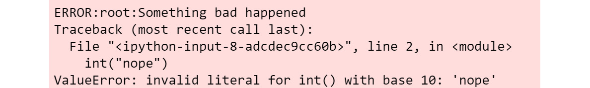
Figure 6.30: Example output when logging an exception with exc_info.

The error information now includes the message you passed in, but also the exception that was being handled with the traceback. This is so useful and common that there is a shortcut for it. You can call the exception method to achieve the same as using error with exc_info:

try:

    int("nope")

except Exception:

    logging.exception("Something bad happened")

The output is as follows:

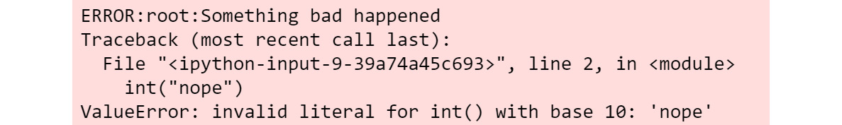
Figure 6.31: Example output when logging an exception with the exception method

Now, you will review two common bad practices with the logging module.

The first one is a greedy string formatting. You might see some linters complain about formatting a string by the user, rather than relying on the logging module's string interpolation. This means that logging.info("string template %s", variable) is preferred over logging.info("string template {}".format(variable)). This is the case since, if you perform the string interpolation with the format, you will be doing it no matter how we configure the logging stack. If the user who configures the application decides that they don't need to print out the logs in the information level, you will have to perform interpolation, when it wasn't necessary:

# prefer

logging.info("string template %s", variable)

# to

logging.info("string template {}".format(variable))

Note

Linters are programs that detect code style violations, errors, and suggestions for the user.

The other, more important, bad practice is capturing and formatting exceptions when it's not really needed. Often, you see developers capturing broad exceptions and formatting them manually as part of a log message. This is not only boilerplate but also less explicit. Compare the following two approaches:

d = dict()

# Prefer

try:

    d["missing_key"] += 1

except Exception:

    logging.error("Something bad happened", exc_info=True)

# to

try:

    d["missing_key"] += 1

except Exception as e:

    logging.error("Something bad happened: %s", e)

The output is as follows:

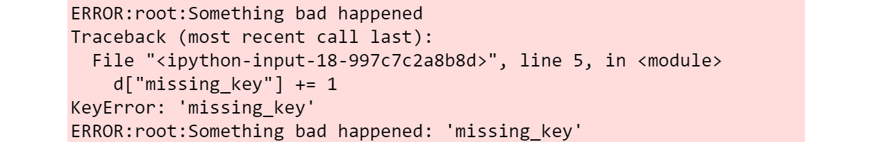
Figure 6.32: Example output difference of exc_info versus logging an exception string

The output in the second approach will only print the text of the exception, without further information. We don't know if it was a key error, nor where the issue appeared. If the exception was raised without a message, we would just get an empty message. Additionally, if logging an error, use an exception, and you won't need to pass exc_info.

Configuring the Logging Stack

Another part of the logging library is the functions to configure it, but before diving into how to configure the logging stack, you should understand its different parts and the role they play.

You've already seen logger objects, which are used to define the logging messages that need to be generated. There are also the following classes, which take care of the process of processing and emitting a log:

• Log Records: This is the object that is generated by the logger and contains all the information about the log, including the line where it was logged, the level, the template, and arguments, among others.
• Formatters: These take log records and transform them into strings that can be used by handlers that output to streams.
• Handlers: These are the ones that actually emit the records. They frequently use a formatter to transform records into strings. The standard library comes with multiple handlers to emit log records into stdout, stderr, files, sockets, and so on.
• Filters: Tools to fine-tune log record mechanisms. They can be added to both handlers and loggers.

If the functionality that is already provided by the standard library is not enough, you can always create our own kind of classes that customize how the logging process is performed.

Note

The logging library is truly flexible. If you are interested in doing so, read through the logging cookbook in the Python official documentation to see some examples at https://docs.python.org/3/howto/logging-cookbook.html.

Armed with this knowledge, there are multiple ways to configure all of the elements of the logging stack. You can do so by plugging together all the classes manually with code, passing a dict via logging.config.dictConfig, or through an ini file with logging.config.iniConfig.

Exercise 94: Configuring the Logging Stack

In this exercise, you will learn how to configure the logging stack through multiple methods to output log messages to stdout.

You want to configure the logging stack to output logs to the console, which should look like this:

Figure 6.33: Outputting logs to the console

Note

The background is white, which means the output went to stdout and not stderr, as in the previous examples. Make sure to restart the kernel or interpreter every time prior to configuring the logging stack.

You will see how you can configure it with code, with a dictionary, with basicConfig, and with a config file:

1. Open a new Jupyter notebook.
2. Start with configuring the code.

   The first way to configure the stack is by manually creating all the objects and plugging them together:

   import logging

   import sys

   root_logger = logging.getLogger()

   handler = logging.StreamHandler(sys.stdout)

   formatter = logging.Formatter("%(levelname)s: %(message)s")

   handler.setFormatter(formatter)

   root_logger.addHandler(handler)

   root_logger.setLevel("INFO")

   logging.info("Hello logging world")

   The output will be as follows:

   INFO: Hello logging world

   In this code, you get a handle of the root logger in the third line by calling getLogger without any arguments. You then create a stream handler, which will output to sys.stdout (the console) and a formatter to configure how we want the logs to look. Finally, you just need to bind them together by setting the formatter in the handler and the handler in the logger. You set the level in the logger, though you could also configure it in the handler.

3. Restart the kernel on Jupyter and now use dictConfig to achieve the same configuration:

   Exercise94.ipynb

   import logging

   from logging.config import dictConfig

   dictConfig({

       "version": 1,

       "formatters": {

           "short":{

               "format": "%(levelname)s: %(message)s",

           }

       },

       "handlers": {

          "console": {

               "class": "logging.StreamHandler",

               "formatter": "short",

               "stream": "ext://sys.stdout",

   https://packt.live/33U0z3D

   Note

   If the above link does not render, use https://nbviewer.jupyter.org/

   The output will be as follows:

   INFO: Hello logging world

   The dictionary configuring the logging stack is identical to the code in step 1. Many of the configuration parameters that are passed in as strings can also be passed as Python objects. For example, you can use sys.stdout instead of the string passed to the stream option or logging.INFO rather than INFO.

   Note

   The code in Step 3 is identical to the code in Step 2; it just configures it in a declarative way through a dictionary.

4. Now, again, restart the kernel on Jupyter and use basicConfig as mentioned in the following code snippet:

   import sys

   import logging

   logging.basicConfig(

       level="INFO",

       format="%(levelname)s: %(message)s",

       stream=sys.stdout

   )

   logging.info("Hello there!")

   The output will be as follows:

   INFO: Hello there!

   The logging stack comes with a utility function, basicConfig, which can be used to perform some basic configurations, such as the one we're performing here, as mentioned in the code snippet that follows.

5. Using an ini file.

   Another way to configure the logging stack is by using an ini file. We require an ini file, as follows:

logging-config.ini

[loggers]

keys=root

[handlers]

keys=console_handler

[formatters]

keys=short

[logger_root]

level=INFO

handlers=console_handler

[handler_console_handler]

class=StreamHandler

https://packt.live/32727X3

Note

If the above link does not render, use https://nbviewer.jupyter.org/

You can then load it with the following code:

import logging

from logging.config import fileConfig

fileConfig("logging-config.ini")

logging.info("Hello there!")

The output will be as follows:

INFO: Hello there!

All applications should configure the logging stack only once, ideally at startup. Some functions, such as basicConfig, will not run if the logging stack has already been configured.

You now know all of the different ways to configure an application's logging stack. This is one of the key parts of creating an application.

In the next topic, you will learn about collections.

Collections

You read about built-in collections in Chapter 2, Python Structures. You saw list, dict, tuple, and set, but sometimes, those collections are not enough. The Python standard library comes with modules and collections that provide a number of advanced structures that can greatly simplify our code in common situations. Now, you will explore how you can use counters, defauldict, and chainmap.

Counters

A counter is a class that allows us to count hashable objects. It has keys and values as a dictionary (it actually inherits from dict) to store objects as keys and the number of occurrences in values. A counter object can be created either with the list of objects that you want to count or with a dictionary that already contains the mapping of objects to their count. Once you have a counter instance created, you can get information about the count of objects, such as getting the most common ones or the count of a specific object.

Exercise 95: Counting Words in a Text Document

In this exercise, you will use a counter to count the occurrences of words in the text document https://packt.live/2OOaXWs:

1. Get the list of words from https://packt.live/2OOaXWs, which is our source data:

   import urllib.request

   url = 'https://www.w3.org/TR/PNG/iso_8859-1.txt'

   response = urllib.request.urlopen(url)

   words = response.read().decode().split()

   len(words)  # 858

   Here, you are using urllib, another module within the standard library, to get the contents of the URL of https://packt.live/2OOaXWs. You can then read the content and split it based on spaces and break lines. You will be using words to play with the counter.

2. Now, create a counter:

   import collections

   word_counter = collections.Counter(words)

   This creates a counter with the list of words passed in through the words list. You can now perform the operations you want on the counter.

   Note

   As this is a subclass of the dictionary, you can perform all the operations that you can also perform on the dictionary.

3. Get the five most common words:

   for word, count in word_counter.most_common(5):

       print(word, "-", count)

   You can use the most_common method on the counter to get a list of tuples with all the words and the number of occurrences. You can also pass a limit as an argument that limits the number of results:

   

   Figure 6.34: Getting the five common words as output

4. Now, explore occurrences of some words, as shown in the following code snippet:

   print("QUESTION", "-", word_counter["QUESTION"])

   print("CIRCUMFLEX", "-", word_counter["CIRCUMFLEX"])

   print("DIGIT", "-", word_counter["DIGIT"])

   print("PYTHON", "-", word_counter["PYTHON"])

   You can use the counter to explore the occurrences of specific words by just checking them with a key. Now check for QUESTION, CIRCUMFLEX, DIGIT, and PYTHON:

   

Figure 6.35: Output exploring the occurrences of some words

Note how you can just query the counter with a key to get the number of occurrences. Something else interesting to note is that when you query for a word that does not exist, you get 0. Some users might have expected a KeyError.

In this exercise, you just learned how to get a text file from the internet and perform some basic processing operations, such as counting the number of words.

defaultdict

Another class that is considered to create simpler-to-read code is the defaultdict class. This class behaves like a dict but allows you to provide a factory method to be used when a key is missing. This is extremely useful in multiple scenarios where you edit values, and especially if you know how to generate the first value, such as when you are building a cache or counting objects.

In Python, whenever you see code like the following code snippet, you can use defaultdict to improve the code quality:

d = {}

def function(x):

    if x not in d:

        d[x] = 0 # or any other initialization

    else:

        d[x] += 1 # or any other manipulation

Some people will try to make this more Pythonic by using EAFP over LBYL, which handles the failure rather than checking whether it will succeed:

d = {}

def function(x):

    try:

        d[x] += 1

    except KeyError:

        d[x] = 1

While this is indeed the preferred way to handle this code according to Python developers as it better conveys the information that the main part of the logic is the successful case, the correct solution for this kind of code is defaultdict. Intermediate to advanced Python developers will immediately think of transforming that code into a default dict and then comparing how it looks:

import collections

d = collections.defaultdict(int)

def function(x):

    d[x] += 1

The code becomes trivial, and it is identical to what you saw in the two previous examples. defaultdict is created with a factory method that will just call int() if the key is missing, which returns 0 and is incremented by one. It is a simply beautiful piece of code. But note that defaultdict can be used in other ways; the function passed to its constructor is a callable factory method. You use int not as a type, but as a function that is called. In the same way, you could pass list, set, or any callable you want to create.

Exercise 96: Refactoring Code with defaultdict

In this exercise, you will learn how to refactor code and simplify it by using defaultdict:

_audit = {}

def add_audit(area, action):

    if area in _audit:

        _audit[area].append(action)

    else:

        _audit[area] = [action]

        

def report_audit():

    for area, actions in _audit.items():

        print(f"{area} audit:")

        for action in actions:

            print(f"- {action}")

        print()

Note

The aforementioned code can be found on GitHub: https://packt.live/31ccJ6k.

The code template mentioned earlier in this exercise keeps an audit of all the actions that are performed in a company. They are split by area and the dictionary that was used. You can clearly see in the add_audit function the pattern we spoke about before. You will see how you can transform that into simpler code by using defaultdict and how it could be later extended in a simpler way:

1. Run the code that keeps an audit of all the actions, as mentioned previously.

   First, run the code to see how it behaves. Before doing any refactoring, you should understand what you are trying to change, and ideally, have tests for it

   add_audit("HR", "Hired Sam")

   add_audit("Finance", "Used 1000£")

   add_audit("HR", "Hired Tom")

   report_audit()

   You should get the following output:

   

   Figure 6.36: Output showing the code keeping an audit of the changes

   You can see that this works as expected, and you can add items to the audit and report them.

2. Introduce a default dict.

   You can change dict for defaultdict and just create a list whenever you try to access a key that does not exist. This will need to be done only in the add_audit function. As report_audit uses the object as a dictionary and defaultdict is a dictionary, you don't need to change anything in that function. You will see how it will look in the following code snippet:

   import collections

   _audit = collections.defaultdict(list)

   def add_audit(area, action):

       _audit[area].append(action)

           

   def report_audit():

       for area, actions in _audit.items():

           print(f"{area} audit:")

           for action in actions:

               print(f"- {action}")

           print()

   Note

   The add_audit function has become a single line. It just appends an action to an area.

   When a key is not found in the _audit object, our defaultdict just calls the list method, which returns an empty list. The code could not be any simpler.

   What about if you are asked to log the creation of an area in the audit? Basically, whenever a new area is created in our audit object, to have an element present. The developer that initially wrote the code claims that it was easier to change with the old layout, without using defaultdict.

3. Use the add_audit function to create the first element.

   The code without defaultdict for add_audit will be as follows:

   def add_audit(area, action):

       if area not in _audit:

           _audit[area] = ["Area created"]

       _audit[area].append(action)

   The code change performed in add_audit is much more complex than the one you will have to perform in your function with defaultdict.

   With defaultdict, you just need to change the factory method from being a list to being a list with the initial string:

   import collections

   _audit = collections.defaultdict(lambda: ["Area created"])

   def add_audit(area, action):

       _audit[area].append(action)

           

   def report_audit():

       for area, actions in _audit.items():

           print(f"{area} audit:")

           for action in actions:

               print(f"- {action}")

           print()

   And it is still simpler than without defaultdict:

   add_audit("HR", "Hired Sam")

   add_audit("Finance", "Used 1000£")

   add_audit("HR", "Hired Tom")

   report_audit()

   You should get the following output:

Figure 6.37: Output with a function to create the first element

At the end of this exercise, you now know how to use defaultdict with multiple different factory methods. This is useful when writing Pythonic code and simplifying existing code bases.

ChainMap

Another interesting class in the collection's module is ChainMap. ChainMap is a structure that allows you to combine lookups for multiple mapping objects, usually dictionaries. It can be seen as a multi-level object; the user can see the front of it with all the keys and all the mappings, but the keys that map on the frontend hide the mappings on the backend.

Say you want to create a function that returns the menu our users will have at a restaurant; the function just returns a dictionary with the different types of elements of the lunch and the value of them. You want to allow our users to customize any part of the lunch, but you also want to provide some defaults. This can easily be done with ChainMap:

import collections

_defaults = {

    "apetisers": "Hummus",

    "main": "Pizza",

    "desert": "Chocolate cake",

    "drink": "Water",

}

def prepare_menu(customizations):

    return collections.ChainMap(customizations, _defaults)

def print_menu(menu):

    for key, value in menu.items():

        print(f"As {key}: {value}.")

Note

You have a dictionary that provides you with the defaults, and you are combining it with the user's customizations by using ChainMap. The order is important, as it makes the user's dictionary values appear before the defaults and, if desired, you can also have more than two dictionaries, which might be useful for other use cases.

You will now see how chainmap behaves when you pass in different values:

menu1 = prepare_menu({})

print_menu(menu1)

The output is as follows:

Figure 6.38: Chainmap outputting different values

If the user passes in no customization, you get the default menu. All keys and values are taken from the _default dictionary that we provided:

menu3 = prepare_menu({"side": "French fries"})

print_menu(menu3)

The output is as follows:

Figure 6.39: Output with no customization; that is, the default menu

When a user passes a dictionary that changes one of the keys that is present in the _default dictionary, the value of the second dictionary is shadowed by the first one. You can see how the drink is now Red Wine rather than Water:

menu2 = prepare_menu({"drink": "Red Wine"})

print_menu(menu2)

The output is as follows:

Figure 6.40: Value of the dictionary changed, changing the drink to red wine

Users can also pass in new keys, which will be reflected in ChainMap.

You might be tempted to think that this is just an over-complication of using the dictionary constructor and that the same could be achieved with an implementation like the following one:

def prepare_menu(customizations):

    return {**customizations, **_defaults}

But the semantics are different. That implementation would create a new dictionary, which would not allow changes to the user's customizations or the defaults. Say you wanted to change the defaults after you have created some menus, we can do this with the ChainMap implementation since the returned object is just a view of multiple dictionaries:

_defaults["main"] = "Pasta"

print_menu(menu3)

The output is as follows:

Figure 6.41: Output with changed default values

Note

You were able to change the main dish. Changes in any of the dict that is part of chainmap are visible when interacting with it.

The different classes in the collection modules allow the developer to write better code by using more appropriate structures. With the knowledge you have gained in this topic, try to explore others, such as deque or basic skeletons, to build your own containers. Using these classes effectively in many situations is what differentiates an experienced Python programmer from a beginner.

Functools

The final module of the standard library you are going to look at allows constructs with a minimal amount of code. In this topic, you are going to see how to use lru_cache and partial.

Caching with functools.lru_cache

Often, you have a function that is heavy to compute, in which you just want to cache results. Many developers will create their own caching implementation by using a dictionary, but that is error-prone and adds unnecessary code to our project. The functools module comes with a decorator — that is, functools.lru_cache, which is provided exactly for these situations. It is a recently used cache, with a max_size that is provided when the code is constructed. This means that you can specify a number of input values that you want to cache as a maximum, to limit the memory this function can take, or it can grow indefinitely. Once you reach the maximum number of different inputs that we want to cache, the input that was the least recently used will be thrown away in favor of a new call.

Additionally, the decorator provides some new methods in the function that can be used to interact with the cache. We can use cache_clear to remove all of the previous hits saved in cache or cache_info to get information about the hits and misses, so as to allow us to tune it if needed. The original function information is also offered for inspection, as with any properly decorated function, through the __wrapped__ decorator.

It is important to keep in mind that the LRU cache should be used only in functions. This is useful if we just want to reuse existing values or the side effect will not happen. As an example, we should not use the cache on a function that writes something into a file or sends a package to an endpoint, as those actions will not be performed once the function is called again with the same input, which is the main purpose of the cache.

Lastly, for the cache to be usable in a function, all objects being passed need to be hashable. This means that integers, frozensets, tuples, and so on are allowed, but not modifiable objects, such as dicts, sets, or lists.

Exercise 97: Using lru_cache to Speed Up Our Code

In this exercise, you will see how to configure a function to use cache with functools and to reuse the results from previous calls to speed up the overall process.

You use the lru cache function of the functools module to reuse values that a function has already returned without having to execute them again.

We will start with a function that is mentioned in the following code snippet, which simulates taking a long time to compute, and we will see how we can improve this:

import time

def func(x):

    time.sleep(1)

    print(f"Heavy operation for {x}")

    return x * 10

If we call this function twice with the same arguments, we will be executing the code twice to get the same result:

print("Func returned:", func(1))

print("Func returned:", func(1))

The output is as follows:

Figure 6.42: Output showing the same arguments by calling the function twice

We can see this in the output and the print within the function, which happens twice. This is a clear improvement in performance as, once the function is executed, future executions are practically free. Now, we will improve the performance in the steps that follow:

1. Add the lru cache decorator to the func function:

   The first step is to use the decorator on our function:

   import functools

   import time

   @functools.lru_cache()

   def func(x):

       time.sleep(1)

       print(f"Heavy operation for {x}")

       return x * 10

   When we execute the function for the same input, we now see that the code is executed only once, but we still get the same output from the function:

   print("Func returned:", func(1))

   print("Func returned:", func(1))

   print("Func returned:", func(2))

   The output is as follows:

   

   Figure 6.43: Output showing the code being executed once but with the same output

   Note

   The Heavy operation only happens once for 1. We are also calling 2 here to show that the value is different based on its input, and, since 2 was not cached before, it has to execute the code for it.

   This is extremely useful; with just one line of code, we have at hand a fully working implementation of an LRU cache.

2. Change the cache size using the maxsize argument.

   The cache comes with a default size of 128 elements, but this can be changed if needed, through the maxsize argument:

   import functools

   import time

   @functools.lru_cache(maxsize=2)

   def func(x):

       time.sleep(1)

       print(f"Heavy operation for {x}")

       return x * 10

   By setting it to 2, we are sure that only two different inputs will be saved. We can see this by using three different inputs and calling them in reverse order later:

   print("Func returned:", func(1))

   print("Func returned:", func(2))

   print("Func returned:", func(3))

   print("Func returned:", func(3))

   print("Func returned:", func(2))

   print("Func returned:", func(1))

   The output is as follows:

   

   Figure 6.44: Output with a changed cache size

   The cache successfully returned the previous values for the second call of 2 and 3, but the result for 1 was destroyed once 3 arrived, since we limited the size to two elements only.

3. Now, use it in other functions, such as lru_cache.

   Sometimes, the functions you want to cache are not in our control to change. If you want to keep both versions, that is, a cached and an uncached one, we can achieve this by using the lru_cache function just as a function and not as a decorator, as decorators are just functions that take another function as an argument:

   import functools

   import time

   def func(x):

       time.sleep(1)

       print(f"Heavy operation for {x}")

       return x * 10

   cached_func = functools.lru_cache()(func)

   Now, we can use either func or its cached version, cached_func:

   print("Cached func returned:", cached_func(1))

   print("Cached func returned:", cached_func(1))

   print("Func returned:", func(1))

   print("Func returned:", func(1))

   The output is as follows:

Figure 6.45: Output with the lru_cache function

We can see how the cached version of the function did not execute the code in the second call, but the uncached version did.

You just learned how to use functools to cache the values of a function. This is a really quick way to improve the performance of your application when applicable.

Partial

Another often used function in functools is partial. partial allows us to adapt existing functions by providing values for some of their arguments. It is like binding arguments in other languages, such as C++ or JavaScript, but this is what you would expect from a Python function. partial can be used to remove the need for specifying positional or keyword arguments, which makes it useful when we need to pass a function that takes arguments as a function that does not take them. Have look at some examples:

You will use a function that just takes three arguments and prints them:

def func(x, y, z):

    print("x:", x)

    print("y:", y)

    print("z:", z)

func(1, 2, 3)

The output is as follows:

Figure 6.46: The output, which simply prints the arguments

You can use partial to transform this function to take fewer arguments. This can be done in two ways, mainly, bypassing the arguments as a keyword, which is more expressive; or through positional arguments:

import functools

new_func = functools.partial(func, z='Wops')

new_func(1, 2)

The output is as follows:

Figure 6.47: Using partial to transform the output

You can call new_func without passing the z argument, as you have provided a value through the partial function. The z argument will always be set to the value provided when the function was created through the partial call.

If you decide to use positional only, the number of arguments you pass will bind from left to right, which means that if you only pass one argument, the x argument should no longer be provided:

import functools

new_func = functools.partial(func, 'Wops')

new_func(1, 2)

The output is as follows:

Figure 6.48: Output with positional arguments

Exercise 98: Creating a print Function That Writes to stderr

By using partial, you can also rebind the optional arguments to a different default, allowing us to change the default value that the function has. You will see how you can repurpose the print function to create a print_stderr function that just writes to stderr.

In this exercise, you will create a function that acts like print, but the output is stderr rather than stdout:

1. Explore the print argument.

   To start, you need to explore the arguments that print takes are. You will call help on print to see what the documentation offers:

   help(print)

   The output is as follows:

   

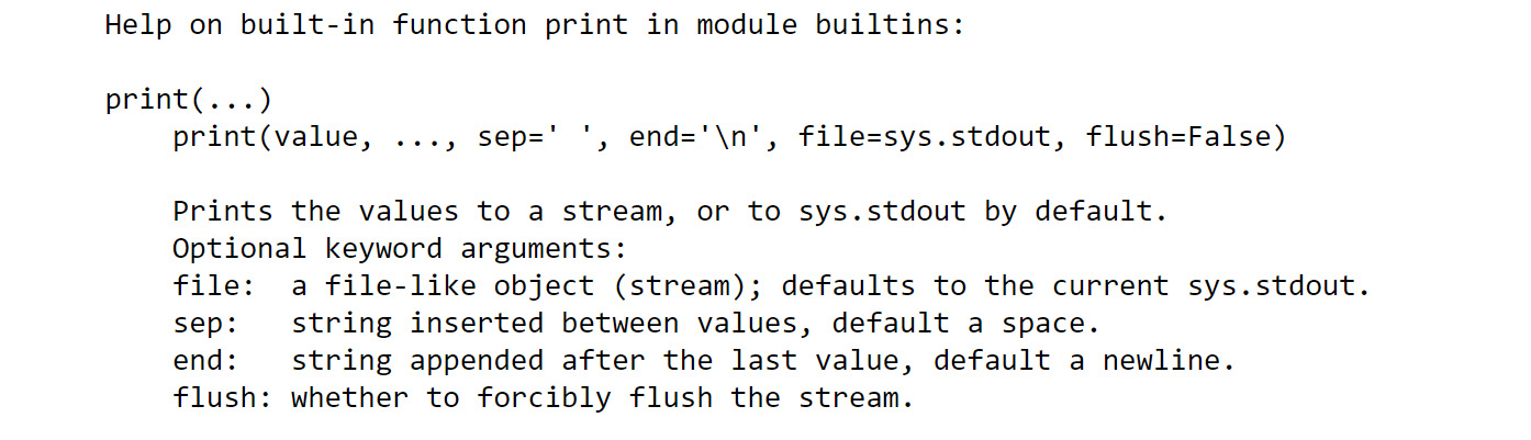
   Figure 6.49: Output with print arguments

   The argument that you are interested in is the file, which allows us to specify the stream you want to write to.

2. Print to stderr.

   Now, print the default value for the optional argument file, which is sysstdout, but you can pass sys.stderr to get the behavior you are looking for:

   import sys

   print("Hello stderr", file=sys.stderr)

   The output is as follows:

   

   Figure 6.50: Print to stderr output

   As you are printing to stderr, the output appears in red as expected.

3. Use partial to change the default.

   You can use partial to specify arguments to be passed and create a new function. You will bind file to stderr and see the output:

   import functools

   print_stderr = functools.partial(print, file=sys.stderr)

   print_stderr("Hello stderr")

   The output is as follows:

Figure 6.51: Print to stderr output through partial

Great – this works as expected; we now have a function that has changed the default value for the optional file argument.

Activity 17: Using partial on class Methods

Even though partial is an extremely useful and versatile function of the functools module, it seems to fail when we try to apply it to a class method.

To begin with, you are working in a company that models superheroes. You are asked to fix the following code snippet, as the previous developer attempted to use functools.partial to create the reset_name function but it does not seem to work well. Explore functools to make the following code snippet work without errors by creating partial on a class method.

In this activity, you will explore the partial module to see how partial can be used in more advanced use cases. This activity can be performed on the Jupyter notebook:

import functools

if __name__ == "__main__":

    class Hero:

        DEFAULT_NAME = "Superman"

        def __init__(self):

            self.name = Hero.DEFAULT_NAME

   

        def rename(self, new_name):

            self.name = new_name

   

        reset_name = functools.partial(rename, DEFAULT_NAME)

   

        def __repr__(self):

            return f"Hero({self.name!r})"

When we try to use partial in this class, to create the reset_name method, something seems to not work. Make the following succeed by modifying the way we used partial previously:

if __name__ == "__main__":

    hero = Hero()

    assert hero.name == "Superman"

    hero.rename("Batman")

    assert hero.name == "Batman"

    hero.reset_name()

    assert hero.name == "Superman"

Note

The aforementioned code can be found on GitHub: https://packt.live/33AxfPs

Steps:

1. Run the code and see what error it outputs.
2. Check for alternatives for functools.partial by running help (functools).
3. Use functools.partialmethod to implement the new class.

   Note

   The solution for this activity is available on page 540.

Summary

You have looked at multiple modules in the standard library and how they help you write well-tested and easier-to-read code. However, there are still many more modules to explore and understand in order to use them effectively, though. We have learned that Python comes with batteries included, through its vast standard library, and that, in many situations, the utilities it provides are extended through an advanced API. By having the mindset of checking how things can be solved with the standard library before trying to write our own code, you can become better Python programmers.

Now that you have some knowledge of the standard library, you will start to look more deeply into how to make our code easier to read for Python programmers, usually known as Pythonic code. While using the standard library as much as possible is a good start, there are some other tips and tricks that we will look at in Chapter 7, Becoming Pythonic.