
Overview
In this chapter, we will introduce the popular Multi-Armed Bandit problem and some common algorithms used to solve it. We will learn how to implement some of these algorithms, such as Epsilon Greedy, Upper Confidence Bound, and Thompson Sampling, in Python via an interactive example. We will also learn about contextual bandits as an extension of the general Multi-Armed Bandit problem. By the end of this chapter, you will have a deep understanding of the general Multi-Armed Bandit problem and the skill to apply some common ways to solve it.
Introduction
In the previous chapter, we discussed the technique of temporal difference learning, a popular model-free reinforcement learning algorithm that predicts a quantity via the future values of a signal. In this chapter, we will focus on another common topic, not only in reinforcement learning but also in artificial intelligence and probability theory – the Multi-Armed Bandit (MAB) problem.
Framed as a sequential decision-making problem to maximize the reward while playing at the slot machines in a casino, the MAB problem is highly applicable for any situation where sequential learning under uncertainty is needed, such as A/B testing or designing recommender systems. In this chapter, we will be introduced to the formalization of the problem, learn about the different common algorithms as solutions to the problem (namely Epsilon Greedy, Upper Confidence Bound, and Thompson Sampling), and finally implement them in Python.
Overall, this chapter will offer you a deep understanding of the MAB problem in different contexts of sequential decision-making and offer you the opportunity to apply that knowledge to solve a variation of the problem called the queueing bandit.
First, let's begin by discussing the background and the theoretical formulation of the problem.
Formulation of the MAB Problem
In its most simple form, the MAB problem consists of multiple slot machines (casino gambling machines), each of which can return a stochastic reward to the player each time it is played (specifically, when its arm is pulled). The player, who would like to maximize their total reward at the end of a fixed number of rounds, does not know the probability distribution or the average reward that they will obtain from each slot machine. The problem, therefore, boils down to the design of a learning strategy where the player needs to explore what possible reward values each slot machine can return and from there, quickly identify the one that is most likely to return the greatest expected reward.
In this section, we will briefly explore the background of the problem and establish the notation and terminology that we will be using throughout this chapter.
Applications of the MAB Problem
The slot machines we mentioned earlier are just a simplification of our settings. In the general case of a MAB problem, we are faced with a set of multiple decisions that we can choose from at each step, and we need to sufficiently explore each of the decisions so that we become more informed about the environment we are in, all while making sure we converge on the optimal decision soon so that our total reward is maximized at the end of the process. This is the classic trade-off between exploration and exploitation we are faced with in common reinforcement learning problems.
Popular applications of the MAB problem include recommender systems, clinical trials, network routing, and as we will see at the end of this chapter, queueing theory. Each of these applications contains the quintessential characteristics that define the MAB problem: at each step of a sequential process, a decision-maker needs to select from a predetermined set of possible choices and, depending on the past observations, the decision-maker needs to find a balance between exploring different choices and exploiting the one that they believe is the most beneficial.
As an example, one of the goals of recommender systems is to display the products that their customers are most likely to consider/buy. When a new customer logs into a system such as a shopping website or an online streaming service, the recommender system can observe the customer's past behaviors and choices and make a decision regarding what kind of product advertisement should be shown to the customer. It does this so that the probability that they click on the advertisement is maximized.
As another example, which we will see in more detail later on, in a queueing system consisting of multiple customer classes, each is characterized by an unknown service rate. The queue coordinator needs to figure out how to best order these customers so that a given objective, such as the cumulative waiting time of the whole queue, is optimized.
Overall, MAB is an increasingly ubiquitous problem in artificial intelligence and, specifically, reinforcement learning that has many interesting applications. In the next section, we will officially formalize the problem and the terminologies that we will be using throughout this chapter.
Background and Terminology
A MAB problem is characterized by the following elements:
- A set of "K" actions to choose from. Each of these actions is called an arm, following the colloquial terminology with respect to slot machines.
- A central decision-maker who needs to choose between this set of actions at each step of the process. We call the act of choosing an action pulling an arm, and the decision-maker the player.
- When one of the "K" available arms is pulled, the player receives a stochastic, or random, reward drawn from a probability distribution that is specific to that arm. It is important that the rewards are randomly chosen from their respective distributions; if they were otherwise fixed, the player could identify the arm that will return the highest reward quickly and the problem would become less interesting.
- The goal of the player is, again, to choose one of the "K" arms during each step of a running process so that their reward is maximized at the end. The number of steps in the process is called the horizon, which may or may not be known by the player beforehand.
- In most cases, each arm can be pulled infinitely. When the player is certain that a specific arm is the optimal one, they can keep choosing that arm for the rest of the process without deviating. However, in various settings, the number of times an arm can be pulled is finite, thus increasing the complexity of the problem.
The following diagram visualizes an iterative step in the environment that we are working with, where we have four arms whose success rates are estimated as 70%, 30%, 55%, and 40%.
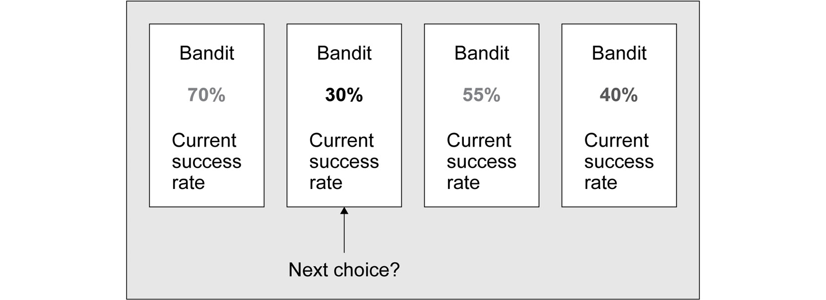
Figure 8.1: A typical MAB iteration
At each step, we need to make a decision about which arm we should choose to pull next:
- Opposite to the language of reward and the corresponding maximization objective, a MAB problem can also be framed in the context of a cost minimization objective. The queueing example can, once again, be used: the cumulative waiting time of the whole queue is a negative quantity, or in other words, the cost that needs to be minimized.
- It is common to compare the performance of a strategy to the optimal strategy or the genie strategy, which knows ahead of time what the optimal arm to pull is and always pulls that arm at every step of the process. Of course, it is highly improbable that any real learning strategy can simulate the performance of the genie strategy, but it does provide us with a fixed metric to compare our approaches against. The difference in performance of a given strategy and the genie strategy is known as the regret, which is to be minimized.
The central question of a MAB problem is how to identify the arm with the greatest expected reward (or lowest expected cost) with minimal exploration (pulling the suboptimal arms). This is because the more the player explores, the less frequent their choice of the optimal arm becomes, and the more their final reward decreases. However, if the player does not sufficiently explore all the arms, chances are they will misidentify the optimal arm and their total reward will be negatively affected in the end.
These situations arise when the stochastic rewards of the true optimal arm appear to be lower than those from other arms in the first few examples (due to randomness), causing the player to misidentify the optimal arm. Depending on the actual reward distribution that each arm has, this event can be quite likely to happen.
So, that is the general problem we set out to solve in this chapter. We now need to briefly consider the concept of probability distributions of reward in the context of MAB in order to fully understand the problem we are trying to solve.
MAB Reward Distributions
In the traditional MAB problem, the reward from each arm of the bandit is associated with a Bernoulli distribution. Each Bernoulli distribution is, in turn, parameterized by a non-negative number, p, that is, at most, 1. When a number is drawn from a Bernoulli distribution, it can take on two possible values: 1, which has a probability of p, and 0, which consequently has a probability of 1 - p. A high value of p therefore corresponds to a good arm for the player to pull. This is because the player is more likely to receive 1 as their reward. Of course, a high value of p does not guarantee that the reward obtained from a specific arm is always 1, and chances are, out of many pulls from even the arm with the highest value of p (in other words, the optimal arm), some of the rewards will be 0.
The following diagram is an example of a Bernoulli bandit setting:
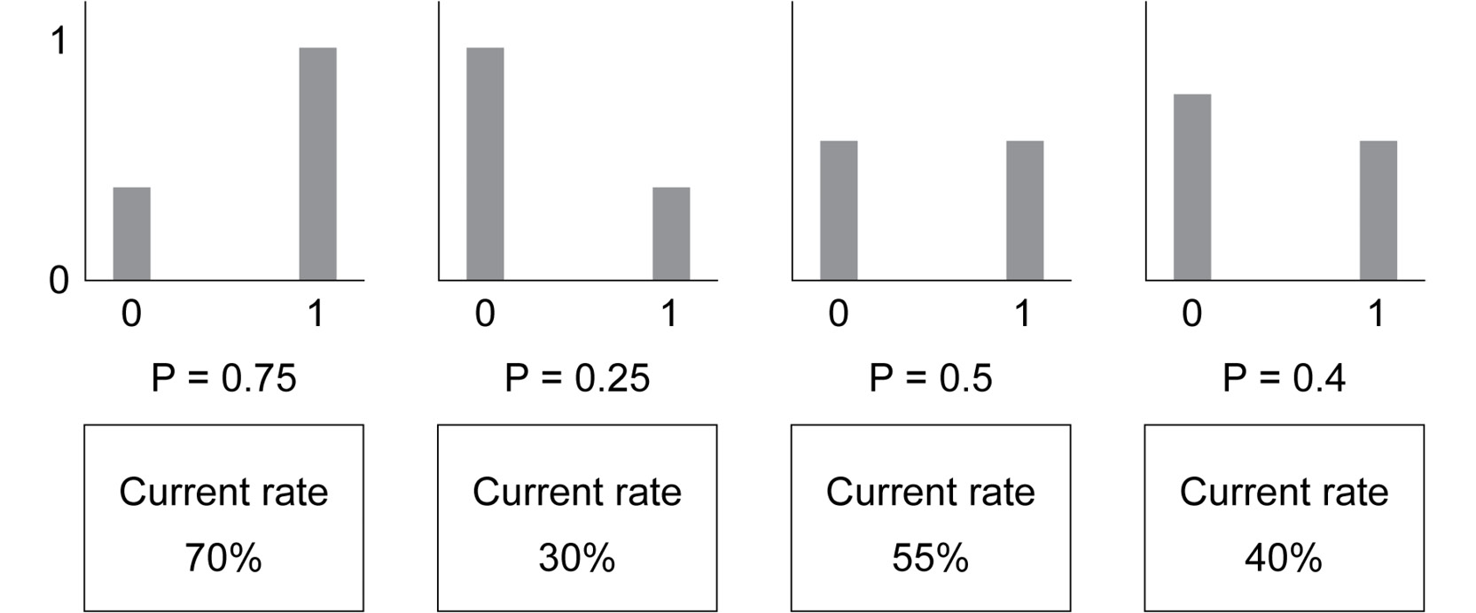
Figure 8.2: Sample Bernoulli MAB problem
Each arm has its own reward distribution: the first has a true probability of 75% of returning 1 and 25% of returning 0, the second has 25% for 1 and 75% for 0, and so on. Note that the rates that we empirically observe do not always match the true rates.
From here, we can generalize a MAB problem where the reward of an arm follows any probability distribution. While the inner workings of these distributions are different, the goal of a MAB algorithm remains constant: identifying the arm associated with the distribution with the highest expectation in order to maximize the final cumulative reward.
Throughout this chapter, we will be working with Bernoulli-distributed rewards, as they are among the most natural and intuitive reward distributions and will provide us with the context in which we can study various MAB algorithms. Finally, before we consider the different algorithms that will be covered in this chapter, let's take a moment to familiarize ourselves with the programming interface that we will be working with.
The Python Interface
The Python environment that will help facilitate our discussions of MAB algorithms is included in the utils.py file of this chapter's code repository on GitHub: https://packt.live/3cWiZ8j.
From this file, we can import the Bandit class into a separate script or a Jupyter script. This class is the interface we will use to create, interact, and solve various MAB problems. If the code we are working with is in the same directory as this file, we can import the Bandit class by simply using the following code:
from utils import Bandit
Then, we can declare an MAB problem as an instance of a Bandit object:
my_bandit = Bandit()
Since we are not passing any arguments to this declaration, this Bandit instance takes on its default value: an MAB problem with two Bernoulli arms with probabilities of 0.7 and 0.3 (although our algorithms technically cannot know this).
The most integral method of the Bandit class that we need to be aware of is pull(). This method takes in an integer as an argument, denoting the index of the arm we would like to pull at a given step, and returns a number representing the stochastic reward drawn from the distribution associated with that same arm.
For example, in the following code snippet, we call this pull() method with the 0 parameter to pull the first arm and record the returned reward, like so:
reward = my_bandit.pull(0)
reward
Here, you might see the number 0 or the number 1 printed out, which denotes the reward that you receive by pulling arm 0. Say we'd like to pull arm 1 once; the same API can be used:
reward = my_bandit.pull(1)
reward
Again, the output might be 0 or 1 since we are drawing from a Bernoulli distribution.
Say we'd like to inspect what the reward distribution of each arm might look like, or more specifically, which out of the two arms is the one more likely to return more reward. To do this, we pull from each arm 10 times and record the returned reward at each step:
running_rewards = [[], []]
for _ in range(10):
running_rewards[0].append(my_bandit.pull(0))
running_rewards[1].append(my_bandit.pull(1))
running_rewards
This code produces the following output:
[[1, 1, 1, 0, 0, 1, 1, 1, 0, 0], [0, 0, 1, 0, 0, 1, 0, 1, 1, 1]]
Again, due to randomness, you might get a different output. Considering the preceding output, we can see that arm 0 returned a positive reward 6 out of 10 pulls, while arm 1 returned a positive reward 5 times.
We'd also like to plot the cumulative reward throughout the process of 20 steps from each arm. Here, we can use the np.cumsum() function from the NumPy library to compute that quantity and plot it using the Matplotlib library, like so:
rounds = [i for i in range(1, 11)]
plt.plot(rounds, np.cumsum(running_rewards[0]),
label='Cumulative reward from arm 0')
plt.plot(rounds, np.cumsum(running_rewards[1]),
label='Cumulative reward from arm 1')
plt.legend()
plt.show()
The following graph will then be produced:

Figure 8.3: Sample graph of cumulative reward
This graph allows us to visually inspect how fast the cumulative reward we receive from each arm grew throughout the process of 10 pulls. We can also see that the cumulative reward from arm 0 is always greater than that from arm 1, indicating that out of the two arms, arm 0 is the optimal one. This is consistent with the fact that arm 0 was initialized with a Bernoulli reward distribution where p = 0.7, and arm 1 has one where p = 0.3.
The pull() method is the lower-level API that facilitates processing at each step. However, when we design various MAB algorithms, we will be allowing the algorithms to interact with the bandit problem automatically, on their own, without any human interference. This leads us to the second method from the Bandit class, which we will be using to test out our algorithms: automate().
As we will see in the next section, this method takes in an algorithm object implementation and streamlines the testing process for us. Specifically, this method will call the algorithm object, record its decisions, and return the corresponding rewards in an automatic manner. Aside from the algorithm object, it also takes in two other optimal parameters: n_rounds, which is used to specify the number of times we can interact with the bandit, and visualize_regret, which is a Boolean flag indicating whether we would like to plot the regret of the algorithm we are considering against the genie algorithm.
This whole process is called an experiment, where an algorithm that does not have any prior knowledge is tested against an MAB problem. To fully analyze the performance of a given algorithm, we need to put that algorithm through many experiments and study its performance in the general case across all experiments. This is because a specific initialization of the MAB problem might favor one algorithm over another; by comparing the performance of different algorithms across multiple experiments, our resulting insight regarding which algorithms are better will be more robust.
This is where the repeat() method of the Bandit class comes in. This method takes in an algorithm class' implementation (as opposed to an object implementation) and repeatedly calls the automate() method described previously on the instances of the algorithm class. Doing this facilitates multiple experiments on the algorithm we are considering and, again, will give us a more holistic view of its performance.
In order to interact with the methods of this Bandit class, we will be implementing our MAB algorithms as Python classes. The pull() method, and therefore both the automate() and repeat() methods as well, require these algorithm class implementations to have two distinct methods: decide(), which should return the index of the arm that the algorithm thinks should be pulled next at any given time, and update(), which takes in an arm index and a new reward that was just returned from that arm of the bandit. We will be keeping these two methods in mind while writing our algorithms later in this chapter.
As a final note about the bandit API, due to randomness, it is entirely possible that, in your own implementation, you will obtain different results from the results shown in this chapter. For better reproducibility, we have fixed the random seed number of all the scripts in this chapter to 0 so that it will be possible for you to run the code and obtain the same results, which can be done by taking any of the Jupyter Notebooks from this book's GitHub repository and running the code using the option shown in the following screenshot:

Figure 8.4: Reproducing results with Jupyter Notebooks
With that said, even with randomness, we will see that some algorithms are better than others at solving the MAB problem. This is also why we will be analyzing the performance of our algorithms via many repeated experiments, ensuring that any performance superiority is robust to randomness.
And that is all the background information we need in order to understand the MAB problem. We are now ready to begin discussing the approaches that are commonly employed on this problem, starting with the Greedy algorithm.
The Greedy Algorithm
Recall the brief interaction we had with the Bandit instance in the previous section, in which we pulled the first arm 10 times and the second 10 times. This might not be the best strategy to maximize our cumulative reward as we are spending 10 rounds pulling a sub-optimal arm, whichever it is among the two. The naïve approach is, therefore, to simply pull both (or all) of the arms once and greedily commit to the one that returns a positive reward.
A generalization of this strategy is the Greedy algorithm, in which we maintain the list of reward averages across all available arms and at each step, we choose to pull the arm with the highest average. While the intuition is simple, it follows the probabilistic rationale that after a large number of samples, the empirical mean (the average of the samples) is a good approximation of the actual expectation of the distribution. If the reward average of an arm is larger than that of any other arm, the probability that that given arm is indeed the optimal arm should not be low.
Implementing the Greedy Algorithm
Now, let's try implementing this algorithm. As explained in the previous section, we will be writing our MAB algorithms as Python classes to interact with the bandit API that is provided in this book. Here, we will require this algorithm class to have two attributes: the number of available arms to pull and the list of rewards that the algorithm has observed from each arm:
class Greedy:
def __init__(self, n_arms=2):
self.n_arms = n_arms
self.reward_history = [[] for _ in range(n_arms)]
Here, reward_history is a list of lists, where each sub-list contains the past rewards returned from a given arm. The data stored in this attribute will be used to drive the decision of our MAB algorithms.
Recall that an algorithm class implementation needs two specific methods to interact with the bandit API, decide() and update(), the latter of which is simpler and is implemented here:
class Greedy:
...
def update(self, arm_id, reward):
self.reward_history[arm_id].append(reward)
Again, this update() method needs to take in two arguments: an arm index (corresponding to the arm_id variable) and a number representing the most recent reward we obtain by pulling that arm (the reward variable). In this method, we simply need to store this information in the reward_history attribute by appending the number to the corresponding sub-list of rewards.
As for the decide() method, we need to implement the greedy logic that we described previously: the reward averages across all the arms are to be computed, and the arm with the highest average should be returned. However, before that, we need to handle the first few rounds where the algorithm has not observed any reward from any arm. The convention here is to simply force the algorithm to pull each arm at least once, which is implemented by the conditional given at the beginning of the code:
def decide(self):
for arm_id in range(self.n_arms):
if len(self.reward_history[arm_id]) == 0:
return arm_id
mean_rewards = [np.mean(history) for history in self.reward_history]
return int(np.random.choice
(np.argwhere(mean_rewards == np.max(mean_rewards))
.flatten()))
As you can see, we first find out whether any reward sub-list has a length of 0, indicating that the corresponding arm has not been pulled by the algorithm. If this is the case, we simply return the index of that arm.
Otherwise, we compute the reward averages with the mean_rewards variable: the np.mean() method computes the mean of each sub-list that is stored in the reward_history attribute, which we iterate through using list comprehension.
Finally, we find the arm index with the highest average, which is computed using np.max(mean_rewards). A subtle point about the algorithm we're implemented here is the np.random.choice() function: there will be scenarios where multiple arms have the same highest value of reward average, in which case the algorithm should randomly choose among these arms without biasing any of them. The hope here is that if a suboptimal arm is chosen, future rewards will reveal that the arm is indeed less likely to yield a positive reward, and we will be converging to the optimal arm anyway.
And that is all there is to it. As noted earlier, the Greedy algorithm is fairly straightforward but also makes intuitive sense. Now, we want to see the algorithm in action by having it interact with our bandit API. First, we need to create a new instance of a MAB problem:
N_ARMS = 3
bandit = Bandit(optimal_arm_id=0,
n_arms=3,
reward_dists=[np.random.binomial
for _ in range(N_ARMS)],
reward_dists_params=[(1, 0.9), (1, 0.8), (1, 0.7)])
Here, our MAB problem has three arms whose rewards all follow Bernoulli distributions (implemented by the np.random.binomial random function from NumPy). The first arm has a reward probability of p = 0.9, while it has p = 0.8 in the second arm and p = 0.7 in the third; the first arm is, therefore, the optimal arm that our algorithms have to identify.
(As a side note, to draw from a Bernoulli distribution with the p parameter, we call np.random.binomial(1, p), so that is why we are pairing each value of p with the number 1 in the preceding code snippet.)
Now, we declare an instance of our Greedy algorithm with the appropriate number of arms and call the automate() method of the bandit problem to have the algorithm interact with the bandit for 500 rounds, as follows:
greedy_policy = Greedy(n_arms=N_ARMS)
history, rewards, optimal_rewards = bandit.automate
(greedy_policy, n_rounds=500,
visualize_regret=True)
As we can see, the automate() method returns three objects in a tuple: history, which is the sequential list of arms chosen by the algorithm throughout the process; rewards, the corresponding reward obtained by pulling those arms; and optimal_rewards, which is a list of what our rewards would be, had we chosen the optimal arm at every step throughout the process (in other words, this is the reward list of the genie algorithm). The tuple is visualized by the following plot, which is the actual output for the preceding code.
From within the automate() method, we also have the option to visualize the difference in cumulative sum between the two lists, rewards and optimal_rewards, specified by the visualize_regret parameter. Essentially, the option will plot out the cumulative regret of our algorithm as a function of a round number. Since we are enabling this option in our call, the following plot will be generated:
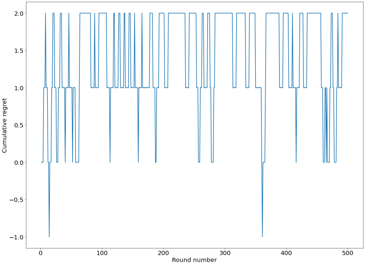
Figure 8.5: Sample cumulative regret, plotted by automate()
While we don't have any other algorithm to compare it with, from this graph, we can see that our Greedy algorithm did significantly well as it was able to keep the cumulative regret no higher than 2 at all times throughout the 500 rounds. Another way to inspect the performance of our algorithm is to consider the history list, which, again, contains the arms that the algorithm chose to pull:
print(*history)
This will print out the list in the following format:
0 1 2 0 1 2 2 2 0 0 0 0 0 0 0 0 0 0 0 0 0 0 0 0 0 0 0 0 0 0 0 0
0 0 0 0 0 0 0 0 0 0 0 0 0 0 0 0 0 0 0 0 0 0 0 0 0 0 0 0 0 0 0 0
0 0 0 0 0 0 0 0 0 0 0 0 0 0 0 0 0 0 0 0 0 0 0 0 0 0 0 0 0 0 0 0
0 0 0 0 0 0 0 0 0 0 0 0 0 0 0 0 0 0 0 0 0 0 0 0 0 0 0 0 0 0 0 0
0 0 0 0 0 0 0 0 0 0 0 0 0 0 0 0 0 0 0 0 0 0 0 0 0 0 0 0 0 0 0 0
0 0 0 0 0 0 0 0 0 0 0 0 0 0 0 0 0 0 0 0 0 0 0 0 0 0 0 0 0 0 0 0
0 0 0 0 0 0 0 0 0 0 0 0 0 0 0 0 0 0 0 0 0 0 0 0 0 0 0 0 0 0 0 0
0 0 0 0 0 0 0 0 0 0 0 0 0 0 0 0 0 0 0 0 0 0 0 0 0 0 0 0 0 0 0 0
0 0 0 0 0 0 0 0 0 0 0 0 0 0 0 0 0 0 0 0 0 0 0 0 0 0 0 0 0 0 0 0
0 0 0 0 0 0 0 0 0 0 0 0 0 0 0 0 0 0 0 0 0 0 0 0 0 0 0 0 0 0 0 0
0 0 0 0 0 0 0 0 0 0 0 0 0 0 0 0 0 0 0 0 0 0 0 0 0 0 0 0 0 0 0 0
0 0 0 0 0 0 0 0 0 0 0 0 0 0 0 0 0 0 0 0 0 0 0 0 0 0 0 0 0 0 0 0
0 0 0 0 0 0 0 0 0 0 0 0 0 0 0 0 0 0 0 0 0 0 0 0 0 0 0 0 0 0 0 0
0 0 0 0 0 0 0 0 0 0 0 0 0 0 0 0 0 0 0 0 0 0 0 0 0 0 0 0 0 0 0 0
0 0 0 0 0 0 0 0 0 0 0 0 0 0 0 0 0 0 0 0 0 0 0 0 0 0 0 0 0 0 0 0
0 0 0 0 0 0 0 0 0 0 0 0 0 0 0 0 0 0 0 0
As we can see, after the three rounds of exploration at the beginning, when it pulled each arm once, the algorithm vacillated a bit between the arms but then quickly converged to choosing arm 0, the actual optimal arm, for the rest of the rounds. This is why the resulting cumulative regret of the algorithm is so low.
With that said, this is simply one single experiment. As mentioned previously, to fully benchmark the performance of our algorithms, we need to repeat this experiments many times, making sure that the single experiment we are considering is not an outlier where the algorithm does especially well or badly due to randomness.
To facilitate repeated experiments, we utilize the repeat() method of the bandit API, as follows:
regrets = bandit.repeat(Greedy, [N_ARMS], n_experiments=100,
n_rounds=300, visualize_regret_dist=True)
Remember that the repeat() method takes in the class implementation of a given algorithm, as opposed to simply an instance of the algorithm as automate() does. This is why we are passing the whole Greedy class to the method. Additionally, with the second argument of the method, we can specify whatever arguments the class implementation of our algorithm takes in. In this case, it is simply the number of arms available to be pulled, but we will have different parameters with different algorithms in later sections.
Here, we are putting our Greedy algorithm through 100 experiments with the same bandit problem of the three Bernoulli arms we declared previously, specified by the n_experiments parameter. To save time, we only require that each experiment lasts for 300 rounds with the n_rounds parameter. Finally, we specify visualize_regret_dist to be True, which will help us plot the distribution of the cumulative regret obtained by the algorithm at the end of each experiment.
Indeed, when this code finishes running, the following plot will be produced:

Figure 8.6: Distribution of cumulative regret by the Greedy algorithm
Here, we can see that in most cases, the Greedy algorithm does sufficiently well, keeping the cumulative regret below 10. However, there are instances where the cumulative regret gets as high as 60. We speculate that these are the situations where the algorithm misestimates the true expected reward from each arm and commits too early.
As the final way to gauge how well an algorithm performs, we consider the mean and the max cumulative regret across these experiments, as follows:
np.mean(regrets), np.max(regrets)
In our current experiment, the following numbers will be printed out:
(8.66, 62)
This is consistent with the distribution that we have here: most of the regrets are low enough, causing the mean to be relatively low (8.66), but the maximum regret can get as high as 62.
And that is the end of our discussion on the Greedy algorithm. For the rest of this section, we will discuss two popular variations of the algorithm, namely Explore-then-commit and ε-Greedy.
The Explore-then-Commit Algorithm
We mentioned that a potential reason for poor performance of the Greedy algorithm in some cases is committing too early when a sufficient number of sample rewards from each arm have not been observed. The Explore-then-commit algorithm attempts to address this problem by formalizing the number of rounds that should be spent exploring each arm at the beginning of the process.
Specifically, each Explore-then-commit algorithm is parameterized by a number, T. In each bandit problem, an Explore-then-commit algorithm will spend exactly T rounds pulling each of the available arms. Only after these forced exploration rounds does the algorithm start choosing the arm with the greatest reward average. Greedy is a special case of the Explore-then-commit algorithm where T is set to 1. This general algorithm, therefore, gives us the option to customize this parameter and set it appropriately, depending on the situation.
The implementation of this algorithm is mostly similar to what we have for Greedy, so we will not consider it here. In short, instead of the conditional used to ensure the Greedy algorithm pulls each arm at least once, we can modify the conditional like so in its decide() method, given that a value for the T variable has been set:
def decide(self):
for arm_id in range(self.n_arms):
if len(self.reward_history[arm_id]) < T:
return arm_id
mean_rewards = [np.mean(history)
for history in self.reward_history]
return int(np.random.choice
(np.argwhere(mean_rewards == np.max(mean_rewards))
.flatten()))
While Explore-then-commit is a more flexible version of Greedy, it does leave open the question of how to choose the value for T. Indeed, it is not obvious how we should set T for a specific bandit problem without any prior knowledge about the problem. Most of the time, T is set with respect to the horizon if it is known beforehand; common values for T could range from 3, 5, 10, or even 20.
The ε-Greedy Algorithm
Another variation of the Greedy algorithm is the ε-Greedy algorithm. For Explore-then-commit, the amount of forced exploration depends on the settable parameter, T, which again gives rise to the question of how to best set it. For ε-Greedy, we do not explicitly require the algorithm to explore more than one round for each arm. Instead, we leave it to chance to determine when the algorithm should carry on exploitation, and when it should explore a seemingly suboptimal arm.
Formally, an ε-Greedy algorithm is parameterized by a number, ε, between zero and one, denoting the exploration probability of the algorithm. After the first exploration rounds, the algorithm will choose to pull the arm with the greatest running reward average with probability 1 - ε. Otherwise, it will uniformly choose one out of all the available arms (with probability ε). Unlike Explore-then-commit, where we know for sure the algorithm will be forced to explore for the first few rounds, an ε-Greedy algorithm might explore arms with suboptimal reward averages during later rounds too. However, when exploration happens, this is entirely due to chance, and the choice of the parameter, ε, controls how often these exploration rounds are expected to happen.
For example, a common choice for ε is 0.01. In a typical bandit problem, an ε-Greedy algorithm will pull each arm once at the start of the process and begin choosing the arm with the best reward history. However, at each step, with probability 0.01 (one percent), the algorithm might choose to explore this, in which case it will randomly choose one of all the arms without any bias. ε, like T in the Explore-then-commit algorithm, is used to control how much an MAB algorithm should explore. A high value of ε will cause the algorithm to explore more often, although, again, when it does explore, this is completely random.
The intuition behind ε-Greedy is clear: we still want to preserve the greedy nature of the Greedy algorithm, but to avoid incorrect committing to a suboptimal arm due to nonrepresentative reward samples, we also want exploration to happen every now and then throughout the entire process. Hopefully, ε-Greedy will kill two birds with one stone, being able to greedily exploit the temporarily good arms while leaving the possibility that other seemingly suboptimal arms are better open.
Implementation-wise, the decide() method of the algorithm should have an additional conditional where we check whether the algorithm should explore:
def decide(self):
...
if np.random.rand() < self.e:
return np.random.randint(0, self.n_arms)
...
And with that, let's move on and complete this chapter's first exercise, where we will implement the ε-Greedy algorithm.
Exercise 8.01 Implementing the ε-Greedy Algorithm
Similar to what we did to implement the Greedy algorithm, in this exercise, we will learn how to implement the ε-Greedy algorithm. This exercise will consist of three main sections: implementing the logic of ε-Greedy, testing it in a sample bandit problem, and finally putting it through multiple experiments to benchmark its performance.
We will follow these steps to achieve this:
- Create a new Jupyter Notebook and import NumPy, Matplotlib, and the Bandit class from the utils.py file included in the code repository for this chapter:
import numpy as np
np.random.seed(0)
import matplotlib.pyplot as plt
from utils import Bandit
Note that we are now fixing the random seed number of NumPy to ensure the reproducibility of our code.
- Now, let's begin implementing the logic of the ε-Greedy algorithm. First, its initialization method should take in two parameters: the number of arms for the bandit problem it is to solve and ε, the exploration probability:
class eGreedy:
def __init__(self, n_arms=2, e=0.01):
self.n_arms = n_arms
self.e = e
self.reward_history = [[] for _ in range(n_arms)]
Similar to what we had with Greedy, here, we are also keeping track of the reward history, which is stored in the reward_history attribute of the class object.
- In the same code cell, implement the decide() method for the eGreedy class.
This method should be mostly similar to its counterpart in the Greedy class. However, before computing the reward averages of the arms, it should draw a random number between 0 and 1 and check to see if it is less than its parameter, ε. If this is the case, it should randomly return the index of one of the arms:
def decide(self):
for arm_id in range(self.n_arms):
if len(self.reward_history[arm_id]) == 0:
return arm_id
if np.random.rand() < self.e:
return np.random.randint(0, self.n_arms)
mean_rewards = [np.mean(history)
for history in self.reward_history]
return int(np.random.choice(np.argwhere
(mean_rewards == np.max(mean_rewards))
.flatten()))
- In the same code cell, implement the update() method for the eGreedy class, which should be identical to the corresponding method in the Greedy class:
def update(self, arm_id, reward):
self.reward_history[arm_id].append(reward)
Again, this method only needs to append the most recent reward from an arm to the reward history of that arm.
And that is the complete implementation of our ε-Greedy algorithm.
- In the next code cell, create a single experiment with the bandit problem with three Bernoulli arms with respective probabilities of 0.9, 0.8, and 0.7 and run it with an instance of the eGreedy class (with ε = 0.01, which is the default value that does not need to be specified) using the automate() method.
Make sure to specify the visualize_regret=True parameter to plot out the cumulative regret of the algorithm throughout the process:
N_ARMS = 3
bandit = Bandit(optimal_arm_id=0,
n_arms=3,
reward_dists=[np.random.binomial
for _ in range(N_ARMS)],
reward_dists_params=[(1, 0.9),
(1, 0.8),
(1, 0.7)])
egreedy_policy = eGreedy(n_arms=N_ARMS)
history, rewards, optimal_rewards = bandit.automate
(egreedy_policy,
n_rounds=500,
visualize_regret=True)
This should produce the following graph:
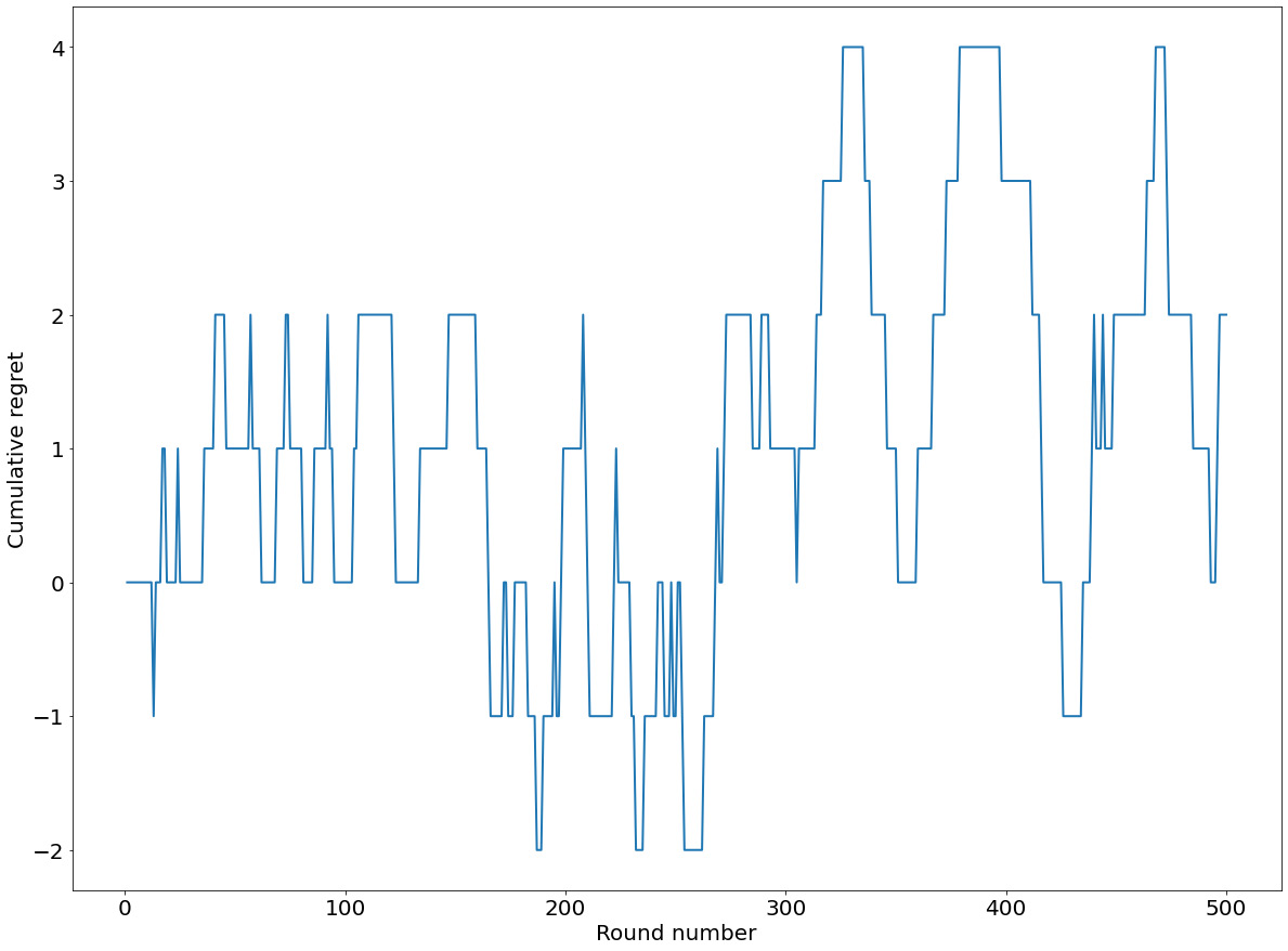
Figure 8.7: Sample cumulative regret of the ε-Greedy algorithm
Compared to the corresponding plot we saw with Greedy, our cumulative regret here has more variation, sometimes growing to 4 and sometimes dropping to -2. This is an effect of the increase in exploration of the algorithm.
- In the next code cell, we print out the history variable and see how it compares to the Greedy algorithm:
print(*history)
This will produce the following output:
0 1 2 1 2 1 0 0 1 2 1 0 0 2 0 1 1 0 0 0 0 0 0 0 0 0 0 0 0 0
0 0 0 0 0 0 0 0 0 0 0 0 0 0 0 0 0 0 0 0 0 0 0 0 0 0 0 0 0 0
0 0 0 0 0 0 0 0 0 0 0 0 0 0 0 0 0 0 0 0 0 0 0 0 0 0 0 0 0 0
0 0 0 0 0 0 0 0 0 0 0 0 0 0 0 0 0 0 0 0 0 0 0 0 0 0 0 0 0 0
0 0 0 0 0 0 0 0 0 1 0 0 0 0 0 0 0 0 0 0 0 0 0 0 0 0 0 0 0 0
0 0 0 0 0 0 0 0 0 0 0 0 0 0 0 0 0 0 0 0 0 0 0 0 0 0 0 0 0 0
0 0 0 0 0 0 0 0 0 0 0 0 0 0 0 0 0 0 0 0 0 0 0 0 0 0 0 0 0 0
0 0 0 0 0 0 0 0 0 0 0 0 0 0 0 0 0 0 0 0 0 0 0 0 0 0 0 0 0 0
0 0 1 1 1 1 1 1 0 0 0 0 0 0 0 0 0 0 0 0 0 0 0 2 0 0 0 0 0 0
0 0 0 0 0 0 0 0 0 0 0 0 0 0 0 0 0 0 0 0 0 0 0 0 1 1 0 0 0 0
0 0 0 0 0 0 0 0 0 0 0 0 0 0 0 0 0 0 0 0 0 0 0 0 0 0 0 0 0 0
0 0 0 0 0 0 0 0 0 0 0 0 0 0 0 0 0 0 0 0 0 0 0 0 0 0 0 0 0 0
0 0 0 0 0 0 0 1 0 0 0 0 0 0 0 0 0 0 0 0 0 0 0 0 0 0 0 0 0 0
0 0 0 0 0 0 1 0 0 0 0 0 0 0 0 0 0 0 0 0 0 0 0 0 0 0 0 0 0 0
0 0 0 0 0 0 0 0 0 0 0 0 0 0 0 0 0 0 0 0 0 0 0 0 0 0 0 0 0 0
0 0 0 0 0 0 0 0 0 0 0 0 0 0 0 0 0 0 0 0 0 0 0 0 0 0 0 0 0 0
0 0 0 0 0 0 0 0 0 0 0 0 0 0 0 0 0 0 0 0
Here, we can see that after the first few rounds, most of the choices made by the algorithm were all arm 0. But from time to time, arm 1 or arm 2 would be chosen, presumably from the random exploration probability.
- In the next code cell, we will conduct the same experiment, but this time, we will set ε = 0.1:
egreedy_policy_v2 = eGreedy(n_arms=N_ARMS, e=0.1)
history, rewards, optimal_rewards = bandit.automate
(egreedy_policy_v2,
n_rounds=500,
visualize_regret=True)
This will produce the following graph:
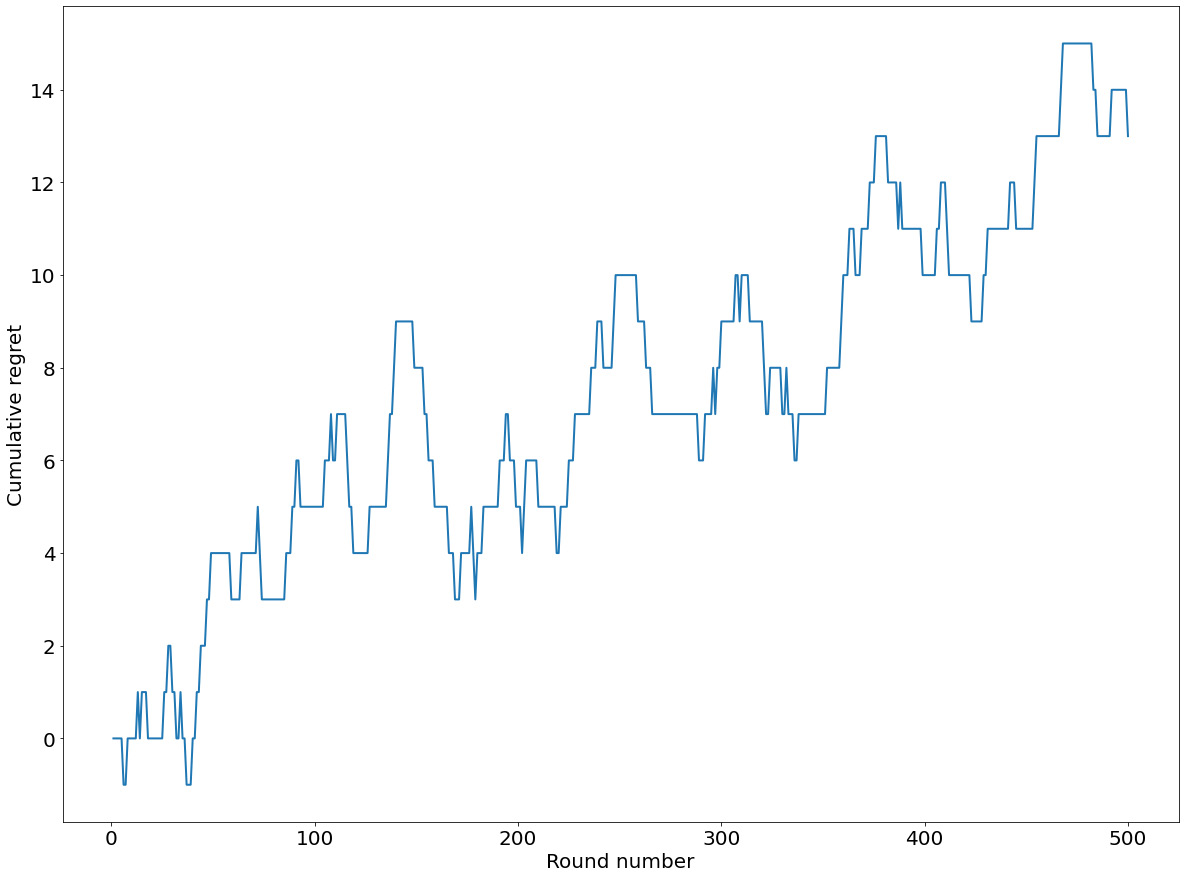
Figure 8.8: Sample cumulative regret with increased exploration probability
Here, our cumulative regret is a lot higher than what we got with ε = 0.01 in step 5. This is presumably due to the increased exploration probability, which is too high.
- To analyze this experiment further, we can print out the action history once more:
print(*history)
This will produce the following output:
0 1 2 2 0 1 0 1 2 2 0 2 2 0 2 0 0 0 0 0 0 0 0 0 0 0 0 0 0 0
0 0 0 0 0 1 0 0 0 2 0 0 0 0 0 0 0 0 0 0 0 0 0 0 0 0 0 0 0 0
0 0 0 2 0 0 0 0 0 0 0 0 0 0 0 0 0 0 0 2 0 0 0 0 0 1 2 0 1 0
0 0 0 0 0 0 0 0 2 0 0 0 0 0 0 0 0 0 0 0 0 0 0 0 0 0 0 0 0 0
0 0 0 0 0 0 0 0 0 0 0 1 2 0 0 0 0 0 1 0 0 0 1 0 0 0 0 0 0 0
0 0 0 0 0 0 0 0 0 0 0 0 0 1 0 0 0 0 0 0 0 0 0 0 0 0 0 0 2 0
0 0 0 1 0 0 0 0 0 0 0 0 0 0 0 0 0 0 0 0 0 0 0 0 0 0 0 0 0 0
0 0 0 0 0 0 0 0 0 0 0 1 0 0 0 0 0 0 0 0 0 0 0 0 0 0 0 0 1 1
0 0 0 0 0 0 2 0 0 0 1 0 0 0 0 0 0 0 0 0 0 0 0 0 0 0 0 0 2 0
0 0 0 0 0 0 0 0 0 0 0 0 0 0 0 1 0 1 0 0 0 0 0 0 0 0 0 2 0 0
0 0 0 0 0 0 0 0 0 2 0 0 0 0 0 0 0 0 0 0 0 0 0 0 0 0 0 0 0 0
0 0 0 0 0 0 0 2 2 1 0 0 0 0 0 0 0 0 0 0 0 0 0 0 0 0 0 0 0 0
0 0 2 0 0 0 0 0 0 0 0 1 0 0 0 0 0 0 0 0 0 1 0 0 0 0 0 0 0 0
0 0 0 0 0 0 0 0 0 0 0 0 0 0 0 1 0 0 0 0 0 0 0 0 0 0 0 0 0 0
0 0 0 0 0 0 0 0 0 0 0 0 0 0 0 0 1 0 0 0 0 0 0 0 0 0 0 0 0 0
0 0 0 0 0 0 0 1 0 0 0 0 0 0 0 0 0 0 2 0 0 0 2 0 0 0 0 0 0 0
0 0 0 0 1 0 0 0 0 0 0 0 0 0 0 0 0 0 0 0
Comparing this with the same history of the previous algorithm, we can see that this algorithm did indeed explore significantly more during the late rounds. All of this indicates to us that ε = 0.1 might not be an appropriate exploration probability.
- As the last component of our analysis of the ε-Greedy algorithm, let's utilize the repeated-experiment option. This time, we will choose ε = 0.03, like so:
regrets = bandit.repeat(eGreedy, [N_ARMS, 0.03],
n_experiments=100, n_rounds=300,
visualize_regret_dist=True)
The following graph will be produced, which visualizes the distribution of cumulative regret resulting from these repeated experiments:

Figure 8.9: Distribution of cumulative regret by the ε-Greedy algorithm
This distribution is quite similar to what we obtained with the Greedy algorithm. Next, we will compare the two algorithms further.
- Calculate the mean and max of these cumulative regret values with the following code:
np.mean(regrets), np.max(regrets)
The output will be as follows:
(9.95, 64)
Comparing this with what we had with the Greedy algorithm (8.66 and 62), this result indicates that the ε-Greedy algorithm might be inferior in this specific bandit problem. However, it has managed to formalize the choice between exploration and exploitation using its exploration rate, which was lacking in the Greedy algorithm. This is a valuable characteristic of a MAB algorithm, and will be the focus of other algorithms that we will be discussing in the rest of this chapter.
Note
To access the source code for this specific section, please refer to https://packt.live/3fiE3Y5.
You can also run this example online at https://packt.live/3cYT4fY.
Before we move on to the next section, let's briefly discuss yet another so-called variant of the Greedy algorithm, the Softmax algorithm.
The Softmax Algorithm
The Softmax algorithm attempts to quantify the trade-off between exploration and exploitation by choosing each of the available arms with a probability that is proportional to its average reward. Formally, the probability that arm i is chosen by the algorithm at each time step, t, is as follows:

Figure 8.10: Expression for the probability that the arm is chosen by the algorithm at each time step
Each term in the exponent ![]() is the average reward observed from arm i in the first (t - 1) time steps. Given the way the probabilities are defined, the larger this average reward is, the more likely the corresponding arm will be chosen. In its most general form, this average term is divided by a tunable parameter,
is the average reward observed from arm i in the first (t - 1) time steps. Given the way the probabilities are defined, the larger this average reward is, the more likely the corresponding arm will be chosen. In its most general form, this average term is divided by a tunable parameter, ![]() , which controls the exploration rate of the algorithm. Specifically, when
, which controls the exploration rate of the algorithm. Specifically, when ![]() tends to infinity, the probability of the largest arm will approach one while the other probabilities approach zero, making the algorithm purely greedy (which is why we consider it to be a generalization of the Greedy algorithm). The smaller
tends to infinity, the probability of the largest arm will approach one while the other probabilities approach zero, making the algorithm purely greedy (which is why we consider it to be a generalization of the Greedy algorithm). The smaller ![]() is, the more likely it is that a temporarily sub-optimal arm is chosen. As it tends to 0, the algorithm uniformly explores all the available arms indefinitely.
is, the more likely it is that a temporarily sub-optimal arm is chosen. As it tends to 0, the algorithm uniformly explores all the available arms indefinitely.
Similar to the problem we encounter while designing the ε-Greedy algorithm, it is not entirely clear how we should set the value of this parameter, ![]() , for each specific bandit problem, even though the performance of the algorithm can be highly dependent on this parameter. For that reason, the Softmax algorithm is not as popular as the algorithms we will be discussing in this chapter.
, for each specific bandit problem, even though the performance of the algorithm can be highly dependent on this parameter. For that reason, the Softmax algorithm is not as popular as the algorithms we will be discussing in this chapter.
And with that, we conclude our discussion of the Greedy algorithm, our first approach to solving the MAB problem, and three of its variations: Explore-then-commit, ε-Greedy, and Softmax. Overall, these algorithms focus on exploiting the arm with the greatest reward mean while sometimes deviating from that to explore other, seemingly suboptimal, arms.
In the next section, we will move on to another common MAB algorithm called Upper Confidence Bound (UCB), the intuition of which is slightly different from what we have seen so far.
The UCB algorithm
The term upper confidence bound denotes the fact that instead of considering the average of past rewards returned from each arm like Greedy, the algorithm computes an upper bound for its estimates of the expected reward for each arm.
This concept of a confidence bound is quite common in probability and statistics, where the distribution of a quantity that we care about (in this case, the reward from each arm) cannot be represented well using simply the average of past observations. Instead, a confidence bound is a numerical range that aims to estimate and narrow down where most of the values in the distribution in question will lie. For example, this idea is widely used in Bayesian analyses and Bayesian optimization.
In the following section, we will discuss how UCB establishes its use of a confidence bound.
Optimism in the Face of Uncertainty
Consider the middle of the process of a bandit with only two arms. We have already pulled the first arm 100 times and observed an average reward of 0.61; for the second arm, we have only seen five samples, three of which were 1, so its average reward is 0.6. Should we commit to exploring the first arm for the rest of the remaining rounds and ignore the second?
Many would say no; we should at least explore the second arm more to get a better estimation of its expected reward. The motivation for this observation is that since we only have very few samples of the reward from the second arm, we should not be confident that the mean reward of the second arm is actually lower than that of the first. How, then, should we formalize our intuition? The UCB algorithm, or specifically, its most common variant – the UCB1 algorithm – states that instead of the mean reward, we will use the following sum of the average reward and the confidence bound:

Figure 8.11: Expression for the UCB algorithm
Here, ![]() denotes the time step, or the round number, that we are currently in while interacting with a bandit, and
denotes the time step, or the round number, that we are currently in while interacting with a bandit, and ![]() denotes the number of times we have pulled arm
denotes the number of times we have pulled arm ![]() up to round
up to round ![]() . The rest of UCB works in the same way as the Greedy algorithm: at each step, we choose to pull the arm that maximizes the preceding sum, observe the returned reward, add it to our reward, and repeat the process.
. The rest of UCB works in the same way as the Greedy algorithm: at each step, we choose to pull the arm that maximizes the preceding sum, observe the returned reward, add it to our reward, and repeat the process.
To implement this logic, we can use the decide() method, which contains the following code:
def decide(self):
for arm_id in range(self.n_arms):
if len(self.reward_history[arm_id]) == 0:
return arm_id
conf_bounds = [np.mean(history)
+ np.sqrt(2 * np.log(self.t) / len(history))
for history in self.reward_history]
return int(np.random.choice
(np.argwhere(conf_bounds == np.max(conf_bounds))
.flatten()))
Here, self.t should be equal to the current step time. As we can see, the method returns the arm that maximizes the element in conf_bounds, which is the list storing the optimistic estimation of each arm.
You might be wondering why using the preceding quantity can capture the idea behind the confidence bound that we'd like to apply to our estimations of the expected reward. Remember the example of a two-arm bandit we sketched out earlier, where we would like to have a formalization that encourages exploration of the rarely explored arm (the second one, in our example). As you can see, at any given round, this quantity is a decreasing function of ![]() . In other words, the quantity gets smaller when
. In other words, the quantity gets smaller when ![]() is large and grows larger when the opposite is true. So, this quantity is maximized by the arm that has the lower number of pulls – the arm that is explored the least. In our example, the estimation of the first arm is as follows:
is large and grows larger when the opposite is true. So, this quantity is maximized by the arm that has the lower number of pulls – the arm that is explored the least. In our example, the estimation of the first arm is as follows:

Figure 8.12: Estimation of the first arm
The estimation of the second arm is as follows:

Figure 8.13: Estimation of the second arm
Using UCB, we choose to pull the second arm next, which is what we argued was the correct choice. By adding what is called an exploration term to the mean reward, we are, in a way, estimating the largest possible value of the expected mean, not just the expected mean itself. This intuition is best summed up with the term optimism in the face of uncertainty, and it is the quintessential characteristic of the UCB algorithm.
Other Properties of UCB
UCB is not unjustifiably optimistic. When an arm is significantly under-explored, the exploration term will make the sum larger, making it more likely to be chosen by UCB, but it is never guaranteed that the arm will surely be chosen. Specifically, when the mean reward of an arm is so low that a large value of the term cannot compensate for it, UCB will choose to exploit the good arms anyway.
We should also discuss its variation in cost-centric MAB problems, known as the Lower Confidence Bound (LCB). With respect to a reward-centric problem, we are adding the exploration term to the mean reward to compute an optimistic estimation of the true mean. When the MAB problem is the minimization of costs returned by the arms, our optimistic estimation becomes the mean cost subtracted by the exploration term, and the arm that minimizes this quantity will be chosen by UCB, or in this case, LCB.
In particular, we are saying that if an arm is under-explored, its true mean cost might be lower than what we have observed so far, so we subtract the average cost from the exploration term to estimate the lowest possible cost of an arm. Aside from this, the implementation of this variation of UCB remains the same.
That is enough theory about UCB. To conclude our discussions of this algorithm, we will implement it for the Bernoulli three-arm bandit problem that we have been using in the next exercise.
Exercise 8.02 Implementing the UCB Algorithm
In this exercise, we will be implementing the UCB algorithm. This exercise will walk us through the familiar workflow that we have been using to analyze the performance of an MAB algorithm: implement it as a Python class, put it through a single experiment and observe its behavior, and finally repeat the experiment many times to consider the resulting distribution of its regret.
We will follow these steps to do so:
- Create a new Jupyter Notebook and import NumPy, Matplotlib, and the Bandit class from the utils.py file included in the code repository for this chapter:
import numpy as np
np.random.seed(0)
import matplotlib.pyplot as plt
from utils import Bandit
- Declare a Python class named UCB with the following initialization method:
class UCB:
def __init__(self, n_arms=2):
self.n_arms = n_arms
self.reward_history = [[] for _ in range(n_arms)]
self.t = 0
Different from Greedy and its variants, our implementation of UCB needs to keep track of an additional piece of information, the current round number, in its attribute, t. This information is used when calculating the exploration term of the upper confidence bound.
- Implement the decide() method of the class, as follows:
def decide(self):
for arm_id in range(self.n_arms):
if len(self.reward_history[arm_id]) == 0:
return arm_id
conf_bounds = [np.mean(history)
+ np.sqrt(2 * np.log(self.t)
/ len(history))
for history in self.reward_history]
return int(np.random.choice
(np.argwhere
(conf_bounds == np.max(conf_bounds))
.flatten()))
The preceding code is self-explanatory: after pulling each arm at least once, we compute the confidence bounds as the sum of the empirical mean reward and the exploration term. Finally, we return the arm with the largest sum, randomly tie-breaking if necessary.
- In the same code cell, implement the update() method of the class, like so:
def update(self, arm_id, reward):
self.reward_history[arm_id].append(reward)
self.t += 1
We are already familiar with most of the logic here from the previous algorithms. Notice here that with each call to update(), we also need to increment the attribute, t.
- Declare the Bernoulli three-arm bandit problem that we have been considering and run it on an instance of the UCB algorithm we just implemented:
N_ARMS = 3
bandit = Bandit(optimal_arm_id=0,
n_arms=3,
reward_dists=[np.random.binomial
for _ in range(N_ARMS)],
reward_dists_params=[(1, 0.9), (1, 0.8),
(1, 0.7)])
ucb_policy = UCB(n_arms=N_ARMS)
history, rewards, optimal_rewards = bandit.automate
(ucb_policy, n_rounds=500,
visualize_regret=True)
This code will produce the following graph:

Figure 8.14: Sample cumulative regret from UCB
Here, we can see that this cumulative regret is significantly worse than what we saw with Greedy, which was, at most, 2. We hypothesize that the difference is a direct result of the optimistic nature of the algorithm.
- To understand this behavior better, we will inspect the pulling history of the algorithm:
print(*history)
This produces the following output:
0 1 2 1 0 2 0 1 1 0 1 0 2 0 2 0 0 1 0 1 0 1 0 1 2 0 1 0 1 0 0
1 0 1 0 1 0 0 0 2 2 1 1 0 1 0 1 0 1 0 1 1 1 2 2 2 2 0 2 0 2 0
1 1 1 1 1 0 0 0 0 0 2 2 0 0 1 0 1 0 0 0 0 0 1 0 2 2 2 0 0 0 0
0 0 0 0 1 0 1 0 1 1 0 1 0 1 0 1 0 0 0 0 2 2 2 0 0 0 0 0 0 0 0
0 1 1 0 1 0 0 0 0 0 0 2 2 2 2 2 0 1 0 1 1 0 1 0 0 0 0 0 0 2 2
2 2 0 0 1 0 1 1 0 1 0 0 0 0 0 0 0 0 0 1 0 1 1 1 0 2 1 1 0 1 0
1 1 1 1 1 1 1 0 0 0 0 0 0 1 1 1 0 0 2 2 2 0 0 0 1 1 1 0 0 0 0
0 0 2 2 0 0 0 0 0 1 0 0 0 0 0 0 0 0 0 0 0 0 0 0 1 1 1 0 0 0 0
0 0 0 0 0 0 2 2 2 2 2 2 2 2 0 0 0 0 0 0 2 2 2 2 1 1 1 1 1 1 0
0 0 0 0 0 1 1 1 1 1 1 1 1 1 2 2 2 2 0 0 0 0 0 0 1 1 0 0 0 0 0
0 0 0 0 0 0 0 0 0 0 0 0 0 0 0 2 2 0 0 0 0 0 0 0 0 0 0 0 0 0 1
1 1 1 0 0 0 0 0 0 0 0 0 0 0 0 0 0 0 0 0 2 2 1 0 0 0 0 0 0 0 0
0 0 0 0 0 0 0 0 0 0 0 1 1 1 1 0 2 2 0 0 0 0 0 0 0 0 0 0 0 0 1
1 1 1 0 0 0 0 0 0 0 0 0 0 0 0 0 0 0 0 0 0 0 0 0 0 0 0 0 2 1 1
1 0 0 0 0 0 0 0 0 1 1 1 1 0 0 0 0 0 0 0 0 2 2 2 2 2 2 2 0 0 0
0 0 0 0 0 0 0 0 0 0 1 1 1 1 1 1 1 1 1 0 0 0 2 2 2 2 2 0 0 1 1 0 0 0 0
Here, we can observe that instead of exploiting the true optimal arm (arm 0), UCB frequently chose to deviate. This is a direct effect of its tendency to optimistically explore seemingly suboptimal arms.
- At face value, we might conclude that for this bandit problem, UCB is, in fact, not superior than the Greedy algorithm, but to truly confirm whether that is true or not, we need to inspect how the algorithm does across multiple experiments. Use the repeat() method from the bandit API to confirm this:
regrets = bandit.repeat(UCB, [N_ARMS], n_experiments=100,
n_rounds=300, visualize_regret_dist=True)
This code snippet will generate the following plot:

Figure 8.15: Distribution of regret of UCB
To our surprise, the regret values in this distribution are significantly lower than those resulting from the Greedy algorithm.
- In addition to visualizing the distribution, we also need to consider the average and max regret across all experiments:
np.mean(regrets), np.max(regrets)
The output will be as follows:
(18.78, 29)
As you can see, the values are significantly lower than the corresponding statistics we saw in Greedy, which were 8.66 and 62. Here, we can say that we have evidence supporting the claim that UCB is better than Greedy in terms of minimizing the cumulative regret of a bandit problem.
Note
To access the source code for this specific section, please refer to https://packt.live/3fhxSmX.
You can also run this example online at https://packt.live/2XXuJmK.
This example also illustrates the importance of repeating experiments when analyzing the performance of a MAB algorithm. As we saw earlier, using just a single experiment, we could have arrived at the wrong conclusion that UCB is inferior to the Greedy algorithm in the specific bandit problem we are considering. However, across many repeated experiments, we can see that the opposite is true.
Throughout this exercise, we have implemented UCB, as well as learned about the need for comprehensive analysis with multiple experiments while working with MAB algorithms. This also marks the end of the topic surrounding the UCB algorithm. In the next section, we will begin talking about the last MAB algorithm in this chapter: Thompson Sampling.
Thompson Sampling
The algorithms we have seen so far make up a set of diverse insights: Greedy and its variants mostly focus on exploitation and might need to be explicitly forced to employ exploration; UCB, on the other hand, tends to be optimistic about the true expected reward of under-explored arms and therefore naturally, but also justifiably, focuses on exploration.
Thompson Sampling also uses a completely different intuition. However, before we can understand the idea behind the algorithm, we need to discuss one of its principal building blocks: the concept of Bayesian probability.
Introduction to Bayesian Probability
Generally speaking, the workflow of using Bayesian probability to describe a quantity consists of the following elements:
- A prior probability representing whatever prior knowledge or belief we have about the quantity.
- A likelihood probability that denotes, as the name of the term suggests, how likely the data that we have observed so far is.
- And finally, a posterior probability, which is the combination of the preceding two elements.
One fundamental component of Bayesian probability is Bayes' theorem:

Figure 8.16: Bayes' theorem
Here, P(X) denotes the probability of a given event, X, while P(X | Y) is the probability of a given event, X, provided that event Y has already happened. The latter is an example of conditional probabilities, which is a common object in machine learning, especially when different events/quantities are conditionally dependent on each other.
This specific formula outlines the general idea of Bayesian probability that we have here: say we are given a prior probability for an event, A, and we also know how likely event B happens given event A. Here, the posterior probability of the same event, A, given event B, is proportional to the product of the two aforementioned probabilities. Event A is typically what we care about, while event B is the data that we have observed. To put this into perspective, let's consider the application of this formula in the context of a Bernoulli distribution.
We'd like to estimate the unknown parameter, p, that characterizes a Bernoulli distribution, from which we have observed five samples. Due to how a Bernoulli distribution is defined, the probability that the sum of these five samples is equal to x, an integer between 0 and 5, is ![]() (don't worry if you aren't familiar with this expression).
(don't worry if you aren't familiar with this expression).
But what if the samples are what we can observe, and we are unsure what the actual value of p is? How can we "flip" the direction of the preceding probabilistic quantity so that we can draw some conclusions about the value of p from the samples? This is where Bayes' theorem comes into play. In the Bernoulli example, from the likelihood of the sum of the observed samples given any value of p, we can calculate the probability that p is indeed that value, given the observations that we have.
This is directly connected to the MAB problem. We, of course, always start out not knowing what the actual value, p, that parameterizes the reward distribution of a given arm is, but we can observe the reward samples drawn from it by pulling that arm. So, from a number of samples, we can calculate what the probability that p is equal to, say, 0.5 is, and whether that probability is larger than the probability that p is equal to 0.6.
A question remains about how to choose the prior distribution for p. In our case, when we start out without any prior information about p, we might say that p is equally likely to be any number between 0 and 1. So, we model p using a uniform distribution between 0 and 1. The Beta distribution is a generalization of the uniform distribution where its parameters are α = 1 and β = 1, so let's say p, for now, follows Beta(1, 1).
Bayes' theorem allows us to update this Beta distribution to another Beta distribution with different parameters after seeing some observations. Following our running example, say, after five separate observations from this Bernoulli distribution that we are modeling, we have three instances of 1 and two instances of 0. According to the Bayesian updating rule (the math of which is out of scope for this book), a Beta distribution with α and β parameters will be updated to α + 3 and β + 2.
Note
In general, out of n observations, x of which are 1 and the others are 0, a Beta(α, β) distribution will be updated to Beta(α + x, β + n - x). Roughly speaking, in an update, α should be incremented by the number of samples observed, while β should be incremented by the number of zero samples.
From this newly updated distribution, which reflects that data that we can observe, the new estimation of p, which is the mean of the distribution, can be computed as α / (α + β). We said that we typically start out by modeling p using a uniform, or Beta(1, 1), distribution; the expectation of p, in this case, is 1 / (1 + 1) = 0.5. As we see more and more samples from the Bernoulli distribution with the true value of p, we will update this Beta distribution that we are using to better model p to reflect which values of p are now likely, given those samples.
Let's consider a visual illustration to tie all of this together. Consider a Bernoulli distribution with p = 0.9, which we consider unknown to us. We can, again, only draw samples from this distribution and we'd like to use the Bayesian update rule described previously to model our belief about p. Say that at each timestep out of 1,000 timesteps, we can draw one sample from the distribution. Our observations are as follows:
- At timestep 0, we don't have any observations yet.
- At timestep 5, we have all observations being ones, and none being zero.
- At timestep 10, we have 9 positive observations and 1 zero.
- At timestep 20, we have 18 positive observations and 2 zeros.
- At timestep 100, we have 91 positive observations and 9 zeros.
- At timestep 1,000, we have 892 positive observations and 108 zeros.
First of all, we can see that the fraction of positive observations is roughly equal to the true value of p = 0.9, which is unknown to us. Additionally, we don't have any prior knowledge on this value of p, so we choose to model it using Beta(1, 1). This corresponds to the horizontal probability density function that we have in the upper-left panel of the following plot.
For the rest of the panels, we use the Bayesian update rule to compute a Beta distribution with new parameters to fit the data we observe better. The blue lines are the probability density function of p, indicating how likely it is that p is equal to one specific value between 0 and 1, given the observations we have.
At timestep 5, all of our observations are one, so our belief gets update to reflect that the probability that p is some value close to 1 is very large. This is indicated by an increase in probability mass on the right-hand side of the plot. At timestep 10, one zero observation occurs, so the probability that p is exactly 1 decreases, giving more mass to the values close to but below 1. In latter timesteps, the curve grows tighter and tighter, indicating that the model is becoming more and more confident about what values p can take on. Finally, at timestep 1,000, the function peaks around the point 0.9 and nowhere else, indicating that it is extremely confident p is roughly 0.9:
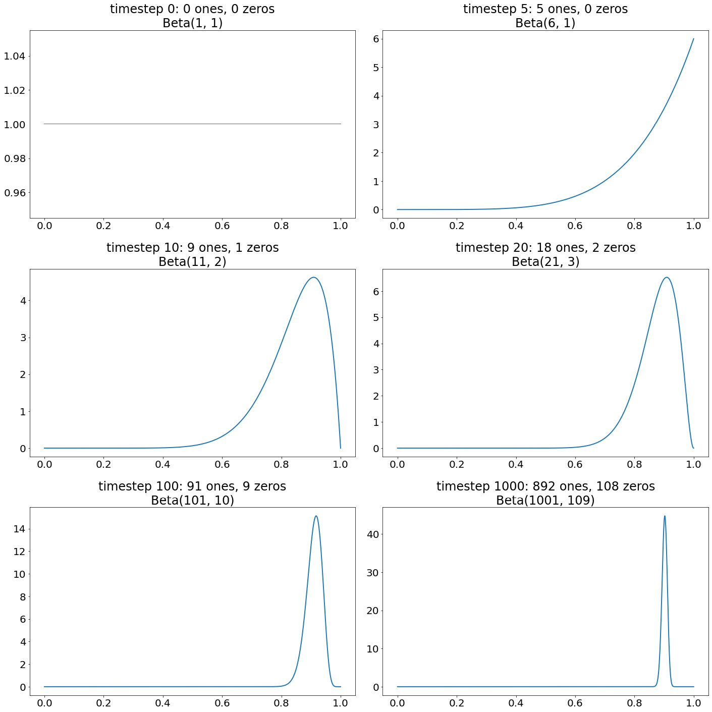
Figure 8.17: A visual illustration of the Bayesian updating process
In our example, Beta distributions are used to model the unknown parameter of a Bernoulli distribution; it is important that Beta distributions are used because when Bayes' theorem is applied, the prior probability associated with a Beta distribution, combined with the likelihood probability of a Bernoulli distribution, simplifies the math significantly, allowing the posterior to become a different Beta distribution with newly updated parameters. If another distribution aside from Beta were to be used, the formula would not be simplified in such a way. The Beta distribution is therefore called the conjugate prior of the Bernoulli distribution. In Bayesian probability, when we'd like to model the unknown parameters of a given distribution, the conjugate prior of that distribution should be used so that the math will work out.
If this process is still confusing to you, don't worry, as most of the theory behind Bayesian updating and conjugate priors has already been worked out for common probability distributions. For our purposes, we simply need to remember the update rule for the Bernoulli/Beta distribution that we just discussed.
Note
For those of you who are interested, please feel free to consult the following material from MIT, which further introduces conjugate priors of various probability distributions: https://ocw.mit.edu/courses/mathematics/18-05-introduction-to-probability-and-statistics-spring-2014/readings/MIT18_05S14_Reading15a.pdf.
So far, we have learned how to model the unknown parameter, p, of a Bernoulli distribution in a Bayesian fashion when given data that we can observe. In the next section, we will finally connect this topic back to our original point of discussion: the Thompson Sampling algorithm.
The Thompson Sampling Algorithm
Consider the Bayesian technique of modeling p that we just learned about in the context of an MAB problem with Bernoulli reward distributions. We now have a way to quantify, probabilistically, our belief about the value of p, given the reward samples we have observed from the corresponding arm. From here, we can simply employ a greedy strategy again and choose the arm with the greatest expectation of p, which is, again, computed as α / (α + β), where α and β are the running parameters of the current Beta distribution modeling p.
Instead, to implement Thompson Sampling, we draw a sample from each of the Beta distributions that model the p parameter of each of the Bernoulli distributions and select the maximal one. In other words, each arm in the bandit problem has a Bernoulli reward distribution whose parameter, p, is being modeled by some Beta distribution. We sample from each of these Beta distributions and pick the arm with the highest-valued sample.
Let's say that, in the class object syntax that we have been using to implement MAB algorithms, we store the running values of alpha and beta used by a Beta distribution in the temp_beliefs attribute to model the parameter, p, of each arm. The logic of Thompson Sampling can be applied as follows:
def decide(self):
for arm_id in range(self.n_arms):
if len(self.reward_history[arm_id]) == 0:
return arm_id
draws = [np.random.beta(alpha, beta, size=1)
for alpha, beta in self.temp_beliefs]
return int(np.random.choice
(np.argwhere(draws == np.max(draws)).flatten()))
Different from Greedy or UCB, to estimate the true value of p for each arm, we draw a random sample from the corresponding Beta distribution whose parameters have been updated by the Bayesian updating rule throughout the process (as can be seen in the draws variable). To choose an arm to pull, we simply identify the arm that has the best sample.
Two immediate questions come to mind: first, why is this sampling process a good way to estimate the reward expectation of each arm, and second, how does the technique address the trade-off between exploration and exploitation?
When we sample from each of the Beta distributions, the more likely p is equal to a given value, the more likely that value will be chosen as our sample – this is simply the nature of a probability distribution. So, in a way, a sample from a distribution is an approximation of the quantity that the distribution models. This is why samples from the Beta distributions can be justifiably used as estimations of the true value of p of each of the Bernoulli distributions.
With that said, when the current distribution representing our belief about parameter p of a given Bernoulli is flat and does not have a sharp peak (as opposed to the one in the final panel of the preceding visualization), it indicates that we still have a lot of uncertainty about what value p might be, which is why many numbers are given more probability mass than in a distribution with a single sharp peak. When a distribution is relatively flat, the samples drawn from it are likely to be dispersed across the range of the distribution, as opposed to surrounding one single region, again indicating our uncertainty about the true value. All of this is to say that even though samples can be used as approximations of a given quantity, the accuracy of those approximations depends on how flat the modeling distribution is (and therefore, ultimately, how certain our belief is about the true value).
This fact directly helps us address the exploration-exploitation dilemma. When samples for p's are drawn from distributions with single sharp peaks, they are more likely to be very close to the true values of the corresponding p's, so choosing the arm with the highest sample is equivalent to choosing the arm with the highest p (or expected reward). When a distribution is still flat, the values of the samples drawn from it are likely to be volatile and might, therefore, take on large values. If, somehow, an arm is chosen because of this reason, this means that we are not certain enough about the value of p for this arm, and it's therefore worth exploring.
Thompson Sampling, by sampling from the modeling distributions, offers an elegant method of balancing exploitation and exploration: if we are certain with our beliefs about each arm, picking the best sample is likely to be equivalent to picking the actual optimal arm; if we are not certain about an arm enough that its corresponding sample has the best value, exploring it will be beneficial.
As we will see in the upcoming exercise, the actual implementation of Thompson Sampling is quite straightforward, and we won't need to include much of the theoretical Bayesian probability that we have discussed in the implementation.
Exercise 8.03: Implementing the Thompson Sampling Algorithm
In this exercise, we will be implementing the Thompson Sampling algorithm. As always, we will be implementing the algorithm as a Python class and subsequently applying it to the Bernoulli three-arm bandit problem. Specifically, we will walk through the following steps:
- Create a new Jupyter Notebook and import NumPy, Matplotlib, and the Bandit class from the utils.py file included in the code repository for this chapter:
import numpy as np
np.random.seed(0)
import matplotlib.pyplot as plt
from utils import Bandit
- Declare a Python class named BernoulliThompsonSampling (indicating that the class will be implementing the Bayesian update rule for Bernoulli/Beta distributions) with the following initialization method:
class BernoulliThompsonSampling:
def __init__(self, n_arms=2):
self.n_arms = n_arms
self.reward_history = [[] for _ in range(n_arms)]
self.temp_beliefs = [(1, 1) for _ in range(n_arms)]
Remember that in Thompson Sampling, we maintain a running belief about p of each Bernoulli arm using a Beta distribution whose two parameters are updated according to the update rule. Therefore, we only need to keep track of the running values of these parameters; the temp_beliefs attribute contains this information for each of the arms, whose default value is (1, 1).
- Implement the decide() method, using the np.random.beta function from NumPy to draw a sample from a Beta distribution, like so:
def decide(self):
for arm_id in range(self.n_arms):
if len(self.reward_history[arm_id]) == 0:
return arm_id
draws = [np.random.beta(alpha, beta, size=1)
for alpha, beta in self.temp_beliefs]
return int(np.random.choice
(np.argwhere(draws == np.max(draws)).flatten()))
Here, we can see that instead of computing the mean reward or its upper confidence bound, we simply draw a sample from each of the Beta distributions defined by the parameters stored in the temp_beliefs attribute.
Finally, we pick the arm that corresponds to the maximum sample.
- In the same code cell, implement the update() method for the class. In addition to appending the most recent reward to the history of the appropriate arm, we need to implement the logic of the update rule:
def update(self, arm_id, reward):
self.reward_history[arm_id].append(int(reward))
# Update parameters according to Bayes rule
alpha, beta = self.temp_beliefs[arm_id]
alpha += reward
beta += 1 - reward
self.temp_beliefs[arm_id] = alpha, beta
Remember that the first parameter, α, should be incremented once for every sample we observe, while β should be incremented if the sample is zero. The preceding code implements this logic.
- Next, set up the familiar Bernoulli three-arm bandit problem and apply an instance of the Thompson Sampling class implementation to it to plot out the cumulative regret in that single experiment:
N_ARMS = 3
bandit = Bandit(optimal_arm_id=0,
n_arms=3,
reward_dists=[np.random.binomial
for _ in range(N_ARMS)],
reward_dists_params=[(1, 0.9), (1, 0.8),
(1, 0.7)])
ths_policy = BernoulliThompsonSampling(n_arms=N_ARMS)
history, rewards, optimal_rewards = bandit.automate
(ths_policy, n_rounds=500,
visualize_regret=True)
The following graph will be produced:

Figure 8.18: Sample cumulative regret from Thompson Sampling
This regret plot is better than the one we obtained with UCB but worse than the one from Greedy. The plot will be used in conjunction with the pulling history in the next step for further analysis. Let's analyze the pulling history further.
- Print out the pulling history:
print(*history)
The output will be as follows:
0 1 2 0 0 2 0 0 0 1 0 2 2 0 0 0 2 0 2 2 0 0 0 2 2 0 0 0 0 0 0
0 0 0 0 0 2 2 0 0 0 0 0 0 0 0 0 0 1 0 0 0 0 0 0 0 0 0 0 0 0 1
0 1 2 0 0 0 0 0 0 2 0 0 0 0 0 0 0 0 0 1 0 1 0 1 0 0 2 1 1 0 2
0 1 0 0 0 0 0 0 0 0 0 0 0 0 0 0 2 0 0 0 0 0 0 0 0 1 1 0 0 0 1
0 0 0 0 0 0 0 0 0 0 0 2 0 0 0 1 0 0 0 0 0 0 0 0 0 0 1 0 0 0 0
0 0 0 0 0 0 0 0 0 0 0 1 0 0 0 0 0 0 0 2 0 0 0 0 0 0 0 0 0 0 0
0 0 0 0 0 0 0 0 0 0 0 1 2 0 0 0 0 0 0 0 0 0 0 2 0 0 0 0 0 0 0
0 0 0 0 0 0 1 0 0 0 0 0 0 0 0 0 0 0 0 0 0 0 0 0 0 0 0 0 0 0 0
0 0 0 0 0 0 0 0 0 0 0 0 0 0 0 0 0 0 0 0 0 0 0 0 0 0 0 0 0 0 0
0 0 0 2 1 0 0 0 0 0 0 0 2 0 0 0 0 0 0 2 0 0 0 0 0 0 0 0 2 0 2
0 0 0 0 0 0 0 2 2 0 0 0 0 0 0 2 0 0 0 0 0 0 0 0 0 0 0 0 0 2 0
0 0 0 0 0 0 0 0 0 0 0 0 0 0 0 0 0 0 0 0 0 0 0 0 0 0 0 0 0 1 0
0 0 1 0 0 0 0 1 0 0 0 0 0 0 0 0 0 0 0 0 0 0 0 0 0 0 0 0 0 0 0
0 0 0 0 0 0 0 0 0 0 0 0 0 0 0 0 0 0 0 1 0 0 0 0 0 0 0 0 0 0 0
0 0 0 0 2 0 0 2 0 0 0 0 0 0 0 1 0 0 0 0 0 0 0 0 0 0 0 0 0 0 0
1 0 0 0 0 0 0 0 0 0 0 0 0 0 0 0 0 0 0 0 2 0 0 0 0 0 0 0 0 0 0 0 0 0 0
As you can see, the algorithm was able to identify the optimal arm but deviated to arms 1 and 2 from time to time. However, the exploration frequency decreased as time went on, indicating that the algorithm was growing more and more certain about its beliefs (in other words, each running Beta distribution was consolidating around a single peak). This is the typical behavior of Thompson Sampling.
- As we have learned, just considering one single experiment might not be sufficient for the analysis of an algorithm. To facilitate a fuller analysis on the performance of Thompson Sampling, let's set up the usual repeated experiments:
regrets = bandit.repeat(BernoulliThompsonSampling, [N_ARMS],
n_experiments=100, n_rounds=300,
visualize_regret_dist=True)
This will generate the following distribution of regret:
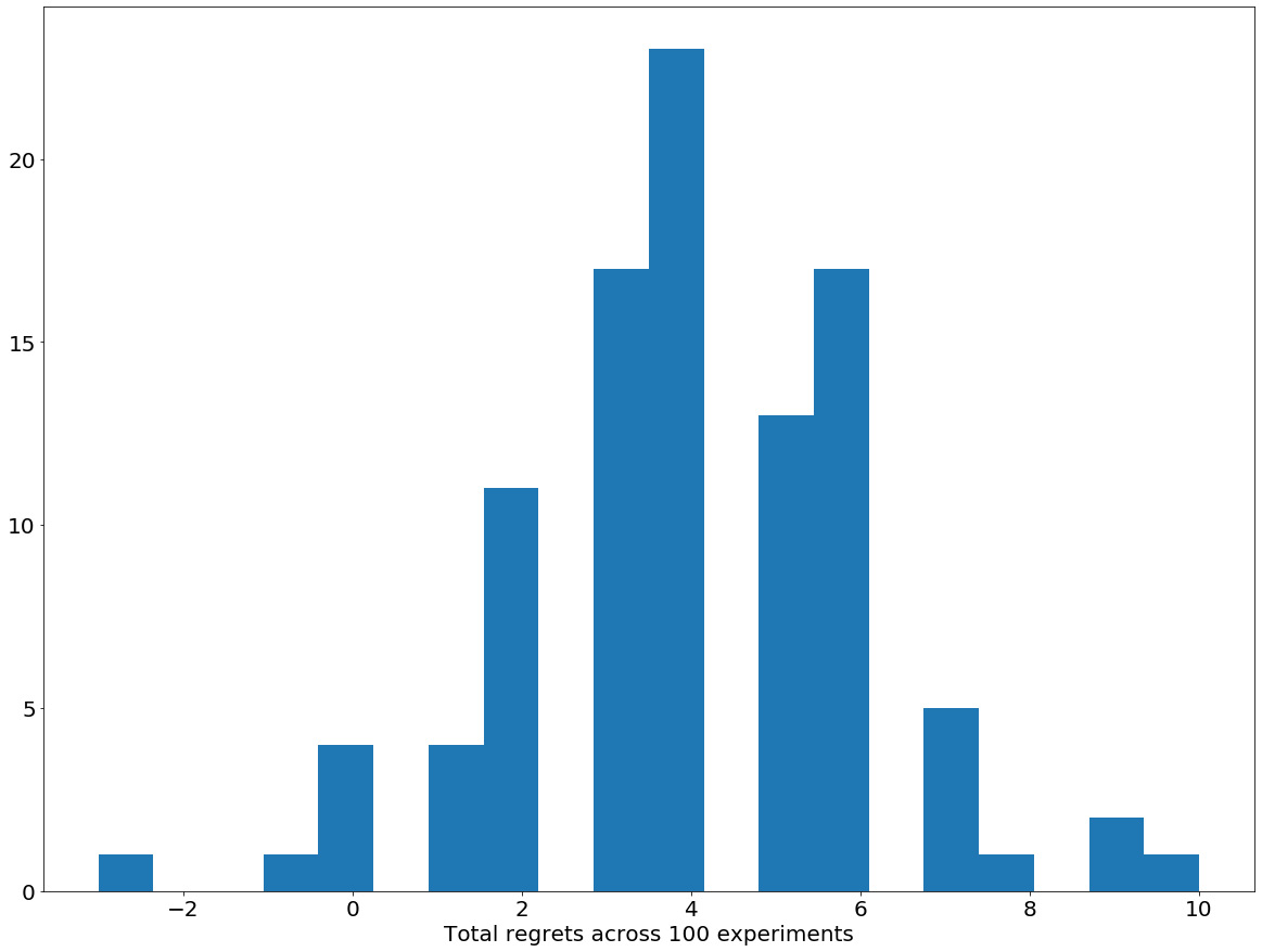
Figure 8.19: Distribution of cumulative regret from Thompson Sampling
Here, we can see that Thompson Sampling is able to minimize the cumulative regret across all experiments by a large margin compared to other algorithms (the maximum value in the distribution is only 10).
- To quantify this claim, let's print out the mean and max regret from these experiments:
np.mean(regrets), np.max(regrets)
The output will be as follows:
(4.03, 10)
This is significantly better than the counterpart statistics from other algorithms: Greedy had 8.66 and 62 while UCB had 18.78 had 29.
Note
To access the source code for this specific section, please refer to https://packt.live/2UCbZXw.
You can also run this example online at https://packt.live/37oQrTz.
Thompson Sampling is also the last of the common MAB algorithms that will be discussed in this book. In the next and final section of this chapter, we will briefly consider a common variant of the classical MAB problem, namely the contextual bandit problem.
Contextual Bandits
In the classical bandit problem, the reward from pulling an arm solely depends on the reward distribution associated with that arm, and our goal is to identify the optimal arm as soon as possible and keep pulling it until the end of the process. A contextual bandit problem, on the other hand, includes an additional element to the problem: the environment, or the context. Similar to its definition in the context of reinforcement learning, an environment contains all of the information about the problem settings, the state of the world at any given time, as well as other agents that might be participating in the same environment as our player.
Context That Defines a Bandit Problem
In the traditional MAB problem, we only care about what potential reward each arm will return if we pull it at any time. In contextual bandits, we are provided with the contextual information about the environment that we are operating in, and depending on the setting, the reward distribution of an arm might vary. In other words, the choice of which arm to pull that we make at every step should be dependent on the state of the environment, or the context.
This setting complicates the model that we have been working with, as now, we will need to consider the quantities that we are interested in as conditional probabilities: given the context we are seeing, what is the probability that arm 0 is the optimal arm, for example? In a contextual bandit problem, the context might have a minor role in the decision process of our algorithms, or it could be the main factor that drives the algorithm's decisions.
A real-world example is in order. We mentioned at the beginning of this chapter that recommender systems are a common application of the MAB problem, where, for each user who has just arrived at a website, the system needs to decide which kind of ads/recommendations would maximize the probability that the user would be interested in it. Every user has their own preferences and liking, and those factors might very well play an important role in helping the system decide whether they will be interested in a specific ad or not.
For example, dog owners will be significantly more likely to click on dog toy advertisements than the average user and potentially less likely to click on cat food advertisements. This information about the users is a part of the context of the MAB problem, which is the current recommender system we are considering. Other factors might include their profiles, buying/viewing history, and so on.
Overall, in a contextual bandit problem, we need to consider the expectation of reward of each arm/decision and do so while keeping the current context that we are in in mind. Now, let's start talking about the contextual bandit problem that we will be solving in the upcoming activity; it is also a problem that we have mentioned a couple of times throughout this book: queueing bandits.
Queueing Bandits
Our bandit problem has the following elements:
- We start out with a queue of customers, each of whom belongs to one of a predetermined set of customer classes. For example, let's say our queueing contains 300 customers in total. Among these customers, 100 customers belong to class 0, another 100 belong to class 1, and the other 100 belong to class 2.
- We also have a single server that is to serve all of these customers in a specific order. Only one customer can be served at any given time, and when a customer is being served, the remaining ones in the queue will have to wait until it is their turn to be served. Once a customer has been served, they leave the queue completely.
- Each customer has a specific job length, that is, the amount of time that it will take for the server to begin and end the customer's service. The job length of a customer belonging to class i (i is 0, 1, or 2) is a random sample drawn from an exponential distribution with parameter λi, called the rate parameter. The larger the parameter is, the more likely it is that a sample drawn from the distribution is small. In other words, the expected value of a sample is inversely proportional to the rate parameter. (In fact, the mean of an exponential distribution is 1, divided by its rate parameter.)
Note
If you are interested in learning more about the exponential distribution, you can find more information here: https://mathworld.wolfram.com/ExponentialDistribution.html. For our purposes, we only need to know that the expected value of an exponentially distribution random variable is inversely proportional to the rate parameter.
- When a customer is being served, all the customers remaining in the queue will contribute to the total cumulative waiting time that we will incur at the end of the process. Our goal, as the queue coordinator, is to come up with a way of ordering these customers so that the total cumulative waiting time of all of the customers at the end of the process is minimized. It is known that the optimal ordering to minimize this total cumulative waiting time is shortest job first, where out of the remaining customers at any given time, the one with the shortest job length should be chosen.
With this, we can see the parallel between this queueing problem and the classical MAB problem. If the true rate parameter that characterizes the job length distribution of customers belonging to a given class is not known, we need to find a way to estimate that quantity by observing the job length of a few sample customers from each class. The sooner we can identify and converge on processing the customers with the highest rate parameter, the lower our total cumulative waiting time at the end will be. Here, pulling an arm is equivalent to picking a customer of a given class to serve next, and the negative reward (or cost) that we need to minimize at the end is the cumulative waiting time of the whole queue.
As a contextual bandit problem, a queueing problem also contains some extra context at each step that needs to be considered in the decision-making process. For example, we mentioned that in each experiment, we start out with a queue of finitely many customers (specifically, 100 customers for each of three different classes), and once a customer is processed, they will leave the queue forever. This means each of the three "arms" of our bandit problem has to be pulled exactly 100 times, and an algorithm needs to find a way to arrange the order of these pulls optimally.
In the next section, the API for the queueing bandit problem we have provided for you will be discussed.
Working with the Queueing API
To have the problem defined via an API, make sure to download the two following files from the code repository for this chapter, utils.py, which contains the API for traditional bandit problems that we have been using, as well as queueing bandit problems, and data.csv, which includes the input data that will be used for our queueing experiments.
Now, different from the API that we have been using, we need to do the following to interact with a queueing bandit. First, from the utils.py file, the QueueBandit class needs to be imported. An instance of this class is declared like so:
queue_bandit = QueueBandit(filename='../data.csv')
The filename argument takes in the relative location of your code and the data.csv file, so that might change, depending on where your own notebook is. Unlike the Bandit class, because the data.csv file contains data generated from multiple experiments with different randomly chosen parameters, we don't need to declare those specific details ourselves. In fact, what we mentioned previously applies to all experiments that we will be using: in each experiment, we have the input of a 300-customer queue belonging to three different customer classes with varying unknown rate parameters.
This API also offers us the repeat() method so that we have an algorithm interact with the queueing problem, which similarly takes in a class implementation of that algorithm and any potential parameters as its two main arguments. The method will run the input algorithm through many different starting queues (which, again, were generated with different rate parameters for the three classes) and return the cumulative waiting time for each of those queues. The method also has an argument named visualize_cumulative_times, which, if set to True, will visualize the distribution of that cumulative waiting time in a histogram.
A call to this method should look as follows:
cumulative_times = queue_bandit.repeat
([ALG NAME], [ANY ALG ARGUMENTS],
visualize_cumulative_times=True)
Finally, the last difference that we need to keep in mind is the requirement for algorithm implementations. The class implementation of an algorithm should have an update() method that acts the same way as we have become familiar with (it should take in the index of an arm (or of a customer class) and the most recent corresponding cost (or job length) and update whatever appropriate information that the algorithm keeps track of).
More importantly, the decide() method should now take in an argument that indicates how many customers of each class we have left in the queue at any given time, stored in a three-item Python list. Remember that we always start out with a queue consisting of 100 customers for each class, so the list at the beginning will be [100, 100, 100]. As customers are chosen by our algorithms and served, this list of customer numbers will be updated accordingly. This is the context that our algorithm needs to keep in mind while making its decisions; obviously, it cannot choose to serve a customer from class 1 next, for example, if there is no class-1 customer left in the queue. Finally, the decide() method should return the index of the class that should be chosen to serve, similar to what we had with the traditional MAB problem.
And that is what we need to know about this queueing bandit problem. While marking the end of the materials covered in this chapter, this section also prepares us for the upcoming activity: implementing various algorithms to solve the queueing bandit problem.
Activity 8.01: Queueing Bandits
As mentioned previously, a queueing problem where the true rate parameters of the customer job lengths are unknown can be framed as a MAB problem. In this activity, we will be reimplementing the algorithms that we have learned about in this chapter in the context of queueing and comparing their performance. This activity will, therefore, reinforce the concepts that we have discussed throughout this chapter, while giving us the opportunity to tackle a contextual bandit problem.
With that, let's start the activity by following these steps:
- Create a new Jupyter Notebook and in its first code cell, import NumPy and the QueueBandit class from utils.py. Be sure to set the random seed of NumPy to 0.
- Declare an instance of this class using the code included in the preceding text.
- In a new code cell, implement the Greedy algorithm for this queueing problem and apply it to the bandit object using the code included in the preceding text. Along with the histogram of the cumulative waiting time distribution, print out the mean and max items among them.
Again, the Greedy algorithm should choose the customer class that has the lower average job length out of the remaining classes at each iteration of a queue.
The output will be as follows:

Figure 8.20: Distribution of cumulative waiting time from Greedy
The max and mean cumulative waiting times will be as follows:
(1218887.7924350922, 45155.236786598274)
- In a new code cell, implement the Explore-then-commit algorithm for the problem. The class implementation of the algorithm should take in a parameter named T that specifies how may exploration rounds the algorithm should take in at the beginning of an experiment.
- Similar to the Greedy algorithm, apply Explore-then-commit with T=2 to the bandit object. Compare the distribution of the cumulative waiting times, as well as the mean and max resulting from this algorithm, with what we have for Greedy.
This will produce the following graph:
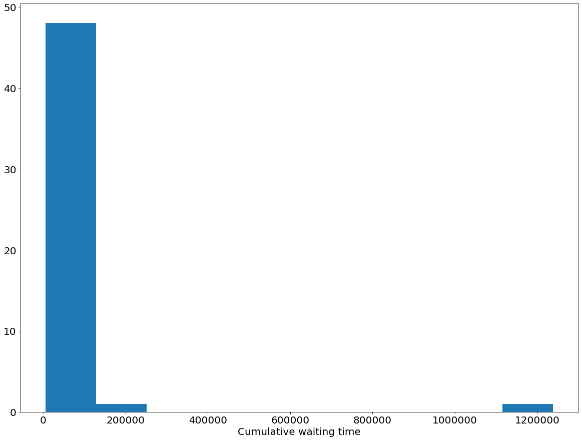
Figure 8.21: Distribution of cumulative waiting time from Explore-then-commit
The max and mean cumulative waiting times will be as follows:
(1238591.3208636027, 45909.77140562623)
- In a new code cell, implement the Thompson Sampling algorithm for the problem.
To model an unknown rate parameter of an exponential distribution, a Gamma distribution should be used as the conjugate prior. A Gamma distribution is also parameterized by two numbers, α and β; their update rule with respect to a sample job length, x, is α = α + 1 and β = β + x. At the beginning, both parameters should be initialized to 0.
To draw a sample from a Gamma distribution, the np.random.gamma() function could be used, which takes in α and 1 / β. Similar to our logic for Greedy and Explore-then-commit, the class with the highest sampled rate should be chosen at each iteration.
- Apply the algorithm to the bandit object and analyze its performance via the cumulative waiting times. Compare it to Greedy and Explore-then-commit.
The following plot will be produced:

Figure 8.22: Distribution of cumulative waiting time from Thompson Sampling
The max and mean cumulative waiting times will be as follows:
(1218887.7924350922, 45129.343871806814)
- In contextual bandit problems, specialized algorithms are commonly developed. These algorithms are variants of common MAB algorithms, specifically designed to use the contextual information.
In a new code cell, implement an exploitative variant of Thompson Sampling where its logic is similar to Thompson Sampling at the beginning of each experiment, and solely exploits (like Greedy) by choosing the class with the lowest average job length when at least half of the customers have been served.
- Apply the algorithm to the bandit object. Compare its performance with traditional Thompson Sampling, as well as the other algorithms we have implemented.
The plot will be as follows:
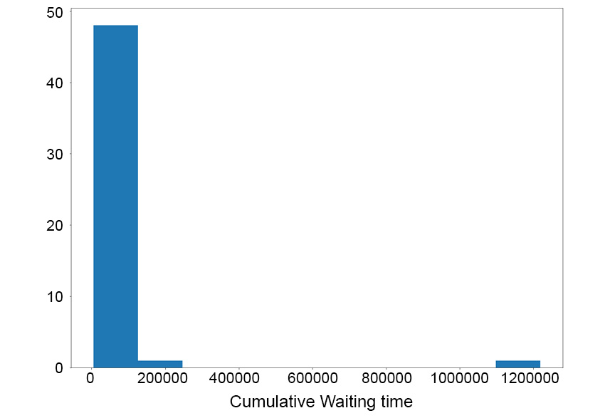
Figure 8.23: Distribution of cumulative waiting time from modified Thompson Sampling
The max and mean cumulative waiting times will be as follows:
(1218887.7924350922, 45093.244027644556)
Note
The solution to this activity can be found on page 734.
Summary
In this chapter, the MAB problem and its motivation as a reinforcement learning and artificial intelligence problem were introduced. We explored a plethora of algorithms that are commonly used to solve the MAB problem, including the Greedy algorithm and its variants, UCB, and Thompson Sampling. Via these algorithms, we were exposed to unique insights and heuristics on how to balance exploration and exploitation (which is one of the most fundamental components of reinforcement learning) such as random exploration, optimism under uncertainty, or sampling from Bayesian posterior distributions.
This knowledge was put into practice as we learned how to implement these algorithms from scratch in Python. During this process, we also examined the importance of analyzing MAB algorithms over many repeated experiments to obtain robust results. This procedure is integral for any analysis framework that involves randomness. Finally, in this chapter's activity, we applied our knowledge to a queueing bandit problem and learned how to modify MAB algorithms so that they fit a given contextual bandit.
This chapter also marks the end of the topic of Markov decision problems, which spanned the last four chapters. From the next chapter onward, we will start looking at the exciting field of Deep Q Learning as a reinforcement learning framework.