
Overview
This chapter introduces you to some key technologies and concepts to get started with reinforcement learning. You will become familiar with and use two OpenAI tools: Gym and Universe. You will learn how to deal with the interfaces of these environments and how to create a custom environment for a specific problem. You will build a policy network with TensorFlow, feed it with environment states to retrieve corresponding actions, and save the policy network weights. You will also learn how to use another OpenAI resource, Baselines, and use it to train a reinforcement learning agent to solve a classic control problem. By the end of this chapter, you will be able to use all the elements we will introduce to build and train an agent to play a classic Atari video game, thus achieving better-than-human performance.
Introduction
In the previous chapter, you were introduced to TensorFlow and Keras, along with an overview of their key features and applications and how they work in synergy. You learned how to implement a deep neural network with TensorFlow, addressing all major topics, that is, model creation, training, validation, and testing, using the most advanced machine learning frameworks available. In this chapter, we will use this knowledge to build models that are able to solve some classical reinforcement learning problems.
Reinforcement learning is a branch of machine learning that comes closest to the idea of artificial intelligence. The goal of training an artificial system to learn a given task, without any prior information, and only by means of experiences of an environment, represents the ambitious aim of replicating human learning. Applying deep learning techniques to the field has recently led to a great increase in performance, thus allowing us to solve problems in very different domains, from classic control problems to video games and even robotic locomotion. This chapter will introduce the various resources, methods, and tools you can use to become familiar with the context and problems typically encountered when getting started in the field. In particular, we will look at OpenAI Gym and OpenAI Universe, two libraries that allow us to easily create environments where we can train Reinforcement Learning (RL) agents, and OpenAI Baselines, a tool that provides a clear and simple interface for state-of-the-art reinforcement learning algorithms. By the end of this chapter, you will be able to leverage top libraries and modules to easily train a state-of-the-art reinforcement learning agent to solve classic control problems, as well as to achieve better-than-human performance on classic video games.
Now, let's begin our journey, starting with the very first important concept: how to correctly model a proper reinforcement learning environment where we can train an agent. For this, we will be using OpenAI Gym and Universe.
OpenAI Gym
In this section, we will study the OpenAI Gym tool. We will go through the motivations behind its creation and its main elements, learning how to interact with them to properly train a reinforcement learning algorithm to tackle state-of-the-art benchmark problems. Finally, we will build a custom environment with the same set of standardized interfaces.
The role of shared standard benchmarks for machine learning algorithms is of paramount importance to measure performance and state-of-the-art improvements. While for supervised learning there have been many different examples since the early days of the discipline, the same is not true for the reinforcement learning field.
With the aim of fulfilling this need, in 2016, OpenAI released OpenAI Gym (https://gym.openai.com/). It was conceived to be to reinforcement learning what standardized datasets such as ImageNet and COCO are to supervised learning: a standard, shared context in which the performance of RL methods can be directly measured and compared, both to identify the highest-achieving ones as well as to monitor current progress.
OpenAI Gym acts as an interface between the typical Markov decision process formulation of the reinforcement learning problem and a variety of environments, covering different types of problems the agent has to solve (from classic control to Atari video games), as well as different observations and action spaces. Gym is completely independent of the structure of the agent that will be interfaced with, as well as the machine learning framework used to build and run it.
Here is the list of environment categories Gym offers, ranging from easy to difficult and involving many different kinds of data:
- Classic control and toy text: Small-scale easy tasks, frequently found in reinforcement learning literature. These environments are the best place to start in order to gain confidence with Gym and to familiarize yourself with agent training.
The following figure shows an example of classic control problem of CartPole:
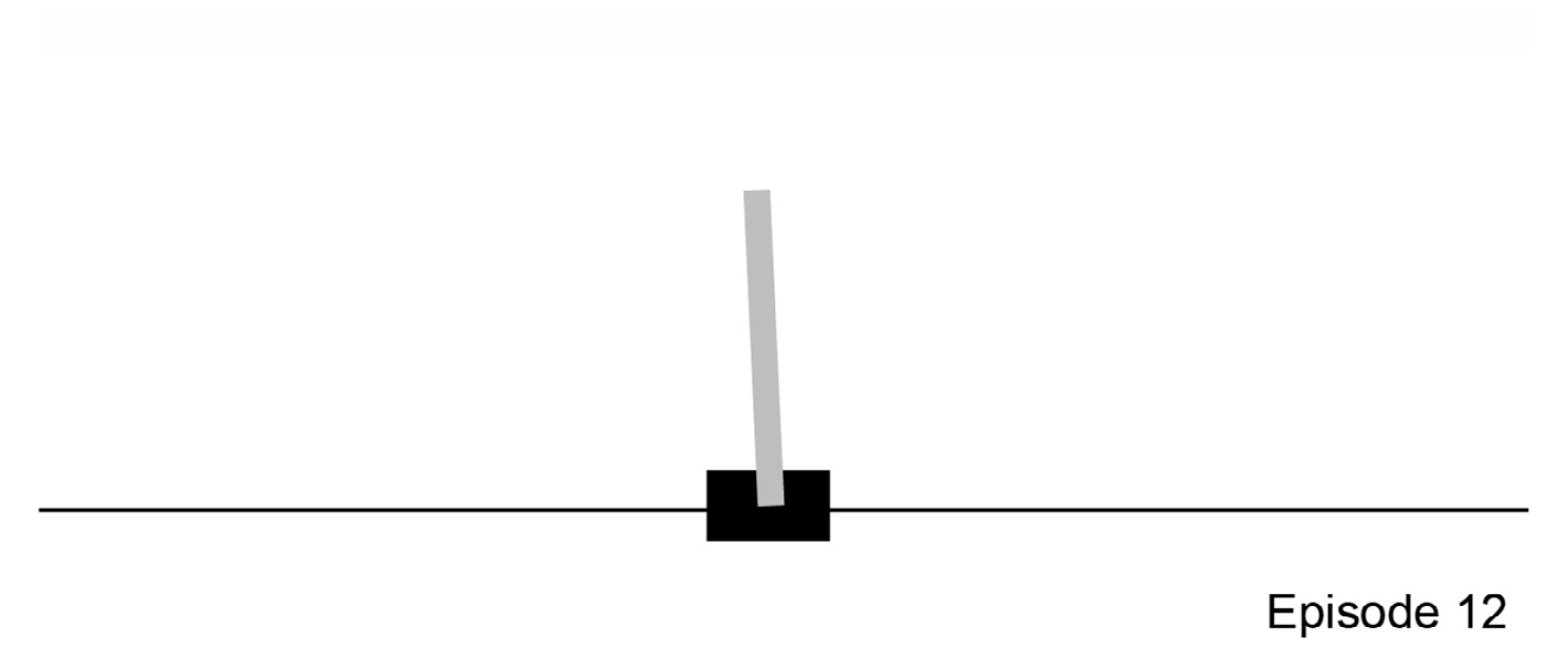
Figure 4.1: Classic control problem- CartPole
The following figure shows an example of classic control problem of MountainCar:
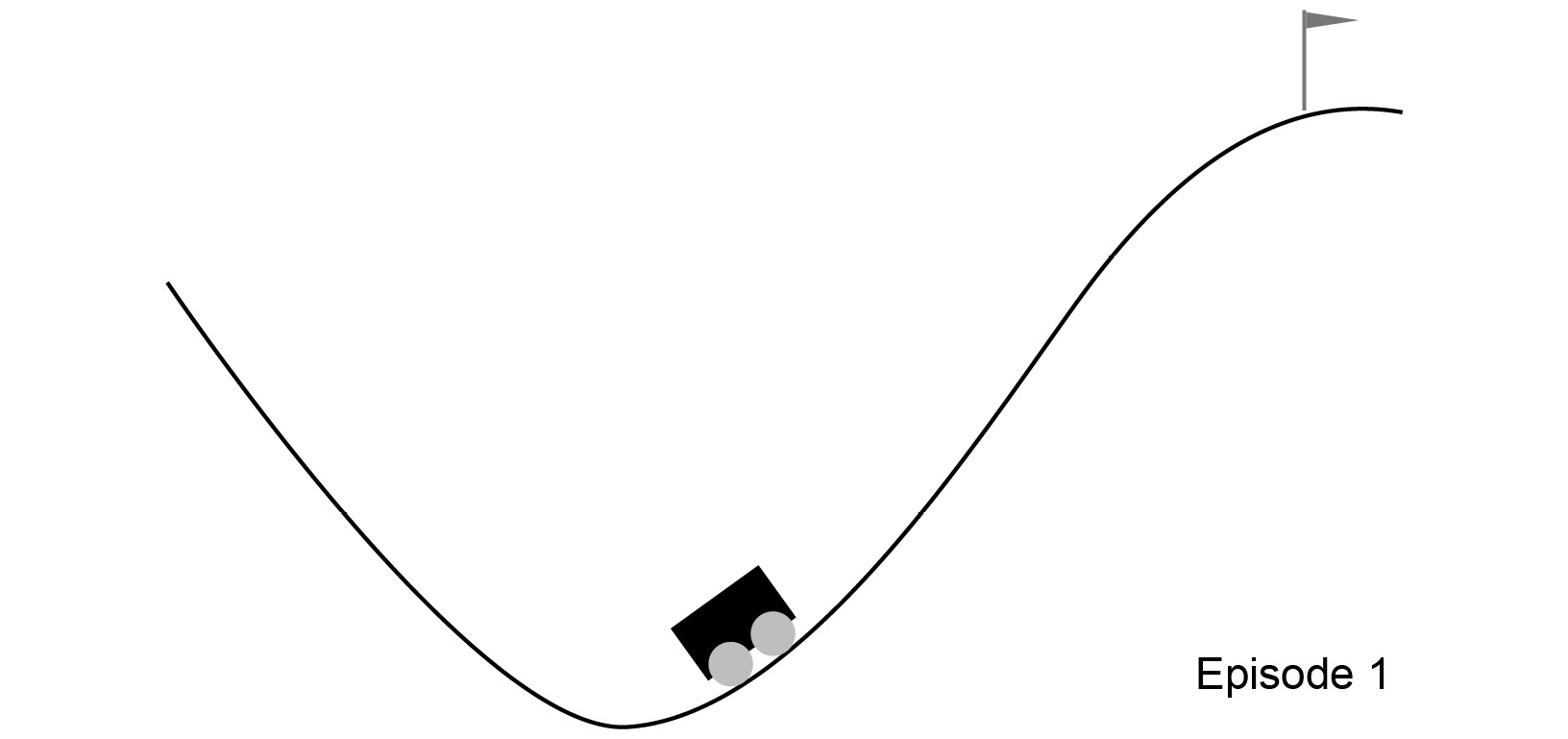
Figure 4.2: Classic control problem - Mountain Car
- Algorithmic: In these environments, the system has to learn, autonomously and purely from examples, to perform computations ranging from multi-digit additions to alphanumeric-character sequence reversal.
The following figure shows screenshot representing instances of the algorithmic problem set:
Figure 4.3: Algorithmic problem – copying multiple instances of the input sequence
The following figure shows screenshot representing instances of the algorithmic problem set:
Figure 4.4: Algorithmic problem - copying instance of the input sequence
- Atari: Gym integrates the Arcade Learning Environment (ALE), a software library that provides an interface we can use to train an agent to play classic Atari video games. It played a major role in helping reinforcement learning research achieve outstanding results.
The following figure shows Atari video game Breakout, provided by ALE:
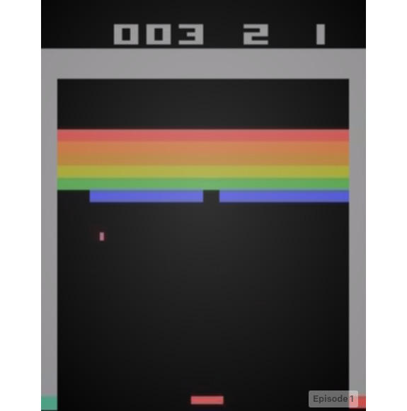
Figure 4.5: Atari video game of Breakout
The following figure shows Atari video game Pong, provided by ALE:
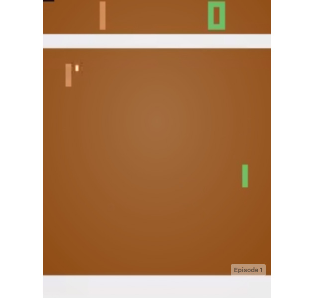
Figure 4.6: Atari video game of Pong
Note
The preceding figures have been sourced from the official documentation for OpenAI Gym. Please refer to the following link for more visual examples of Atari games: https://gym.openai.com/envs/#atari.
- MuJoCo and Robotics: These environments expose typical challenges that are encountered in the field of robot control. Some of them take advantage of the MuJoCo physics engine, which was designed for fast and accurate robot simulation and offers free licenses for trial.
The following figure shows three MuJoCo environments, all of which provide a meaningful overview of robotic locomotion tasks:
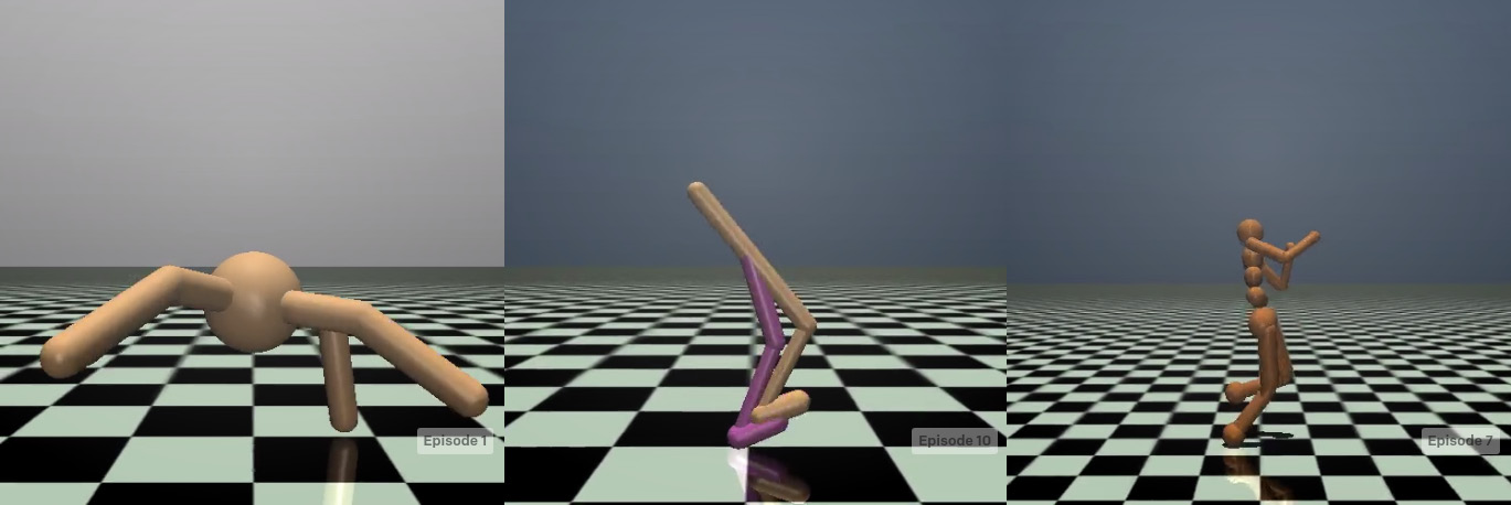
Figure 4.7: Three MuJoCo-powered environments – Ant (left), Walker (center), and Humanoid (right)
Note
The preceding images have been sourced from the official documentation for OpenAI Gym. Please refer to the following link for more visual examples of MuJoCo environments: https://gym.openai.com/envs/#mujoco.
- The following figure shows two environments contained in the "Robotics" category, where RL agents are trained to perform robotic manipulation tasks:
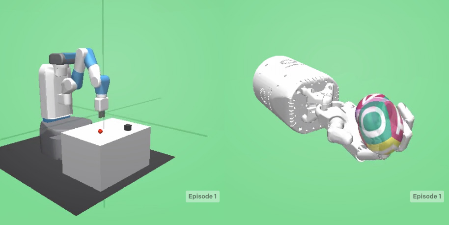
Figure 4.8: Two robotics environments – FetchPickAndPlace (left) and HandManipulateEgg (Right)
Note
The preceding images have been sourced from the official documentation for OpenAI Gym. Please refer to the following link for more visual examples of Robotics environments: https://gym.openai.com/envs/#robotics.
- Third-party environments: Environments developed by third parties are also available with a very broad landscape of applications, complexity, and data types (https://github.com/openai/gym/blob/master/docs/environments.md#third-party-environments).
How to Interact with a Gym Environment
In order to interact with a Gym environment, it has to, first of all, be created and initialized. The Gym module uses the make method, along with the ID of the environment as an argument, to create and return a new instance of it. To list all available environments in a given Gym installation, it is sufficient to just run the following code:
from gym import envs
print(envs.registry.all())
This prints out the following:
[EnvSpec(DoubleDunk-v0), EnvSpec(InvertedDoublePendulum-v0),
EnvSpec(BeamRider-v0), EnvSpec(Phoenix-ram-v0), EnvSpec(Asterix-v0),
EnvSpec(TimePilot-v0), EnvSpec(Alien-v0), EnvSpec(Robotank-ram-v0),
EnvSpec(CartPole-v0), EnvSpec(Berzerk-v0), EnvSpec(Berzerk-ram-v0),
EnvSpec(Gopher-ram-v0), ...
This is a list of so-called EnvSpec objects. They define specific environment-related parameters, such as the goal to be achieved, the reward threshold defining when the task is considered solved, and the maximum number of steps allowed for a single episode.
One interesting thing to note is that it is possible to easily add custom environments, as we will see later on. Thanks to this, a user can implement a custom problem using standard interfaces, making it straightforward for it to be tackled by standardized, off-the-shelf, reinforcement learning algorithms.
The fundamental elements of an environment are as follows:
- Observation (object): An environment-specific object representing what can be observed of the environment; for example, the kinematic variables (that is, velocities and positions) of a mechanical system, pawn positions in a chess game, or the pixel frames of a video game.
- Actions (object): An environment-specific object representing actions the agent can perform in the environment; for example, joint rotations and/or joint torques for a robot, a legal move in a board game, or buttons being pressed in combination for a video game.
- Reward (float): The amount of reward achieved by executing the last step with the prescribed action. The reward range differs between different tasks, but in order to solve the environment, the aim is always to increase it, since this is what the RL agent tries to maximize.
- Done (bool): This indicates whether the episode has finished. If true, the environment needs to be reset. Most, but not all, tasks are divided into well-defined episodes, where a terminated episode may represent that the robot has fallen on the ground, the board game has reached a final state, or the agent lost its last life in a video game.
- Info (dict): This contains diagnostic information on environment internals and is useful for both debugging purposes and for an RL agent training, even if it's not allowed for standard benchmark comparisons.
The fundamental methods of an environment are as follows:
- reset(): Input: none, output: observation. Resets the environment, bringing it to the starting point. It takes no input and outputs the corresponding observation. It has to be called right after environment creation and every time a final state is reached (done flag equal to True).
- step(action): Input: action, output: observation – reward – done – info. Advances the environment by one step, applying the selected input action. Returns the observation of the newly reached state, which is a reward associated with the transition from the previous to the new state under the selected action. The done flag is used to indicate whether the new state is a terminal one or not (True/False, respectively), as well as the Info dict with environment internals.
- render(): Input: none, output: environment rendering. Renders the environment and is used for visualization/presentation purposes only. It is not used during agent training, which only needs observations to know the environment's state. For example, it presents robot movements via animation graphics or outputs a video game video stream.
- close(): Input: none, output: none. Shuts down the environment gracefully.
These elements allow us to have complete interaction with the environment simply by executing it with random inputs, training an agent, and running it. It is, in fact, an implementation of the standard reinforcement learning contextualization, which is described by the agent-environment interaction. For each timestep, the agent executes an action. This interaction with the environment causes a transition from the current state to a new state, resulting in an observation of the new state and a reward, which are returned as results. As a preliminary step, the following exercise shows how to create a CartPole environment, reset it, run it for 1,000 steps while randomly sampling one action for each step, and finally close it.
Exercise 4.01: Interacting with the Gym Environment
In this exercise, we will familiarize ourselves with the Gym environment by looking at a classic control example, CartPole. Follow these steps to complete this exercise:
- Import the OpenAI Gym module:
import gym
- Instantiate the environment and reset it:
env = gym.make('CartPole-v0')
env.reset()
The output will be as follows:
array([ 0.03972635, 0.00449595, 0.04198141, -0.01267544])
- Run the environment for 1000 steps, rendering it and resetting it if a terminal state is encountered. After all steps are completed, close the environment:
for _ in range(1000):
env.render()
# take a random action
_, _, done, _ = env.step(env.action_space.sample())
if done:
env.reset()
env.close()
It renders the environment and plays it for 1,000 steps. The following figure shows one frame that was extracted from step number 12 of the entire sequence:
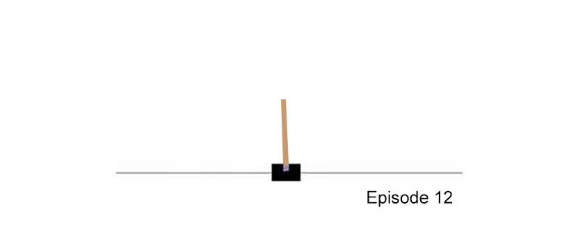
Figure 4.9: One frame of the 1,000 rendered steps for the CartPole environment
Note
To access the source code for this specific section, please refer to https://packt.live/30yFmOi.
This section does not currently have an online interactive example, and will need to be run locally.
This shows that the black cart can move along its rail (the horizontal line), with its pole fixed on the cart with a hinge that allows it to rotate freely. The goal is to control the cart while pushing it left and right in order to maintain the pole's vertical equilibrium, as seen in the preceding figure.
Action and Observation Spaces
In order to appropriately interact with an environment and train an agent on it, a fundamental initial step is to familiarize yourself with its action and observation spaces. For example, in the preceding exercise, the action was randomly sampled from the environment's action space.
Every environment is characterized by action_space and observation_space, which are instances of the Space class that describe the actions and observations required by Gym. The following snippet prints them out for the CartPole environment:
import gym
env = gym.make('CartPole-v0')
print("Action space =", env.action_space)
print("Observation space =", env.observation_space)
This outputs the following two rows:
Action space = Discrete(2)
Observation space = Box(4,)
The Discrete space represents the set of non-negative integer numbers (natural numbers plus 0). Its dimension defines which numbers represent valid actions. For example, in the CartPole case, it is of dimension 2 because the agent can only push the cart left and right, so the admissible values are 0 or 1. The Box space can be thought of as an n-dimensional array. In the CartPole case, the system state is defined by four variables: cart position and velocity, and pole angle with respect to the vertical and angular velocity. So, the "box observation" space dimension is equal to 4, and valid observations will be an array of four real numbers. In the latter case, it is useful to check their upper and lower bounds. This can be done as follows:
print("Observations superior limit =", env.observation_space.high)
print("Observations inferior limit =", env.observation_space.low)
This prints out the following:
Observations superior limit = array([ 2.4, inf, 0.20943951, inf])
Observations inferior limit = array([-2.4, -inf,-0.20943951, -inf])
With these new elements, it is possible to write a more complete snippet to interact with the environment, using all the previously presented interfaces. The following code shows a complete loop, executing 20 episodes, each for 100 steps, rendering the environment, retrieving observations, and printing them out while taking random actions and resetting once it reaches a terminal state:
import gym
env = gym.make('CartPole-v0')
for i_episode in range(20):
observation = env.reset()
for t in range(100):
env.render()
print(observation)
action = env.action_space.sample()
observation, reward, done, info = env.step(action)
if done:
print("Episode finished after {} timesteps".format(t+1))
break
env.close()
The preceding code runs the environment for 20 episodes of 100 steps each, also rendering the environment, as we saw in Exercise 4.01, Interacting with the Gym Environment.
Note
In the preceding case, we run each episode for 100 steps instead of 1,000, as we did previously. There is no particular reason for doing so, but we are running 20 different episodes, not a single one, so we opted for 100 steps to keep the code execution time short enough.
In addition to that, this code also prints out the sequence of observations, as returned by the environment, for each step performed. The following are a few lines that are received as output:
[-0.061586 -0.75893141 0.05793238 1.15547541]
[-0.07676463 -0.95475889 0.08104189 1.46574644]
[-0.0958598 -1.15077434 0.11035682 1.78260485]
[-0.11887529 -0.95705275 0.14600892 1.5261692 ]
[-0.13801635 -0.7639636 0.1765323 1.28239155]
[-0.15329562 -0.57147373 0.20218013 1.04977545]
Episode finished after 14 timesteps
[-0.02786724 0.00361763 -0.03938967 -0.01611184]
[-0.02779488 -0.19091794 -0.03971191 0.26388759]
[-0.03161324 0.00474768 -0.03443415 -0.04105167]
Looking at the previous code example, we can see how, for now, the action choice is completely random. It is right here that a trained agent would make a difference: it should choose actions based on environment observations, thus appropriately responding to the state it finds itself in. So, revising the previous code by substituting a trained agent in place of a random action choice looks as follows:
- Import the OpenAI Gym and CartPole modules:
import gym
env = gym.make('CartPole-v0')
- Run 20 episodes of 100 steps each:
for i_episode in range(20):
observation = env.reset()
for t in range(100):
- Render the environment and print the observation:
env.render()
print(observation)
- Use the agent's knowledge to choose the action, given the current environment state:
action = RL_agent.select_action(observation)
- Step the environment:
observation, reward, done, info = env.step(action)
- If successful, break the inner loop and start a new episode:
if done:
print("Episode finished after {} timesteps"
.format(t+1))
break
env.close()
With a trained agent, actions will be chosen optimally since a function of the state that the agent is in, is used to maximize the expected reward. This code would result in an output similar to the previous one.
But how do we proceed and train an agent from scratch? As you will learn throughout this book, there are many different approaches and algorithms we can use to achieve this quite complex task. In general, they all need the following tuple of elements: current state, chosen action, reward obtained by performing the chosen action, and new state reached by performing the chosen action.
So, elaborating again on the previous code snippet to introduce the agent training step, it would look like this:
import gym
env = gym.make('CartPole-v0')
for i_episode in range(20):
observation = env.reset()
for t in range(100):
env.render()
print(observation)
action = RL_agent.select_action(observation)
new_observation, reward, done, info = env.step(action)
RL_agent.train(observation, action, reward,
new_observation)
observation = new_observation
if done:
print("Episode finished after {} timesteps"
.format(t+1))
break
env.close()
The only difference in this code with respect to the previous block is the following line:
RL_agent.train(observation, action, reward, new_observation)
This refers to the agent training step. The purpose of this code is to give us a high-level idea of all the steps involved in training an RL agent in a given environment.
This is the high-level idea behind the method adopted to carry out reinforcement learning agent training with the Gym environment. It provides access to all the required details through a very clean standard interface, thus giving us access to an extremely large set of different problems against which measuring algorithms and techniques can be used.
How to Implement a Custom Gym Environment
All the environments that are available through Gym are perfect for learning purposes, but eventually, you will need to train an agent to solve a custom problem. One good way to achieve this is to create a custom environment, specific to the problem domain.
In order to do so, a class derived from gym.Env must be created. It will implement all the objects and methods described in the previous section so that it supports the agent-world interaction cycle that's typical of any reinforcement learning setting.
The following snippet represents a frame guiding a custom environment's development:
import gym
from gym import spaces
class CustomEnv(gym.Env):
"""Custom Environment that follows gym interface"""
metadata = {'render.modes': ['human']}
def __init__(self, arg1, arg2, ...):
super(CustomEnv, self).__init__()
# Define action and observation space
# They must be gym.spaces objects
# Example when using discrete actions:
self.action_space = spaces.Discrete(N_DISCRETE_ACTIONS)
# Example for using image as input:
self.observation_space = spaces.Box
(low=0, high=255,
shape=(HEIGHT, WIDTH,
N_CHANNELS),
dtype=np.uint8)
def step(self, action):
# Execute one time step within the environment
...
# Compute reward
...
# Check if in final state
...
return observation, reward, done, info
def reset(self):
# Reset the state of the environment to an initial state
...
return observation
def render(self, mode='human', close=False):
# Render the environment to the screen
...
return
In the constructor, action_space and observation_space are defined. As mentioned previously, they will contain all possible actions the agent can take in the environment and all environment data observable by the agent. They are to be attributed to the specific problem: in particular, action_space will reflect elements the agent can control to interact with the environment, while observation_space will contain all the variables we want the agent to consider when choosing the action.
The reset method will be called to periodically reset the environment to an initial state, typically after the first initialization and every time after the end of an episode. It will return the observation.
The step method receives an action as input and executes it. This will result in an environment transitioning from the current state to a new state. The observation related to the new state is returned. This is also the method where the reward is calculated as a result of the state transition generated by the action. The new state is checked to determine whether it is a terminal one, in which case, the done flag that's returned is set to true. As the last step, all useful internals are returned in the info dictionary.
Finally, the render method is the one in charge of rendering the environment. Its complexity may range from being as simple as a print statement to being as complicated as rendering a 3D environment using OpenGL.
In this section, we studied the OpenAI Gym tool. We had an overview that explained the context and motivations behind its conception, provided details about its main elements, and saw how to interact with the elements to properly train a reinforcement learning algorithm to tackle state-of-the-art benchmark problems. Finally, we saw how to build a custom environment with the same set of standardized interfaces.
OpenAI Universe – Complex Environment
OpenAI Universe was released by OpenAI a few months after Gym. It's a software platform for measuring and training artificial general intelligence on different applications, ranging from video games to websites. It makes an AI agent able to use a computer as a human does: the environment state is represented by screen pixels and the actions are all operations that can be performed by operating a virtual keyboard and mouse.
With Universe, it is possible to adapt any program, thus transforming the program into a Gym environment. It executes the program using Virtual Network Computing (VNC) technology, a software technology that allows the remote control of a computer system via graphical desktop-sharing over a network, transmitting keyboard and mouse events and receiving screen frames. By mimicking execution behind a remote desktop, it doesn't need to access program memory states, customized source code, or have a set of APIs.
The following snippet shows how to use Universe in a simple Python program, where a scripted action is always executed in every step:
- Import the OpenAI Gym and OpenAI Universe modules:
import gym
# register Universe environments into Gym
import universe
- Instantiate the OpenAI Universe environment and reset it:
# Universe env ID here
env = gym.make('flashgames.DuskDrive-v0')
observation_n = env.reset()
- Execute a prescribed action to interact with the environment and render it:
while True:
# agent which presses the Up arrow 60 times per second
action_n = [[('KeyEvent', 'ArrowUp', True)]
for _ in observation_n]
observation_n, reward_n, done_n, info = env.step(action_n)
env.render()
The preceding code successfully runs a Flash game in the browser.
The goal behind Universe is to favor the development of an AI agent that's capable of applying its past experience to master complex new environments, which would represent a fundamental step in the quest for artificial general intelligence.
Despite the great success of AI in recent years, all developed systems can still be considered "Narrow AI." This is because they can only achieve better-than-human performance in a limited domain. Building something with a general problem-solving ability on a par with human common sense requires overcoming the goal of carrying agent experience along when shifting to a completely new task. This would allow an agent to avoid training from scratch, randomly going through tens of millions of trials.
Now, let's take a look at the infrastructure of OpenAI Universe.
OpenAI Universe Infrastructure
The following diagram effectively describes how OpenAI Universe works: it exposes all its environments, which will be described in detail later, through a common interface: by leveraging VNC technology, it makes the environment act as a server and the agent as a client so that the latter operates a remote desktop by observing the pixels of a screen (observations of the environment) and producing keyboard and mouse commands (actions of the agent). VNC is a well-established technology and is the standard for interacting with computers remotely through the network, as in the case of cloud computing systems or decentralized infrastructures:
Figure 4.10: VNC server-client Universe infrastructure
Universe's implementation has some notable properties, as follows:
- Generality: By adopting the VNC interface, it doesn't require emulators or access to a program's source code or memory states, thus opening a relevant number of opportunities in fields such as computer games, web browsing, CAD software usage, and much more.
- Familiarity to humans: It can be easily used by humans to provide baselines for AI algorithms, which are useful to initialize agents with human demonstrations recorded in the form of VNC traffic. For example, a human can solve one of the tasks provided by OpenAI Universe by using it through VNC and recording the corresponding traffic. Then, it can use it to train an agent, providing good examples of policies to learn from.
- Standardization. Leveraging VNC technology ensures portability in all major operating systems that have VNC software by default.
- Easiness of debugging: It is super easy to observe the agent during training or evaluation by simply connecting a client for visualization to the environment's VNC shared server. Saving VNC traffic also helps.
Environments
In this section, we will look at the most important categories of problems that are already available inside Universe. Each environment is composed of a Docker image and hosts a VNC server. The server has the role of the interface and is in charge of the following:
- Sending observations (screen pixels)
- Receiving actions (keyboard/mouse commands)
- Providing information for reinforcement learning tasks (reward signal, diagnosis elements, and so on) through a Web Socket server
Now, let's take a look at each of the different categories of environments.
Atari Games
These are the classic Atari 2600 games from the ALE. Already encountered in OpenAI Gym, they are also part of Universe.
Flash Games
The landscape of Flash games offers a large number of games with more advanced graphics with respect to Atari, but still with simple mechanics and goals. Universe's initial release contained 1,000 Flash games, 100 of which also provided reward as a function.
With the Universe approach, there is a major aspect to be addressed: how the agent knows how well it performed, which is related to the rewards returned by interacting with the environment. If you don't have access to an application's internal states (that is, its RAM addresses), the only way to do so is to extract such information from the onscreen pixels. Many games have a score associated with them, and this is printed out on each frame so that it can be parsed via some image processing algorithm. For example, Atari Pong shows both players' scores in the top part of the frame, so it is possible to parse those pixels to retrieve it. Universe developed a high-performing image-to-text model based on convolutional neural networks that's embedded into the Python controller and runs inside a Docker container. On the environments where it can be applied, it retrieves the user's score from the frame buffer and provides this information through the Web Socket's score from the frame buffer, thus providing this information through the Web Socket.
Browser Tasks
Universe adds a unique set of tasks based on the usage of a web browser. These environments put the AI agent in front of a common web browser, presenting it with problems that require the use of the web: reading content, navigating through pages and clicking buttons while observing only pixels, and using the keyboard and mouse. Depending on the complexity, these tasks can, conceptually, be grouped into two categories: Mini World of Bits and real-world browser tasks:
- Mini World of Bits:
These environments are to browser-based tasks as what the MNIST dataset is to image recognition: they are basic building blocks that can be found on complex browsing problems on which training is easier but also insightful. They are environments of differing difficulty levels, for example, that you click on a specific button or reply to a message using an email client.
- Real-world browser tasks:
With respect to the previous category, these environments require the agent to solve more realistic problems, usually in the form of an instruction expressed to the agent, which has to perform a sequence of actions on a website. An example could be a request for an agent to book a specific flight that would require it to interact with the platform in order to find the right answer.
Running an OpenAI Universe Environment
Being a large collection of tasks that can be accessed via a common interface, running an environment requires performing only a few steps:
- Install Docker and Universe, which can be done with the following command:
git clone https://github.com/openai/universe && pip install -e universe
- Start a runtime, which is a server that groups a collection of similar environments into a "runtime" exposing two ports: 5900 and 15900. Port 5900 is used for the VNC protocol to exchange pixel information or keyboard/mouse actions, while 15900 is used to maintain the WebSocket control protocol. The following snippet shows how to boot a runtime from a PC console (for example, a Linux shell):
# -p 5900:5900 and -p 15900:15900
# expose the VNC and WebSocket ports
# --privileged/--cap-add/--ipc=host
# needed to make Selenium work
$ docker run --privileged --cap-add=SYS_ADMIN --ipc=host
-p 5900:5900 -p 15900:15900 quay.io/openai/universe.flashgames
With this command, the Flash game's Docker container will be downloaded. You can then use a VNC viewer to view and control the created remote desktop. The target port is 5900. It is also possible to use the browser-based VNC client through the web server using port 15900 and the password openai.
The following snippet is the very same as the one we saw previously, except it only adds the VNC connection step. This means that the output is also the same, so it is not reported here. As we saw, writing a custom agent is quite straightforward. Observations include a NumPy pixel array, and actions are a list of VNC events (mouse/keyboard interactions):
import gym
import universe # register Universe environments into Gym
# Universe [environment ID]
env = gym.make('flashgames.DuskDrive-v0')
"""
If using docker-machine, replace "localhost" with specific Docker IP
"""
env.configure(remotes="vnc://localhost:5900+15900")
observation_n = env.reset()
while True:
# agent which presses the Up arrow 60 times per second
action_n = [[('KeyEvent', 'ArrowUp', True)]
for _ in observation_n]
observation_n, reward_n, done_n, info = env.step(action_n)
env.render()
Exploiting the same VNC connection, the user is able to watch the agent in action and also send action commands using the keyboard and mouse. The VNC interface, managing environments as server processes, allows us to run them on remote machines, thus allowing us to leverage in-house computation clusters or even cloud solutions. For more information, refer to the OpenAI Universe website (https://openai.com/blog/universe/).
Validating the Universe Infrastructure
One of the intrinsic problems of Universe is the associated lag in observations and execution of actions that comes with the choice of architecture. In fact, agents must operate in real time and are accountable for fluctuating action and observation delays. Most environments can't be solved with current techniques, but the creators of Universe performed tests to guarantee that it is actually possible for an RL agent to learn. During these tests, the reward trends during training for Atari games, Flash games, and browser tasks confirm that it is actually possible to obtain results even in such a complex setting.
Now that we've introduced the OpenAI tools for reinforcement learning, we can now move on and learn how to use TensorFlow in this context.
TensorFlow for Reinforcement Learning
In this section, we will learn how to create, run, and save a policy network using TensorFlow. Policy networks are one of the fundamental pieces, if not the most important one, of reinforcement learning. As will be shown throughout this book, they are a very powerful implementation of containers for the knowledge the agent has to learn, which tells them how to choose actions based on environment observations.
Implementing a Policy Network Using TensorFlow
Building a policy network is not too different from building a common deep learning model. Its goal is to output the "optimal" action, given the input it receives, that represents the environment's observation. So, it acts as a link between the environment state and the optimal agent behavior associated with it. Being optimal here means doing what maximizes the cumulative expected reward of the agent.
To make things as clear as possible, we will focus on a specific problem here, but the same approach can be adopted to solve other tasks, such as controlling a robotic arm or teaching locomotion to a humanoid robot. We will see how to create a policy network for a classic control problem that will also be at the core of an exercise later in this chapter. This problem is the "CartPole" problem: the goal is to maintain the balance of the vertical pole so that it is upright at all times. Here, the only way to do this is by moving the cart along either direction of the x-axis. The following figure shows a frame from this problem:
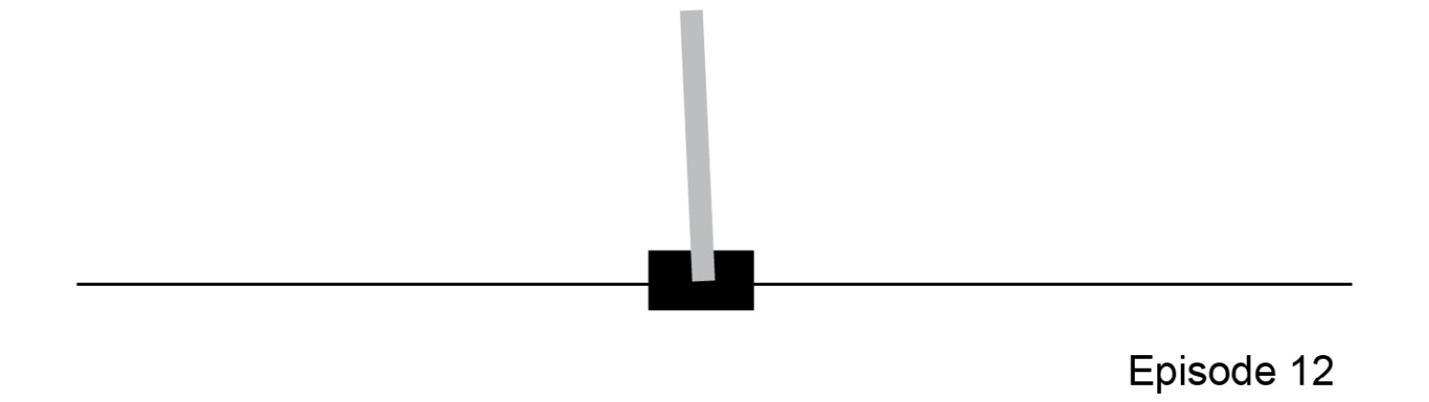
Figure 4.11: CartPole control problem
As we mentioned previously, the policy network links the observations of the environment with the actions that the agent can take. So, they act as the input and output, respectively.
As we saw in the previous chapter, this is the first information that you need in order to build a neural network. To retrieve the input and output dimensions, you have to instantiate the environment (in this case, this is done via OpenAI Gym) and print out information about the observation and action spaces.
Let's perform this first task by completing the following exercise.
Exercise 4.02: Building a Policy Network with TensorFlow
In this exercise, we will learn how to build a policy network with TensorFlow for a given Gym environment. We will learn how to take its observation space and action space into account, which constitute the input and output of the network, respectively. We will then create a deep learning model that is able to generate actions for the agent in the environment in response to environment observations. This network is the piece that needs to be trained and is the final goal of every RL algorithm. Follow these steps to complete this exercise:
- Import the required modules:
import numpy as np
import gym
import tensorflow as tf
- Instantiate the environment:
env = gym.make('CartPole-v0')
- Print out the action and observation spaces:
print("Action space =", env.action_space)
print("Observation space =", env.observation_space)
This prints out the following:
Action space = Discrete(2)
Observation space = Box(4,)
- Print out the action and observation space dimensions:
print("Action space dimension =", env.action_space.n)
print("Observation space dimension =",
env.observation_space.shape[0])
The output will be as follows:
Action space dimension = 2
Observation space dimension = 4
As you can see from the preceding output, the action space is a discrete space of dimension 2, meaning it can take the value 0 or 1. The observation space is of the Box type with a dimension of 4, meaning it consists of four real numbers inside the lower and upper boundaries, which, as we already saw for the CartPole environment, are [±2.4, ± inf, ±0.20943951, ±inf].
With this information, it is now possible to build a policy network that can be interfaced with the CartPole environment. The following code block shows one of many possible choices: it uses two hidden layers with 64 neurons each and an output layer with 2 neurons (as this is the action space's dimension) with a softmax activation function. The model summary prints out the outline of the model.
- Build the policy network and print its summary:
model = tf.keras.Sequential
([tf.keras.layers.Dense(64, activation='relu',
input_shape=[env.observation_space.shape[0]]),
tf.keras.layers.Dense(64, activation='relu'),
tf.keras.layers.Dense(env.action_space.n,
activation="softmax")])
model.summary()
The output will be as follows:
Model: "sequential_2"
_________________________________________________________________
Layer (type) Output Shape Param # =================================================================
dense (Dense) (None, 64) 320 _________________________________________________________________
dense_1 (Dense) (None, 64) 4160 _________________________________________________________________
dense_2 (Dense) (None, 2) 130 =================================================================
Total params: 4,610
Trainable params: 4,610
Non-trainable params: 0
As you can see, the model has been created and we also have an elaborate summary of it, which gives us significant information about the model, regarding the layers, the parameters of the network, and so on.
Note
To access the source code for this specific section, please refer to https://packt.live/3fkxfce.
You can also run this example online at https://packt.live/2XSXHnF.
Once the policy network has been built and initialized, it is possible to feed it. Of course, since the network hasn't been trained, it will generate random outputs, but still, it can be used, for example, to run a random agent in an environment of choice. This is what we will implement in the following exercise: the neural network model will be fed with the observation provided by the environment step or reset function through the predict method. This outputs the action probabilities. The action with the highest probability is chosen and used to step through the environment until the episode ends.
Exercise 4.03: Feeding the Policy Network with Environment State Representation
In this exercise, we will be feeding information to the policy network with the environment state representation. This exercise is a continuation of Exercise 4.02, Building a Policy Network with TensorFlow, so in order to carry it out, you need to perform all the steps of the preceding exercise and then begin this one right after. Follow these steps to complete this exercise:
- Reset the environment:
t = 1
observation = env.reset()
- Start a loop that will run until the episode is complete. Render the environment and print the observations:
while True:
env.render()
# Print the observation
print("Observation = ", observation)
- Feed the network with the environment observations, let it choose the appropriate actions, and print it:
action_probabilities =model.predict
(np.expand_dims(observation, axis=0))
action = np.argmax(action_probabilities)
print("Action = ", action)
- Step through the environment with the selected action. Print the received reward and close the environment if the terminal state has been reached:
observation, reward, done, info = env.step(action)
# Print received reward
print("Reward = ", reward)
# If terminal state reached, close the environment
if done:
print("Episode finished after {} timesteps".format(t+1))
break
t += 1
env.close()
This produces the following output (only the last few lines have been shown):
Observation = [-0.00324467 -1.02182257 0.01504633 1.38740738]
Action = 0
Reward = 1.0
Observation = [-0.02368112 -1.21712879 0.04279448 1.684757 ]
Action = 0
Reward = 1.0
Observation = [-0.0480237 -1.41271906 0.07648962 1.99045154]
Action = 0
Reward = 1.0
Observation = [-0.07627808 -1.60855467 0.11629865 2.30581208]
Action = 0
Reward = 1.0
Observation = [-0.10844917 -1.80453455 0.16241489 2.63191088]
Action = 0
Reward = 1.0
Episode finished after 11 timesteps
Note
To access the source code for this specific section, please refer to https://packt.live/2AmwUHw.
You can also run this example online at https://packt.live/3kvuhVQ.
By completing this exercise, we've built a policy network and used it to guide an agent's behavior in a Gym environment. At the moment, it behaves randomly, but apart from policy network training, which will be explained in the following chapters, every other piece of the big picture is already in place.
How to Save a Policy Network
The goal of reinforcement learning is to effectively train the network so that it learns how to perform the optimal action for every given environment state. RL theory deals with how to achieve this goal and, as we will see, different approaches have been successful. Supposing one of them has been applied to the previous network, the trained model needs to be saved so that it can be loaded every time it needs to run the agent on the environment.
To save the policy network, we need to follow the very same steps of saving a common neural network, where all the weights of all the layers are dumped into a save file to be loaded again in the network at a later stage. The following code is an example of this implementation:
save_dir = "./"
model_name = "modelName"
print("Saving best model to {}".format(save_dir))
model.save_weights(os.path.join(save_dir,
'model_{}.h5'.format(model_name)))
This produces the following output:
Saving best model to ./
In this section, we learned how to create, run, and save a policy network using TensorFlow. Once the inputs (environment states/observations) and outputs (actions the agent can perform) are clear, there is no big difference with respect to standard deep neural networks. The model has also been used to run the agent. When fed with the environment state, it produced actions for the agent to take. Being an untrained network, the agent behaved randomly. The only missing piece in this section is how to effectively train the policy network, which is the goal of reinforcement learning and will be covered in detail in this book and, partially, in the following sections.
Now that we've learned how to build a policy network with TensorFlow, let's dive into another OpenAI resource that will allow us to easily train an RL agent.
OpenAI Baselines
So far, we have studied the two different frameworks that allow us to solve reinforcement learning problems (OpenAI Gym and OpenAI Universe). We also studied how to create the "brain" of the agent, known as the policy network, with TensorFlow.
The next step is to train the agent and make it learn how to act optimally, only through experience. Learning how to train an RL agent is the ultimate goal of this book. We will see how most advanced methods work and find out about all their internal elements and algorithms. But even before we find out all the details of how these approaches are implemented, it is possible to rely on some tools that make the task more straightforward.
OpenAI Baselines is a Python-based tool, built on TensorFlow, that provides a library of high-quality, state-of-the-art implementations of reinforcement learning algorithms. It can be used as an out-of-the-box module, but it can also be customized and expanded. We will be using it to solve a classic control problem and a classic Atari video game by training a custom policy network.
Note
Please make sure you have installed OpenAI Baselines by using the instructions mentioned in the preface, before moving on.
Proximal Policy Optimization
It is worth providing a high-level idea of what Proximal Policy Optimization (PPO) is. We will remain at the highest level when describing this state-of-the-art RL algorithm because, in order to deeply understand how it works, you will need to become familiar with the topics that will be presented in the following chapters, thereby preparing you to study and build other state-of-the-art RL methods by the end of this book.
PPO is a reinforcement learning method that is part of the policy gradient family. Algorithms in this category aim to directly optimize the policy, instead of building a value function to then generate a policy. To do so, they instantiate a policy (in our case, in the form of a deep neural network) and build a method to calculate a gradient that defines where to move the policy function's approximator parameters (the weights of our deep neural network, in our case) to directly improve the policy. The word "proximal" suggests a specific feature of these methods: in the policy update step, when adjusting policy parameters, the update is constrained, thus preventing it from moving "too far" from the starting policy. All these aspects will be transparent to the user, thanks to the OpenAI Baselines tool, which will take care of carrying out the job under the hood. You will learn about these aspects in the upcoming chapters.
Note
Please refer to the following paper to learn more about PPO: https://arxiv.org/pdf/1707.06347.pdf.
Command-Line Usage
As stated earlier, OpenAI Baselines allows us to train state-of-the-art RL algorithms easily for OpenAI Gym problems. The following code snippet, for example, trains a PPO algorithm for 20 million steps in the Pong Gym environment:
python -m baselines.run --alg=ppo2 --env=PongNoFrameskip-v4
--num_timesteps=2e7 --save_path=./models/pong_20M_ppo2
--log_path=./logs/Pong/
It saves the model in the user-defined save path so that it is possible to reload the weights on the policy network and deploy the trained agent in the environment with the following command-line instruction:
python -m baselines.run --alg=ppo2 --env=PongNoFrameskip-v4
--num_timesteps=0 --load_path=./models/pong_20M_ppo2 --play
You can easily train every available method on every OpenAI Gym environment by changing only the command-line arguments, without knowing anything about how they work internally.
Methods in OpenAI Baselines
OpenAI Baselines gives us access to the following RL algorithm implementations:
- A2C: Advantage Actor-Critic
- ACER: Actor-Critic with Experience Replay
- ACKTR: Actor-Critic using Kronecker-factored Trust Region
- DDPG: Deep Deterministic Policy Gradient
- DQN: Deep Q-Network
- GAIL: Generative Adversarial Imitation Learning
- HER: Hindsight Experience Replay
- PPO2: Proximal Policy Optimization
- TRPO: Trust Region Policy Optimization
For the upcoming exercise and activity, we will be using PPO.
Custom Policy Network Architecture
Despite its out-of-the-box usability, OpenAI Baselines can also be customized and expanded. In particular, as something that will also be used in the next two sections of this chapter, it is possible to provide a custom definition to the module for the policy network architecture.
One aspect that needs to be clear is the fact that the network will be used as an encoder of the environment state or observation. OpenAI Baselines will then take care of creating the final layer, which is in charge of linking the latent space (space of embeddings) to the proper output layer. The latter is chosen depending on the type of the action space (is it discrete or continuous? How many available actions are there?) of the selected environment.
First of all, the user needs to import the Baselines register, which allows them to define a custom network and register it with a user-defined name. Then, they can define a custom deep learning model in the form of a function using a custom architecture. In this way, we are able to change the policy network architecture at will, testing different solutions to find the best one for a specific problem. A practical example will be presented in the exercise in the following section.
Now, we are ready to train our first RL agent and solve a classic control problem.
Training an RL Agent to Solve a Classic Control Problem
In this section, we will learn how to train a reinforcement learning agent capable of solving a classic control problem named CartPole by building upon all the concepts explained previously. OpenAI Baselines will be leveraged and, following the steps highlighted in the previous section, we will use a custom fully connected network as a policy network, which is provided as input for the PPO algorithm.
Let's have a quick recap of the CartPole control problem. It is a classic control problem with a continuous four-dimensional observation space and a discrete two-dimensional action space. The observations that are recorded are the position and velocity of the cart along its line of movement, as well as the angle and angular velocity of the pole. The actions are the left/right movement of the cart along its rail. The reward is +1.0 for every step that does not result in a terminal state, which is the case if the pole moves more than 15 degrees from the vertical or if the cart moves outside the rail boundary placed at +/- 2.4. The environment is considered solved if it does not end before having completed 200 steps.
Now, let's put all these concepts together by completing an exercise.
Exercise 4.04: Solving a CartPole Environment with the PPO Algorithm
The CartPole problem in this exercise will be solved using the PPO algorithm. We will use two slightly different approaches so that we will learn about both approaches to using OpenAI Baselines. The first approach will take advantage of Baselines' infrastructure but will adopt a custom path where a user-defined network is used as the policy network. It will be trained and run in the environment after being trained in a "manual" way, without relying on Baselines' automation. This will give you the chance to take a look at what is happening under the hood. The second approach will be simpler, wherein we will be directly adopting Baselines' pre-defined command-line interface.
A custom deep network will be built that will encode environment states and create embeddings in the latent space. The OpenAI Baselines module will then take care of creating the remaining layer of the policy (and value) network for linking the embedding space with action spaces.
We will also create a specific function, which is created by customizing an OpenAI Baselines function, with the specific aim of building the Gym environment, as expected by the infrastructure. There is no particular value in it, but this is required in order to then leverage all Baselines modules.
Note
In order to properly run this exercise, you will need to install OpenAI Baselines. Please refer to the preface for the installation instructions.
Also, in order to properly train the RL agent, many episodes are needed, so the training phase may take several hours to complete. A set of weights for the pretrained agent will be provided at the end of this exercise so that you can see the trained agent in action.
Follow these steps to complete this exercise:
- Open a new Jupyter Notebook and import all the required modules from OpenAI Baselines and TensorFlow to use the PPO algorithm:
from baselines.ppo2.ppo2 import learn
from baselines.ppo2 import defaults
from baselines.common.vec_env import VecEnv, VecFrameStack
from baselines.common.cmd_util import make_vec_env, make_env
from baselines.common.models import register
import tensorflow as tf
- Define and register a custom multi-layer perceptron for the policy network. Here, some arguments have also been defined so that you can easily control network architecture, making the user able to specify the number of hidden layers, the number of neurons for the hidden layers, and their activation functions:
@register("custom_mlp")
def custom_mlp(num_layers=2, num_hidden=64, activation=tf.tanh):
"""
Stack of fully-connected layers to be used in a policy /
q-function approximator
Parameters:
----------
num_layers: int number of fully-connected layers (default: 2)
num_hidden: int size of fully-connected layers (default: 64)
activation: activation function (default: tf.tanh)
Returns:
-------
function that builds fully connected network with a
given input tensor / placeholder
"""
def network_fn(input_shape):
print('input shape is {}'.format(input_shape))
x_input = tf.keras.Input(shape=input_shape)
h = x_input
for i in range(num_layers):
h = tf.keras.layers.Dense
(units=num_hidden,
name='custom_mlp_fc{}'.format(i),
activation=activation)(h)
network = tf.keras.Model(inputs=[x_input], outputs=[h])
network.summary()
return network
return network_fn
- Create a function that will build the environment in the format required by OpenAI Baselines:
def build_env(env_id, env_type):
if env_type in {'atari', 'retro'}:
env = make_vec_env
(env_id, env_type, 1, None, gamestate=None,
reward_scale=1.0)
env = VecFrameStack(env, 4)
else:
env = make_vec_env
(env_id, env_type, 1, None,
reward_scale=1.0, flatten_dict_observations=True)
return env
- Build the CartPole-v0 environment, choose the necessary policy network parameters, and train it using the specific PPO learn function that has been imported:
env_id = 'CartPole-v0'
env_type = 'classic_control'
print("Env type = ", env_type)
env = build_env(env_id, env_type)
hidden_nodes = 64
hidden_layers = 2
model = learn(network="custom_mlp", env=env,
total_timesteps=1e4, num_hidden=hidden_nodes,
num_layers=hidden_layers)
While training, the model will produce an output similar to the following:
Env type = classic_control
Logging to /tmp/openai-2020-05-11-16-00-34-432546
input shape is (4,)
Model: "model"
_________________________________________________________________
Layer (type) Output Shape Param #
=================================================================
input_1 (InputLayer) [(None, 4)] 0
_________________________________________________________________
custom_mlp_fc0 (Dense) (None, 64) 320
_________________________________________________________________
custom_mlp_fc1 (Dense) (None, 64) 4160
=================================================================
Total params: 4,480
Trainable params: 4,480
Non-trainable params: 0
_________________________________________________________________
-------------------------------------------
| eplenmean | 22.3 |
| eprewmean | 22.3 |
| fps | 696 |
| loss/approxkl | 0.00013790815 |
| loss/clipfrac | 0.0 |
| loss/policy_entropy | 0.6929994 |
| loss/policy_loss | -0.0029695872 |
| loss/value_loss | 44.237858 |
| misc/explained_variance | 0.0143 |
| misc/nupdates | 1 |
| misc/serial_timesteps | 2048 |
| misc/time_elapsed | 2.94 |
| misc/total_timesteps | 2048 |
This shows the policy network architecture, as well as the bookkeeping of some quantities related with the training process, where the first two are, for example, the mean episode length and the mean episode reward.
- Run the trained agent in the environment and print the cumulative reward:
obs = env.reset()
if not isinstance(env, VecEnv):
obs = np.expand_dims(np.array(obs), axis=0)
episode_rew = 0
while True:
actions, _, state, _ = model.step(obs)
obs, reward, done, info = env.step(actions.numpy())
if not isinstance(env, VecEnv):
obs = np.expand_dims(np.array(obs), axis=0)
env.render()
print("Reward = ", reward)
episode_rew += reward
if done:
print('Episode Reward = {}'.format(episode_rew))
break
env.close()
The output should be similar to the following:
#[...]
Reward = [1.]
Reward = [1.]
Reward = [1.]
Reward = [1.]
Reward = [1.]
Reward = [1.]
Reward = [1.]
Reward = [1.]
Reward = [1.]
Reward = [1.]
Episode Reward = [28.]
- Use the built-in OpenAI Baselines run script to train PPO on the CartPole-v0 environment:
!python -m baselines.run --alg=ppo2 --env=CartPole-v0
--num_timesteps=1e4 --save_path=./models/CartPole_2M_ppo2
--log_path=./logs/CartPole/
The last few lines of the output should be similar to the following:
-------------------------------------------
| eplenmean | 20.8 |
| eprewmean | 20.8 |
| fps | 675 |
| loss/approxkl | 0.00041882397 |
| loss/clipfrac | 0.0 |
| loss/policy_entropy | 0.692711 |
| loss/policy_loss | -0.004152138 |
| loss/value_loss | 42.336742 |
| misc/explained_variance | -0.0112 |
| misc/nupdates | 1 |
| misc/serial_timesteps | 2048 |
| misc/time_elapsed | 3.03 |
| misc/total_timesteps | 2048 |
-------------------------------------------
- Use the built-in OpenAI Baselines run script to run the trained model on the CartPole-v0 environment:
!python -m baselines.run --alg=ppo2 --env=CartPole-v0
--num_timesteps=0
--load_path=./models/CartPole_2M_ppo2 --play
The last few lines of the output should be similar to the following:
episode_rew=27.0
episode_rew=27.0
episode_rew=11.0
episode_rew=11.0
episode_rew=13.0
episode_rew=29.0
episode_rew=28.0
episode_rew=14.0
episode_rew=18.0
episode_rew=25.0
episode_rew=49.0
episode_rew=26.0
episode_rew=59.0
- Use the pretrained weights provided to see the trained agent in action:
!wget -O cartpole_1M_ppo2.tar.gz
https://github.com/PacktWorkshops/The-Reinforcement-Learning-
Workshop/blob/master/Chapter04/cartpole_1M_ppo2.tar.gz?raw=true
The output will be similar to the following:
Saving to: 'cartpole_1M_ppo2.tar.gz'
cartpole_1M_ppo2.ta 100%[===================>] 53,35K --.-KB/s in 0,05s
2020-05-11 15:57:07 (1,10 MB/s) - 'cartpole_1M_ppo2.tar.gz' saved [54633/54633]
You can read the .tar file using the following command:
!tar xvzf cartpole_1M_ppo2.tar.gz
The last few lines of the output should be similar to the following:
cartpole_1M_ppo2/ckpt-1.index
cartpole_1M_ppo2/ckpt-1.data-00000-of-00001
cartpole_1M_ppo2/
cartpole_1M_ppo2/checkpoint
- Use the built-in OpenAI Baselines run script to train PPO on the CartPole environment:
!python -m baselines.run --alg=ppo2 --env=CartPole-v0
--num_timesteps=0 --load_path=./cartpole_1M_ppo2 –play
The output will be similar to the following:
episode_rew=16.0
episode_rew=200.0
episode_rew=200.0
episode_rew=200.0
episode_rew=26.0
episode_rew=176.0
This step will show you how a trained agent behaves so that it can solve the CartPole environment. It uses a set weights for the policy network that were ready to be used. The output will be similar to the one shown in Step 5, confirming that the environment has been solved.
Note
To access the source code for this specific section, please refer to https://packt.live/2XS69n8.
This section does not currently have an online interactive example, and will need to be run locally.
In this exercise, we learned how to train a reinforcement learning agent capable of solving the CartPole classic control problem. We successfully used a custom fully connected network as a policy network. This allowed us to take a look at what happens behind the automation provided by OpenAI Baselines' command-line interface. In this hands-on exercise, we have also familiarized ourselves with OpenAI Baselines' out-of-the-box method, confirming that it is a straightforward resource that can be easily used to train a reinforcement learning agent.
Activity 4.01: Training a Reinforcement Learning Agent to Play a Classic Video Game
In this activity, the challenge is to adopt the same approach we used in Exercise 4.04, Solving the CartPole Environment with the PPO Algorithm, to create a reinforcement learning bot that's able to achieve better-than-human performance on a classic Atari video game, Pong. The game is represented in the following way: two paddles, one per user, can move up and down. The goal is to make the white ball pass the opposite paddle to score one point. The game ends when one of the two players reaches a score equal to 21.
An approach similar to the one we saw in Exercise 4.04, Solving the CartPole Environment with the PPO Algorithm, has to be adopted, with a custom convolutional neural network, which will work as the encoder for the environment's observation (the pixels frame):
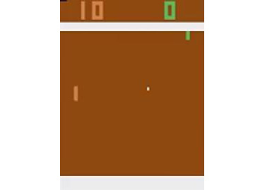
Figure 4.12: One frame of the Pong game
OpenAI Gym will be used to create the environment, while the OpenAI Baselines module will be used to train a custom policy network using the PPO algorithm.
As we saw in Exercise 4.04, Solving the CartPole Environment with the PPO Algorithm, both the custom approach, that is, using specific OpenAI modules, and the simple one, that is, using the built-in general command-line interface, will be implemented (in steps 1 to 5 and step 6, respectively).
Note
In order to run this exercise, you will need to install OpenAI Baselines. Please refer to the preface for the installation instructions.
In order to properly train the RL agent, many episodes are needed, so the training phase may take several hours to complete. A set of weights you can use for a pretrained agent has been provided at this address: https://packt.live/2XSY4yz. Use them to see the trained agent in action.
The following steps will help you complete this activity:
- Import all the required modules from OpenAI Baselines and TensorFlow in order to use the PPO algorithm.
- Define and register a custom convolutional neural network for the policy network.
- Create a function to build the environment in the format required by OpenAI Baselines.
- Build the PongNoFrameskip-v4 environment, choose the required policy network parameters, and train it.
- Run the trained agent in the environment and print the cumulative reward.
- Use the built-in OpenAI Baselines run script to train PPO on the PongNoFrameskip-v0 environment.
- Use the built-in OpenAI Baselines run script to run the trained model on the PongNoFrameskip-v0 environment.
- Use the pretrained weights provided to see the trained agent in action.
At the end of this activity, the agent is expected to easily win most of the time.
The final score of the agent should be like the one represented in the following frame most of the time:
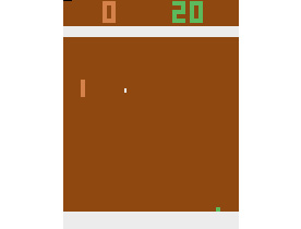
Figure 4.13: One frame of the real-time environment, after rendering
Note
The solution to this activity can be found on page 704.
Summary
This chapter introduced us to the key technologies and concepts we can use to get started with reinforcement learning. The first two sections described two OpenAI Tools, OpenAI Gym and OpenAI Universe. These are collections that contain a large number of control problems that cover a broad spectrum of contexts, from classic tasks to video games, from browser usage to algorithm deduction. We learned how the interfaces of these environments are formalized, how to interact with them, and how to create a custom environment for a specific problem. Then, we learned how to build a policy network with TensorFlow, how to feed it with environment states to retrieve corresponding actions, and how to save the policy network weights. We also studied another OpenAI resource, Baselines. We solved problems that demonstrated how to train a reinforcement learning agent to solve a classic control task. Finally, using all the elements introduced in this chapter, we built an agent and trained it to play a classic Atari video game, thus achieving better-than-human performance.
In the next chapter, we will be delving deep into dynamic programming for reinforcement learning.