3. Deep Learning in Practice with TensorFlow 2

Overview

This chapter will introduce you to TensorFlow and Keras and provide an overview of their key features and applications, as well as how they work in synergy. You will be able to implement a deep neural network with TensorFlow by addressing the main topics, from model creation, training, and validation, to testing. You will perform a regression task and solve a classification problem, thereby gaining hands-on experience with the frameworks. Finally, you will build and train a model to classify clothes images with high accuracy. By the end of this chapter, you will be able to design, build, and train deep learning models using the most advanced machine learning frameworks available.

Introduction

In the previous chapter, we covered the theory behind Reinforcement Learning (RL), explaining topics such as Markov chains and Markov Decision Processes (MDPs), Bellman equations, and a number of techniques we can use to solve MDPs. In this chapter, we will be looking at deep learning methods, all of which will play a primary role in building approximate functions for reinforcement learning. Specifically, we will look at different families of deep neural networks: fully connected, convolutional, and recurrent networks. These algorithms have the key capability of encoding knowledge that's been learned through examples in a compact and effective representation. In RL, they are typically used to approximate the so-called policy functions and value functions, which encode how the RL agent chooses its action, given the current state and the value associated with the current state, respectively. We will study the policy and value functions in the upcoming chapters.

Data is the new oil: This famous quote is being heard more and more frequently these days, especially in tech and economic industries. With the great amount of data available today, techniques to leverage such enormous quantities of information, thereby creating value and opportunities, are becoming key competitive factors and skills to have. All products and platforms that are provided to users for free (from social networks to apps related to wearable devices) use data that is provided by the users to generate revenues: think about the huge quantity of information they collect every day relating to our habits, preferences, or even body weight trends. These provide high-value insights that can be leveraged by advertisers, insurance companies, and local businesses to improve their offers so that they fit the market.

Thanks to the relevant increase in computational power availability and theory breakthroughs such as backpropagation-based training, deep learning has seen an explosion in the last 10 years, achieving unprecedented results in many fields, from image processing to speech recognition to natural language processing and understanding. In fact, it is now possible to successfully train large and deep neural networks by leveraging huge amounts of data and overcoming practical roadblocks that impeded their adoption in past decades. These models demonstrated the capability to exceed human performances in terms of both speed and accuracy. This chapter will teach you how to adopt deep learning to solve real-world problems by taking advantage of the top machine learning frameworks. TensorFlow and Keras, are the de facto production standards in the industry. Their success is mainly related to two aspects: TensorFlow's unrivaled performance in production environments in terms of both speed and scalability, and Keras' ease of use, which provides a very powerful, high-level interface that can be used to create deep learning models.

Now, let's take a look at the frameworks.

An Introduction to TensorFlow and Keras

In this section, both frameworks will be presented, thus providing you with a general overview of their architecture, the fundamental elements they are composed of, and listing some of their typical applications.

TensorFlow

TensorFlow is an open source numerical computation software library that leverages data flow computational graphs. Its architecture allows users to run it on a wide variety of hardware: from CPUs to Tensor Processing Units (TPUs), including GPUs as well as mobile and embedded platforms. The main difference between the three is the speed and the type of data they are able to perform computations with (multiplications and additions), which, of course, is of primary importance when aiming for maximum performance.

Note

We will be looking at various code implementation examples for TensorFlow in the Keras section of this chapter.

You can refer to the official documentation of TensorFlow for more information here: https://www.tensorflow.org/

The following article is a very good reference if you wish to find out more about the differences between GPUs and TPUs: https://iq.opengenus.org/cpu-vs-gpu-vs-tpu/

TensorFlow is based on a high-performance core implemented in C++ that's provided by a distributed execution engine that works as an abstraction toward the many devices it supports. We will be using TensorFlow 2, which has recently been released. It represents a major milestone for TensorFlow. Its main differences with respect to version 1 are related to its greater ease of use, in particular for model building. In fact, Keras has become the lead tool that's used to easily create models and experiment with them. TensorFlow 2 uses eager execution by default. This allowed the creators of TensorFlow to eliminate the previous complex workflow, which was based on the construction of a computational graph that's then run in a session. With eager execution, this is no longer required. Finally, the data pipeline has been simplified by means of the TensorFlow dataset, which is a common interface that's used to ingest standard or custom datasets with no need to define placeholders.

The execution engine is then interfaced with Python and C++ frontends, which, in turn, are the basis for the Layers API, which provides a simple interface for common layers in deep learning models. This hierarchical structure continues with higher-level APIs, including Keras (which we will describe later in this section). Finally, a set of common models are provided and can be used out of the box.

The following diagram provides an overview of how different TensorFlow modules are hierarchically organized, starting from the low level (bottom) up to the highest level (top):

Figure 3.1: TensorFlow architecture

The historical execution model of TensorFlow was based on computational graphs. Using this approach, the first step when building a model is to create a computation graph that fully describes the calculations we want to perform. The second step is to execute it. This approach has the drawback of being less intuitive with respect to common implementations, where the graph doesn't have to be completed before it can be executed. At the same time, it provides several advantages, making the algorithm highly portable, deployable on different types of hardware platforms, and capable of running in parallel on multiple instances.

In the latest version of TensorFlow (starting with v. 1.7), a new execution model called "eager execution" has been introduced. This is an imperative style for writing code. With eager execution enabled, all algorithmic operations can be run immediately, with no need to build a graph first and then execute it. This new approach has been greeted with enthusiasm and has some very important pros: first, it is much simpler to inspect and debug algorithms and access intermediate values; it is possible to directly use a Python control flow inside TensorFlow APIs; and it makes building and training complex algorithms very easy.

In addition, once the model that has been created using eager execution satisfies requirements, it is possible to automatically convert it into a graph, which makes it possible to leverage all the advantages we looked at previously, such as saving, porting, and distributing models optimally.

Like other machine learning frameworks, TensorFlow provides a large number of ready-to-use models and for many of them, it also provides trained model weights along with the model graph, meaning we can run such models out of the box, and even tune them for a specific use case to take advantage of techniques such as transfer learning with fine tuning. We will cover these in the following sections.

The models provided cover a wide range of different applications, for example:

• Image classification: Able to classify images into categories.
• Object detection: Capable of detecting and localizing multiple objects in images.
• Language understanding and translation: Performing natural language processing for tasks such as word prediction and translation.
• Patch harmonization and style transfer: The algorithm is able to apply a given style (represented, for example, through a painting) to a given photo (refer to the following example).

As we mentioned previously, many of the models include trained weights and examples explaining how to use them. Thus, it is very straightforward to adopt "transfer learning," that is, to take advantage of these pretrained models by creating new ones, retraining only a part of the network on a new dataset. This can be significantly smaller with respect to the one used to train the entire network from scratch.

TensorFlow models can also be deployed on mobile devices. After being trained on large systems, they are optimized to reduce their footprint, which cannot be too big to meet platform limitations. For example, the TensorFlow project known as MobileNet is developing a set of computer vision models specifically designed with optimal speed/accuracy trade-offs in mind. These are typically considered for embedded devices and mobile applications.

The following image represents a typical example of an object detection application where the input image is processed and three objects have been detected, localized, and classified:

Figure 3.2: Object detection

The following image shows how style transfer works: the style of the famous painting "The Great Wave off Kanagawa" has been applied to a photo of the Seattle skyline. The results keep the key parts of the picture (the majority of the buildings are there, mountains, and so on), but it is represented through stylistic elements that have been extrapolated from the reference image:

Figure 3.3: Style transfer

Now, let's learn about Keras.

Keras

Building deep learning models is quite complex, especially when we have to deal with all the typical low-level aspects of major frameworks, and this is one of the most relevant barriers for newcomers in the machine learning field. As an example, the following code shows how to create a simple neural network (one hidden layer with an input size of 100 and an output size of 10) with a low-level TensorFlow API.

In the following code snippet, two functions are being defined. The first builds the weights matrix of a network layer, while the second one creates the bias vector:

def weight_variable(shape):

    shape = tf.TensorShape(shape)

    initial_values = tf.truncated_normal(shape, stddev=0.1)

    return tf.Variable(initial_values)

def bias_variable(shape):

    initial_values = tf.zeros(tf.TensorShape(shape))

    return tf.Variable(initial_values)

Next, the placeholders for the input (X) and labels (y) are created. They will contain the training samples that will be used to fit the model:

# Define placeholders

X = tf.placeholder(tf.float32, shape=[None, 100])

y = tf.placeholder(tf.int32, shape=[None, 10])

Two matrices and two vectors are created, one couple for each of the two hidden layers of the network to be created, with the functions previously defined. These will contain trainable parameters (network weights):

# Define variables

w1 = weight_variable([X_input.shape[1], 64])

b1 = bias_variable([64])

w2 = weight_variable([64, 10])

b2 = bias_variable([10])

The two network layers are defined via their mathematical definition: matrix multiplication, plus the bias sum and activation function applied to the result:

# Define network

# Hidden layer

z1 = tf.add(tf.matmul(X, w1), b1)

a1 = tf.nn.relu(z1)

# Output layer

z2 = tf.add(tf.matmul(a1, w2), b2)

y_pred = tf.nn.softmax(z2)

y_one_hot = tf.one_hot(y, 10)

The loss function is defined, the optimizer is initialized, and the training metrics are chosen. Finally, the graph is run to perform training:

# Define loss function

loss = tf.losses.softmax_cross_entropy(y, y_pred,

       reduction=tf.losses.Reduction.MEAN)

# Define optimizer

optimizer = tf.train.AdamOptimizer(0.01).minimize(loss)

# Metric

accuracy = tf.reduce_mean(tf.cast(tf.equal(tf.argmax(y, axis=1),

           tf.argmax(y_pred, axis=1)), tf.float32))

for _ in range(n_epochs):

    sess.run(optimizer, feed_dict={X: X_train, y: y_train})

As you can see, we need to manually manage many different aspects: variable declaration, weights initialization, layer creation, layer-related mathematical operations, and the definition of the loss function, optimizers, and metrics. For comparison, the same neural network will be created using Keras later in this section.

Note

The preceding code snippet is an example that demonstrates how to implement a simple fully connected neural network with a TensorFlow low-level API. In Exercise 3.01, Building a Sequential Model with the Keras High-Level API, you will see how much more straightforward it is to do the same job using a Keras high-level API.

Among many different proposals, Keras has become one of the main references for high-level APIs, especially the context of those targeted at creating neural networks. It is written in Python and can be interfaced with different backend computation engines, one of which is, of course, TensorFlow.

Note

You can refer to the official documentation for further reading on Keras here: https://keras.io/.

Keras' conception has been driven by some clear principles, in particular, modularity, user friendliness, easy extendibility, and its straightforward integration with Python. Its aim is to favor adoption by newcomers and non-experienced users, and it presents a very gentle learning curve. It provides many different standalone modules, ranging from neural network layers to optimizers, from initialization schemes to cost functions. These can be easily created to create deep learning models quickly and to code them directly in Python, with no need to use separate configuration files. Given these features, its wide adoption, the fact that it can be interfaced with a large number of different backend engines (for example, TensorFlow, CNTK, Theano, MXNet, and PlaidML) and its wide choice of deployment options, it has risen to become the standard choice in the field.

Since it doesn't have its own low-level implementation, Keras needs to rely on an external element. This can be easily modified by editing (for Linux users) the $HOME/.keras/keras.json file, where it is possible to specify the backend name. It is also possible to specify it by means of the KERAS_BACKEND environment variable.

Keras' fundamental class is Model. There are two different types of model available: The sequential model (which we will use extensively), and the Model class, which is used with the functional API.

The sequential model can be seen as a linear stack of layers, piled one after the other in a very simple way, and these layers can be described very easily. The following exercise shows how short a Python script in Keras that builds a deep neural network using model.add() can be in order to define two dense layers in a sequential model.

Exercise 3.01: Building a Sequential Model with the Keras High-Level API

This exercise shows how to easily build a sequential model, composed of two dense layers, with the Keras high-level API, step by step:

1. Import the TensorFlow module and print its version:

   import tensorflow as tf

   from __future__ import absolute_import, division,

   print_function, unicode_literals

   import tensorflow as tf

   print("TensorFlow version: {}".format(tf.__version__))

   This outputs the following line:

   TensorFlow version: 2.1.0

2. Build the model using Keras' sequential and add methods and print a network summary. To continue in parallel with a low-level API, the same activation functions are used. We are using ReLu here, which is a typical activation function that's used for hidden layers. It is a key element that provides nonlinearity to the model thanks to its nonlinear shape. We also use Softmax, which is the activation function typically used for output layers in classification problems. It receives the output values (so-called "logits") from the previous layer and performs a weighting of them, defining all the probabilities of the output classes. The input_dim is the dimension of the input feature vector; it is assumed to have a dimension of 100:

   model = tf.keras.Sequential()

   model.add(tf.keras.layers.Dense(units=64,

                                   activation='relu', input_dim=100))

   model.add(tf.keras.layers.Dense(units=10, activation='softmax'))

3. Print the standard model architecture:

   model.summary()

   In our case, the network model summary is as follows:

   Model: "sequential_1"

   _________________________________________________________________

   Layer (type) Output Shape Param #

   =================================================================

   dense_2 (Dense) (None, 64) 6464

   _________________________________________________________________

   dense_3 (Dense) (None, 10) 650

   =================================================================

   Total params: 7,114

   Trainable params: 7,114

   Non-trainable params: 0

   _________________________________________________________________

   The preceding output is a useful visualization that gives us a clear understanding of layers, their type and shape, and the number of network parameters.

   Note

   To access the source code for this specific section, please refer to https://packt.live/30A9Dw9.

   You can also run this example online at https://packt.live/3cT0cKL.

As anticipated, this exercise showed us how to create a sequential model and how to add two layers to it in a very straightforward way.

We will deal with the remaining aspects later on, but it is still worth noting that training the model we just created and performing inference only requires very few lines of code, as presented in the following snippet, which needs to be appended to the snippet of Exercise 3.01, Building a Sequential Model with the Keras High-Level API:

model.compile(loss='categorical_crossentropy', optimizer='sgd',

              metrics=['accuracy'])

model.fit(x_train, y_train, epochs=5, batch_size=32)

loss_and_metrics = model.evaluate(x_test, y_test, batch_size=128)

classes = model.predict(x_test, batch_size=128)

If more complex models are required, the sequential API is too limited. For these needs, Keras provides the functional API, which allows us to create models that are able to manage complex networks graphs, such as networks with multiple inputs and/or multiple outputs, recurrent neural networks where data processing is not sequential but instead is cyclic, and context, where layers' weights are shared among different parts of the network. For this purpose, Keras allows us to leverage the same set of layers as the sequential model, but provides more flexibility in putting them together. First, we have to define the layers and put them together. An example is presented in the following snippet.

First, after importing TensorFlow, an input layer of dimension 784 is created:

import tensorflow as tf

inputs = tf.keras.layers.Input(shape=(784,))

Inputs are processed by the first hidden layer. They go through the ReLu activation function and are returned as output. This output then becomes the input for the second hidden layer, which is exactly the same as the first one, and returns another output, again stored in the x variable:

x = tf.keras.layers.Dense(64, activation='relu')(inputs)

x = tf.keras.layers.Dense(64, activation='relu')(x)

Finally, the x variable goes as input to the final output layer, which has a softmax activation function, and returns predictions:

predictions = tf.keras.layers.Dense(10, activation='softmax')(x)

Once all the passages have been completed, the model can be created by telling Keras where it starts (input variable) and where it ends (predictions variable):

model = tf.keras.models.Model(inputs=inputs, outputs=predictions)

After the model has been built, it is compiled by specifying the optimizer, the loss, and the metrics. Finally, it is fitted onto the training data:

model.compile(optimizer='rmsprop',

              loss='categorical_crossentropy',

              metrics=['accuracy'])

model.fit(data, labels) # starts training

Keras provides a large number of predefined layers, as well as the possibility to code custom ones. Among those, the following are the already available layers:

• Dense layers, which are typically used for fully connected neural networks. They consist of a matrix of weights and a bias.
• Convolution layers are filters that are defined by specific kernels, which are then convolved with the inputs they are applied to. There are layers available for different input dimensions, from 1D to 3D, including the possibility to embed in them complex operations, such as cropping or transposition.
• Locally connected layers are similar to convolution layers in the sense that they act only on a subgroup of the input features, but, unlike convolution layers, they don't share weights.
• Pooling layers are layers that are used to downscale the input. As convolutional layers, they are available for inputs with dimensionality ranging from 1D to 3D. They include most of the common variants, such as max and average pooling.
• Recurrent layers are used for recurrent neural networks, where the output of a layer is also fed backward in the network. They support state-of-the-art units such as Gated Recurrent Units (GRUs), Long Short-Term Memory (LSTM) units, and others.
• Activation functions are also available in the form of layers. These are functions that are applied to layer outputs, such as ReLu, Elu, Linear, Tanh, and Softmax.
• Lambda layers are layers for embedding arbitrary, user-defined expressions.
• Dropout layers are special objects that randomly set a fraction of the input units to 0 at each training update to avoid overfitting (more on this later).
• Noise layers are additional layers, such as dropout, that are used to avoid overfitting.

Keras also provides common datasets, as well as famous models. For image-related applications, many networks are available, such as Xception, VGG16, VGG19, ResNet50, InceptionV3, InceptionResNetV2, MobileNet, DenseNet, NASNet, and MobileNetV2TK, all of which are pretrained on ImageNet. Keras also provides text and sequences and generative models, making a total of more than 40 algorithms.

As we saw for TensorFlow, Keras models have a vast choice of deployment platforms, including iOS, via CoreML (supported by Apple); Android, via the TensorFlow Android runtime; in a browser, via Keras.js and WebDNN; on Google Cloud, via TensorFlow-Serving; in a Python webapp backend; on the JVM, via DL4J model import; and on a Raspberry Pi.

Now that we've looked at both TensorFlow and Keras, from the next section onward, our main focus will be on how to use them in combination to create deep neural networks. Keras will be used as a high-level API, given its user-friendliness, including TensorFlow, which will be the backend.

How to Implement a Neural Network Using TensorFlow

In this section, we will look at the most important aspects to consider when implementing a deep neural network. Starting with the very basic concepts, we will go through all the steps that lead up to the creation of a state-of-the-art deep learning model. We will cover the network architecture's definition, training strategies, and performance improvement techniques, understanding how they work, and preparing you so that you can tackle the next section's exercises, where these concepts will be applied to solve real-world problems.

To successfully implement a deep neural network in TensorFlow, we have to complete a given number of steps. These can be summarized and grouped as follows:

1. Model creation: Network architecture definition, input features encoding, embeddings, output layers
2. Model training: Loss function definition, optimizer choice, features normalization, backpropagation
3. Model validation: Strategies and key elements
4. Model improvement: Overfitting countermeasures
5. Model test and inference: Performance evaluation and online predictions

Let's look at each of these steps in detail.

Model Creation

The very first step is to create a model. Choosing an architecture is hardly something that can be done a priori on paper. It is a typical process that requires experimentation, going back and forth between model design and field validation and testing. This is the phase where all network layers are created and properly linked to generate a complete processing operation set that goes from inputs to outputs.

The very first layer is the one that is interfaced with input data, specifically, the so-called "input features." In the case of images, for example, input features are image pixels. Depending on the nature of the layer, the input features' dimensionality needs to be taken into account. You will learn how to choose layer dimensions, depending on the layer's nature, in the upcoming sections.

The very last layer is called the output layer. It generates model predictions, so its dimensions depend on the nature of the problem. For example, in classification problems, where the model has to predict in which of the, say, 10 classes a given instance falls, the model will have 10 neurons in the output layer providing 10 scores (one per class). In the upcoming sections, we will illustrate how to create output layers with the correct dimensions.

Between the first and last layers, there are intermediate layers, called hidden layers. These layers constitute the network architecture, and they are responsible for the core processing capabilities of the model. At the time of writing, a rule that can be used to choose the best network architecture doesn't exist; this is a process that requires a lot of experimentation, under the guidance of some general principles.

A very powerful and common approach is to leverage proven models from academic papers, using them as a starting point, and then adjusting the architecture appropriately to fit and fine-tune it to the custom problem. When pretrained literature models are used and fine-tuned, the procedure is called "transfer learning," meaning we are leveraging an already trained model and transferring its knowledge to the new model, which then won't start from scratch.

Once the model has been created, all its parameters (weights/biases) must be initialized (for all non-pretrained layers). You might be tempted to set them all equal to zero, but this is hardly a good choice. There are many different initialization schemes available, and again, which one to choose requires experience and experimentation. This aspect will become clearer in the following sections. Implementation will rely on default initialization to be performed by Keras/TensorFlow, which is usually a good and safe starting point.

A typical code example for model creation can be seen in the following snippet, which we studied in the previous section:

inputs = tf.keras.layers.Input(shape=(784,))

x = tf.keras.layers.Dense(64, activation='relu')(inputs)

x = tf.keras.layers.Dense(64, activation='relu')(x)

predictions = tf.keras.layers.Dense(10, activation='softmax')(x)

model = tf.keras.models.Model(inputs=inputs, outputs=predictions)

Model Training

When a model is initialized and applied to input data without undergoing a training phase, it outputs random values. In order to improve its performance, we need to adjust its parameters (weights) to minimize its errors. This is the aim of the model training stage, which requires the following steps:

1. First, we have to evaluate how "wrong" the model is with a given parameter configuration by computing a so-called "loss," which is a measure of model prediction error.
2. Second, a hyperdimensional gradient is computed, which tells us how (in which direction) the model needs to change its parameters in order to improve current performance, thereby minimizing the loss function (it is indeed an optimization process).
3. Finally, the model parameters are updated by taking a "step" in the negative gradient direction (following some precise rules) and the whole process restarts from the loss evaluation stage.

This procedure is repeated as many times as needed until the system converges and the model reaches its maximum performance (minimum loss).

A typical code example for model training is shown in the following snippet, which we studied in the previous sections:

model.compile(optimizer='rmsprop',

              loss='categorical_crossentropy',

              metrics=['accuracy'])

model.fit(data, labels) # starts training

Loss Function Definition

Model error can be measured by means of different loss functions. How to choose the best one requires experience. For complex applications, we often need to carefully adapt the loss function in order to drive training in directions we are interested in. As an example, let's look at how to define a typical loss that's used for classification problems: the sparse categorical cross entropy. To create it in Keras, we can use the following instruction:

loss_CatCrossEntropy = tf.keras.losses

                       .SparseCategoricalCrossentropy()

This function operates on two inputs: true labels and predicted labels. Based on their values, it computes the loss associated with the model:

loss_CatCrossEntropy(y_true=groundTruth, y_pred=predictions)

Optimizer Choice

The second and third steps, estimating the gradient and updating the parameters, respectively, are addressed by optimizers. These objects calculate gradients and perform update steps in the gradient's direction to minimize model loss. There are many optimizers available, from the simplest ones to the most advanced (refer to the following diagram). They provide different performances, and which one to select is, again, a matter of experience and a trial-and-error process. As an example, the following code selects the Adam optimizer, assigning a specific learning rate of 0.01. This parameter regulates how "large" the step taken will be along the gradient direction:

optimizer = tf.keras.optimizers.Adam(learning_rate=0.01)

optimizer = tf.keras.optimizers.Adadelta(learning_rate=0.01)

optimizer = tf.keras.optimizers.Adagrad(learning_rate=0.01)

optimizer = tf.keras.optimizers.Adamax(learning_rate=0.01)

optimizer = tf.keras.optimizers.Ftrl(learning_rate=0.01)

optimizer = tf.keras.optimizers.Nadam(learning_rate=0.01)

optimizer = tf.keras.optimizers.RMSprop(learning_rate=0.01)

optimizer = tf.keras.optimizers.SGD(learning_rate=0.01)

The following diagram is an instantaneous snapshot comparing different optimizers. It shows how quickly they move toward the minimum, starting all at the same time. We can see how some of them are faster than others:

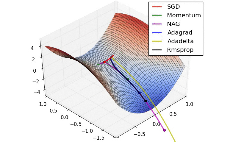
Figure 3.4: Comparison of optimizer minimization steps

Note

The preceding diagram was created by Alec Radford (https://twitter.com/alecrad).

Learning Rate Scheduling

In most cases, and for most deep learning models, the best results are achieved if the learning rate is gradually reduced during training. The reason for this can be seen in the following diagram:

Figure 3.5: Optimization behavior when using different learning rate values

When approaching the minimum of the loss function, we want to take smaller and smaller steps to efficiently reach the very bottom of the hyperdimensional concavity.

With Keras, it is possible to prescribe many different decreasing functions for the learning rate trend over epochs by means of a scheduler. One common choice is InverseTimeDecay. This can be implemented as follows:

lr_schedule = tf.keras.optimizers.schedules

              .InverseTimeDecay(0.001,

                                decay_steps=STEPS_PER_EPOCH*1000,

                                decay_rate=1, staircase=False)

The preceding code sets a decreasing function through InverseTimeDecay to hyperbolically decrease the learning rate to 1/2 of the base rate at 1,000 epochs, 1/3 at 2,000 epochs, and so on. This can be seen in the following graph:

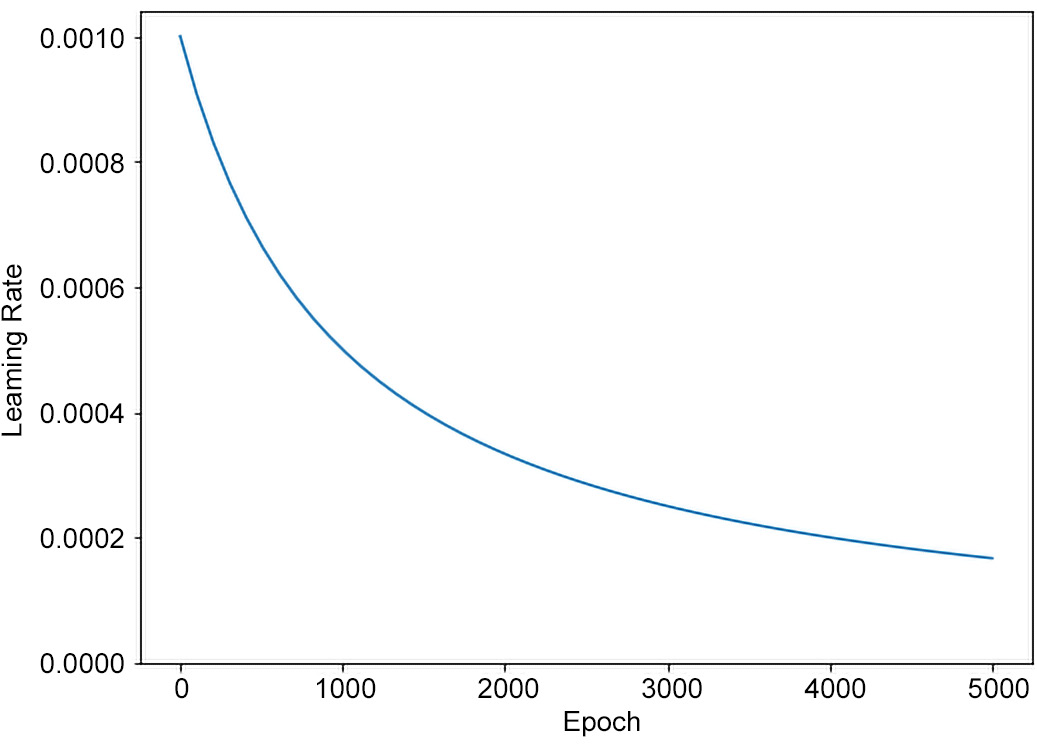
Figure 3.6: Inverse time decay learning rate scheduling

Then, it is applied to an optimizer as an argument, as shown in the following snippet for the Adam optimizer:

tf.keras.optimizers.Adam(lr_schedule)

Each optimization step makes the loss drop, thereby improving the model. It is then possible to repeat the same process over and over until convergence is reached and the loss stops decreasing. The number of optimization steps performed is usually called the number of epochs.

Feature Normalization

The broad applications for deep neural networks favor their usage on very different types of inputs, from image pixels to credit card transaction history, from social account profile habits to audio recordings. From this, it is clear that raw input features cover very different numerical scales. As mentioned previously, training these models requires solving an optimization problem using a loss gradient calculation. For this reason, numerical aspects are of paramount importance, resulting in a speeding up of the process, as well as making it more robust. One of the most important practices, in this context, is feature normalization or standardization. The most common approach consists of performing the following steps for each feature:

1. Calculating the mean and standard deviation using all the training set instances.
2. Subtracting the mean and dividing by standard deviation. Values calculated on the training set must be applied to the training, validation, and test sets.

This way, all the features will have zero mean and standard deviation equal to 1. Different, but similar, approaches scale feature values between a user-defined minimum-maximum range (for example, between –1 and 1) or apply similar transformations (for example, log scaling). As usual, in the field, which approach works better is hardly predictable and requires experience and a trial-and-error approach.

The following code snippet shows how data normalization is performed, wherein the mean and standard deviation of the original values are calculated, the mean is then subtracted from the original values, and the result is then divided by the standard deviation:

train_stats = train_dataset.describe()

train_stats = train_stats.transpose()

def norm(x):

    return (x - train_stats['mean']) / train_stats['std']

normed_train_data = norm(train_dataset)

Model Validation

As stated in the previous subsections, a large portion of choices require experimentation, meaning we have to select a given configuration and evaluate how the corresponding model performs. In order to compute this performance measure, the candidate model must be applied to a set of instances and its output compared against ground truth values. This step can be repeated many times, depending on how many alternative configurations we want to compare. In the long run, these configuration choices can suffer an excessive influence of the set of instances used to measure model performance. For this reason, in order to have a final accurate performance measure of the model of choice, it has to be tested on a new set of instances that have never been seen before. The first set of instances is called a "validation set," while the final one is called a "test set."

There are different choices we can adopt when defining training, validation, and test sets, such as the following:

• 70:20:10: The initial dataset is decomposed into three chunks, that is, the training, validation, and test sets, with the proportion 70:20:10, respectively.
• 80:20 + k-Folding: The initial dataset is decomposed into two chunks, 80% training and 20% testing, respectively. Validation is performed using k-Folding on the training dataset: it is divided into 'k' folds and, in turn, training is carried out in 'k-1' folds, while validation is performed on the k-th piece. 'K' varies from 1 to k and metrics are averaged to obtain a global measure.

Many variants of the preceding methods can be used. The choices are strictly related to the problem and the available dataset.

The following code snippet shows how to prescribe an 80:20 split for validation when fitting a model on a training dataset:

model.fit(normed_train_data, train_labels, epochs=epochs,

          validation_split = 0.2, verbose=2)

Performance Metrics

In order to measure performances, beside the loss functions, other metrics are usually adopted. There is a very wide set of metrics available, and the question as to which you should use depends on many factors, including the type of problem, dataset characteristics, and so on. The following is a list of the most common ones:

• Mean Squared Error (MSE): Used for regression problems.
• Mean Absolute Error (MAE): Used for regression problems.
• Accuracy: Number of correct predictions divided by the number of total tested instances. This is used for classification problems.
• Receiver Operating Characteristic Area Under Curve (ROC AUC): Used for binary classification, especially in the presence of highly unbalanced data.
• Others: Fβ score, precision, and recall.

Model Improvement

In this section, we will look at a few techniques that can be used to improve the performance of a model.

Overfitting

A common problem we may typically encounter when training deep neural networks is a critical drop in model performance (measured, of course, on the validation or test set) when the number of training epochs passes a given threshold, even if, at the same time, the training loss continues to decrease. This phenomenon is called overfitting. It can be defined as follows: a highly representative model, a model with the relevant number of degrees of freedom (for example, a neural network with many layers and neurons), if trained "too much," bends itself to adhere to the training data, with the intent to minimize the training loss. This results in poor generalization performances, making validation and/or test errors higher. Deep learning models, thanks to their high-dimensional parameter space, are usually very good at fitting the training data, but the actual aim of building a machine learning model is being able to generalize what has been learned, not merely fit a dataset.

At this point, we might be tempted to significantly reduce the number of model parameters to avoid overfitting. But this would cause different problems. In fact, a model with an insufficient number of parameters would incur underfitting. Basically, it would not be able to properly fit the data, again resulting in poor performance, this time on both the training and validation/test sets.

The correct solution is the one that finds a proper balance between having a large number of parameters that would perfectly fit training data and having too small a number of model degrees of freedom, resulting in it being able to capture important information from data. It is currently not possible to identify the right size for a model so that it won't face overfitting or underfitting problems. Experimentation is a key element in this regard, thereby requiring the data engineer to build and test different architectures. A good rule is to start with models with a relatively small number of parameters and then increase them until generalization performance grows.

The best solution against overfitting is to enrich the training dataset with new data. Aim for complete coverage of the full range of inputs that are supported and expected by the model. New data should also contain additional information with respect to starting the dataset in order to effectively contrast overfitting and to result in a better generalization error. When collecting additional data is not possible or too expensive, it is necessary to adopt specific, very powerful techniques. The most important ones will be described here.

Regularization

Regularization is one of the most powerful tools used to contrast overfitting. Given a network architecture and a set of training data, there is an entire space of possible weights that produce the same results. Every combination of weights in this space defines a specific model. As we saw in the preceding section, we have to prefer, as a general principle, simple models over complex ones. A common way to reach this goal is to force network weights to assume small values, thereby regularizing the distribution of weights. This can be achieved through "weight regularization". This consists of shaping the loss function so that it can take weight values into consideration, adding a new term to it that is directly proportional to their magnitude. Two approaches are usually encountered:

• L1 regularization: The term that's added to the loss function is proportional to the absolute value of the weight coefficients, commonly referred to as the "L1 norm" of the weights.
• L2 regularization: The term that's added to the loss function is proportional to the square of the value of the weight coefficients, commonly referred to as the "L2 norm" of the weights.

Both of these have the effect of limiting the magnitude of the weights, but while L1 regularization tends to drive weights toward exactly zero, L2 regularization penalizes weights with a less strict constraint since the additional loss term grows at a higher rate. L2 is, in general, more common.

Keras contains pre-built L1 and L2 regularization objects. The user has to pass them as arguments to the network layers that they want to apply the technique to. The following code shows how to apply it to a common dense layer:

tf.keras.layers.Dense(512, activation='relu',

                      kernel_regularizer=tf.keras

                                         .regularizers.l2(0.001))

The parameter that was passed to the L2 regularizer (0.001) shows that an additional loss term equal to 0.001 * weight_coefficient_value**2 will be added to the total loss of the network for every coefficient in the weight matrix.

Early Stopping

Early stopping is a specific form of regularization. The idea is to keep track of both training and validation errors during training and to continue training the model until both training and validation losses decrease. This allows us to spot the epochs threshold, after which the training loss' decrease would come as an expense of increased generalization error, so that we can stop training when validation/test performances have reached their maximum. One typical parameter the user has to choose when adopting this technique is the number of epochs the system should wait for and monitor before stopping the iterations if no improvement in the validation error is shown. This parameter is commonly named "patience."

Dropout

One of the most popular and effective reliable regularization techniques for neural networks is Dropout. It was developed at the University of Toronto by Prof. Hinton and his research group.

When Dropout is applied to a layer, a certain percentage of the layer output features during training are randomly set to zero (they drop out). For example, if the output of a given layer would normally have been [0.3, 0.4, 1.2, 0.1, 1.5] for a given set of input features during training, when dropout is applied, the same output vector will have some zero entries randomly distributed; for example, [0.3, 0, 1.2, 0.1, 0].

The idea behind dropout is to encourage each node to output values that are highly informative and meaningful on their own, without relying on its neighboring ones.

The parameter to be set when inserting a dropout layer is called the dropout rate: this represents the fraction of features that are being set to zero and is usually chosen in a range between 0.2 and 0.5. When performing inference, dropout is deactivated, and an additional operation needs to be executed to take into account the fact that more units will be active with respect to training time. To re-establish a balance between these two situations, the layer's output values are multiplied by a factor equal to the dropout rate, resulting in a scaling-down operation. In Keras, dropout can be introduced in a network using the dropout layer, which is applied to the output of the layer immediately before it. Consider the following code snippet:

dropout_model = tf.keras.Sequential([

    #[...]

    tf.keras.layers.Dense(512, activation='relu'),

    tf.keras.layers.Dropout(0.5),

    tf.keras.layers.Dense(256, activation='relu'),

    #[...]

    ])

As you can see, dropout is applied to the layer with 512 neurons, setting 50% of their values to 0.0 at training time, and multiplying their values by 0.5 at inference time.

Data Augmentation

Data augmentation is particularly useful when the number of instances available for training is limited. It is super easy to understand how it is implemented and works in the context of image processing. Suppose we want to train a network to classify images of different breeds of a specific species and we only have a limited number of examples for each breed. How can we enlarge the dataset to help the model generalize better? Data augmentation plays a major role in this context: the idea is to create new training instances, starting from those we already have and tweaking them appropriately. In the case of images, we can act on them by doing the following:

• Random rotations with respect to a point in the vicinity of the center
• Random crops
• Random affine transformations (shear, resize, and so on)
• Random horizontal/vertical flips
• White noise superimposition
• Salt and pepper noise superimposition

These are a few examples of data augmentation techniques that can be used for images, which, of course, have counterparts in other domains. This approach makes the model way more robust and improves its generalization performance, allowing it to abstract notions and knowledge about the specific problem it is facing in a more general way by giving privilege to the most informative input features.

Batch Normalization

Batch normalization is a technique that consists of applying a normalization transform to every batch of data. For example, in the context of training a deep network with a batch size of 128, meaning the system will process 128 training samples at a time, the batch normalization layer works this way:

1. It calculates the mean and variance for each feature using all the samples of the given batch.
2. It subtracts the corresponding feature mean that was previously calculated from each feature of every batch sample.
3. It divides each feature of every batch sample by the square root of the corresponding feature variance.

Batch normalization has many benefits. It was initially proposed to solve internal covariate shift. While training deep networks, the layer's parameters continuously change, causing internal layers to constantly adapt and readjust to new distributions they see as inputs coming from the preceding layers. This is particularly critical for deep networks, where small changes in the first layers are amplified through the network. Normalizing the layer's output helps in bounding these shifts, speeding up training and generating more reliable models.

In addition, using batch normalization, we can do the following:

• We can adopt a higher learning rate without the risk of incurring the problem of vanishing or exploding gradients.
• We can favor network regularization by making its generalization better and mitigating overfitting.
• We can make the model become more robust to different initialization schemes and learning rates.

Model Testing and Inference

Once the model has been trained and its validation performances are satisfactory, we can move on to the final stage. As already stated, a final, accurate, model performance estimation requires that we test the model on a set of instances it has never seen before: the test set. After performance has been confirmed, the model can be moved to production for online inference, where it will serve as designed: new instances will be provided to the model and it will output predictions, leveraging the knowledge it has been designed and trained to have.

In the following subsections, three types of neural networks with specific elements/layers will be described. They will provide straightforward examples of different technologies that are widely encountered in the field.

Standard Fully Connected Neural Networks

The term fully connected neural network is commonly used to indicate deep neural networks that are only composed of fully connected layers. Fully connected layers are the layers whose neurons are connected to all the neurons of the previous layer, as well as all the neurons of the next one, as shown in the following diagram:

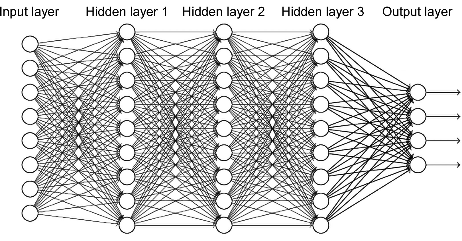
Figure 3.7: A fully connected neural network

This chapter will mainly deal with fully connected networks. They map inputs to outputs through a series of intermediate hidden layers. These architectures are capable of handling a wide variety of problems, but they are limited in terms of the input dimensions they can handle, as well as the number of layers and number of neurons, due to the rapid growth of the number of parameters, which is strictly dependent on these variables.

An example of a fully connected neural network that will be encountered later on is the one presented as follows, built with the Keras API. It connects an input layer who dimension is equal to len(train_dataset.keys()) to an output layer of dimension 1, by means of two hidden layers with 64 neurons each:

    model = tf.keras.Sequential([tf.keras.layers.Dense

            (64, activation='relu',

             input_shape=[len(train_dataset.keys())]),

             tf.keras.layers.Dense(64, activation='relu'),

             tf.keras.layers.Dense(1)])

Now, let's quickly solve an exercise in order to aid our understanding of fully connected neural networks.

Exercise 3.02: Building a Fully Connected Neural Network Model with the Keras High-Level API

In this exercise, we will build a fully connected neural network with an input dimension of 100, 2 hidden layers, and an output layer of 10 neurons. The following are the steps to complete this exercise:

1. Import the TensorFlow module and print its version:

   from __future__ import absolute_import, division,

   print_function, unicode_literals

   import tensorflow as tf

   print("TensorFlow version: {}".format(tf.__version__))

   This prints out the following line:

   TensorFlow version: 2.1.0

2. Create the network using the Keras sequential module. This allows us to build a model by stacking a series of layers, one after the other. In this specific case, we're using two hidden layers and an output layer:

   INPUT_DIM = 100

   OUTPUT_DIM = 10

   model = tf.keras.Sequential([tf.keras.layers.Dense

           (128, activation='relu',

           input_shape=[INPUT_DIM]),

           tf.keras.layers.Dense(256, activation='relu'),

           tf.keras.layers.Dense(OUTPUT_DIM, activation='softmax')])

3. Print the summary to look at the model description:

   model.summary()

   The output will be as follows:

   Model: "sequential"

   _________________________________________________________________

   Layer (type) Output Shape Param #

   =================================================================

   dense (Dense) (None, 128) 12928

   _________________________________________________________________

   dense_1 (Dense) (None, 256) 33024

   _________________________________________________________________

   dense_2 (Dense) (None, 10) 2570

   =================================================================

   Total params: 48,522

   Trainable params: 48,522

   Non-trainable params: 0

   _________________________________________________________________

As you can see, the model has been created and the summary provides us with a clear understanding of the layers, their types and shapes, and the number of parameters of the network, which is very useful when building neural networks in real life.

Note

To access the source code for this specific section, please refer to https://packt.live/37s1M5w.

You can also run this example online at https://packt.live/3f9WzSq.

Now, let's move on and understand convolutional neural networks.

Convolutional Neural Networks

The term Convolutional Neural Network (CNN) usually identifies a deep neural network composed of a combination of the following:

• Convolutional layers
• Pooling layers
• Fully connected layers

One of the most successful applications of CNNs is in image and video processing tasks. In fact, they are way more capable, with respect to fully connected ones, of handling high-dimensional inputs such as images. They are also widely used for anomaly detection tasks, being used in autoencoders, as well as encoders for reinforcement learning algorithms, specifically for policy and value networks.

Convolutional layers can be thought of as a series of filters applied (convolved) to layer inputs to generate layer outputs. The main parameters of these layers are the number of filters they have and the dimension of the convolution kernel.

Pooling layers reduce the dimensions of the data; they combine the outputs of neuron clusters at one layer into a single neuron in the next layer. Pooling layers may compute a max (MaxPooling), which uses the maximum value from each cluster of neurons at the prior layer, or an average (AveragePooling), which uses the average value from each cluster of neurons at the prior layer.

These convolution/pooling operations encode input information in a compressed representation, up to a point where these new deep features, also called embeddings, are typically provided as inputs to standard fully connected layers at the very end of the network. A classic convolutional neural network schematization is represented in the following figure:

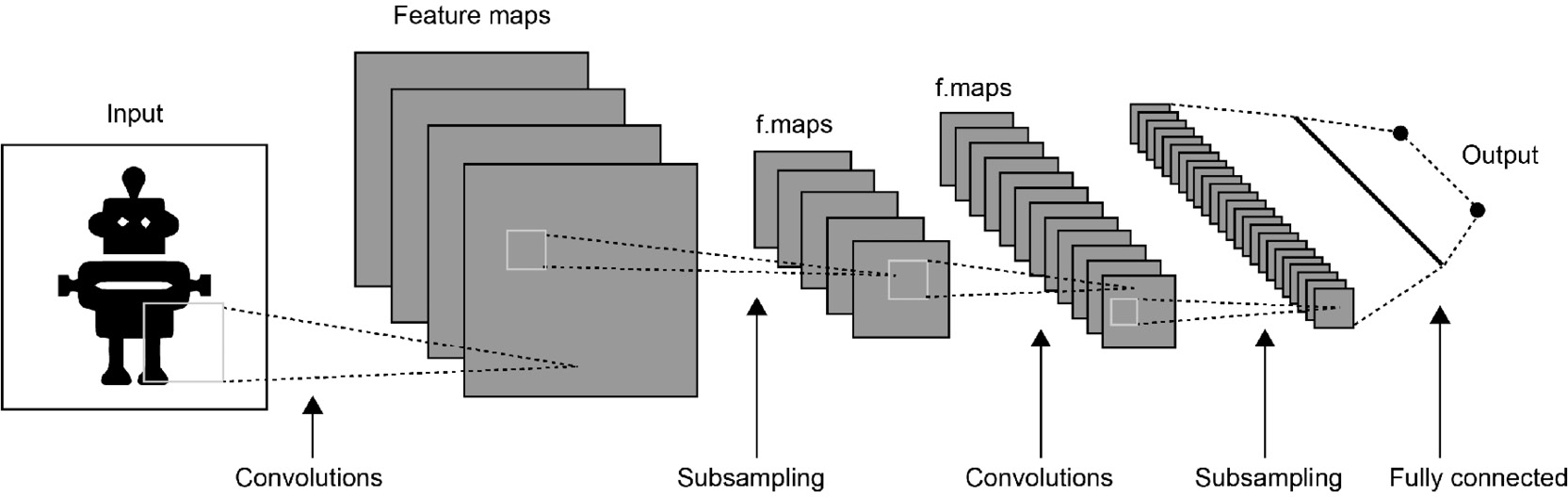
Figure 3.8: Convolutional neural network scheme

The following exercise shows how to create a convolutional neural network using the Keras high-level API.

Exercise 3.03: Building a Convolutional Neural Network Model with the Keras High-Level API

This exercise will show you how to build a convolutional neural network with three convolutional layers (number of filters equal to 16, 32, and 64, respectively, and a kernel size of 3), alternated with three MaxPooling layers, and, at the end, two fully connected layers with 512 and 1 neurons, respectively. Here is the step-by-step procedure:

1. Import the TensorFlow module and print its version:

   from __future__ import absolute_import, division,

   print_function, unicode_literals

   import tensorflow as tf

   print("TensorFlow version: {}".format(tf.__version__))

   This prints out the following line:

   TensorFlow version: 2.1.0

2. Create the network using the Keras sequential module:

   IMG_HEIGHT = 480

   IMG_WIDTH = 680

   model = tf.keras.Sequential([tf.keras.layers.Conv2D

           (16, 3, padding='same',

            activation='relu',

            input_shape=(IMG_HEIGHT, IMG_WIDTH, 3)),

            tf.keras.layers.MaxPooling2D(),

            tf.keras.layers.Conv2D(32, 3, padding='same',

            activation='relu'),

            tf.keras.layers.MaxPooling2D(),

            tf.keras.layers.Conv2D(64, 3, padding='same',

            activation='relu'),

            tf.keras.layers.MaxPooling2D(),

            tf.keras.layers.Flatten(),

            tf.keras.layers.Dense(512, activation='relu'),

            tf.keras.layers.Dense(1)])

   model.summary()

   The preceding code allows us to build a model by stacking a series of layers, one after the other. In this specific case, three series of convolutional layers and max pooling layers are followed by a flattening layer and two dense layers.

   This outputs the following model description:

   Model: "sequential"

   _________________________________________________________________

   Layer (type) Output Shape Param #

   =================================================================

   conv2d (Conv2D) (None, 480, 680, 16) 448

   _________________________________________________________________

   max_pooling2d (MaxPooling2D) (None, 240, 340, 16) 0

   _________________________________________________________________

   conv2d_1 (Conv2D) (None, 240, 340, 32) 4640

   _________________________________________________________________

   max_pooling2d_1 (MaxPooling2 (None, 120, 170, 32) 0

   _________________________________________________________________

   conv2d_2 (Conv2D) (None, 120, 170, 64) 18496

   _________________________________________________________________

   max_pooling2d_2 (MaxPooling2 (None, 60, 85, 64) 0

   _________________________________________________________________

   flatten (Flatten) (None, 326400) 0

   _________________________________________________________________

   dense (Dense) (None, 512) 167117312

   _________________________________________________________________

   dense_1 (Dense) (None, 1) 513

   =================================================================

   Total params: 167,141,409

   Trainable params: 167,141,409

   Non-trainable params: 0

Thus, we have successfully created a CNN using Keras. The preceding summary gives us significant information about the layers and the different parameters of the network.

Note

To access the source code for this specific section, please refer to https://packt.live/2AZJqwn.

You can also run this example online at https://packt.live/37p1OuX.

Now that we've dealt with convolutional neural networks, let's focus on another important architecture family: recurrent neural networks.

Recurrent Neural Networks

Recurrent neural networks are models composed of particular units that, in the same way as feedforward networks, are able to process data from input to output, but, unlike them, are also able to process data in the opposite direction using feedback loops. They are basically designed so that the output of a layer is redirected and becomes the input of the same layer using specific internal states capable of "remembering" previous states.

This specific feature makes them particularly suited for solving tasks characterized by temporal/sequential development. It can be useful to compare CNNs and RNNs to understand which problems one is more suited to than the other. CNNs are the best fit for problems where local coherence is strongly enhanced and is particularly the case for images/video. Local coherence is exploited to drastically reduce the number of weights needed to process high-dimensional inputs. RNNs, on the other hand, perform best on problems characterized by temporal development, which means tasks where data can be represented by time series. This is the case for natural language processing or speech recognition, where words and sounds are meaningful if they're considered in a specific sequence.

Recurrent architectures can be thought of as sequences of operations, and they are perfectly designed to keep track of historical data:

Figure 3.9: Recurrent neural network block diagram

The most important components they are based on are GRUs and LSTMs. These blocks have internal elements and states explicitly dedicated to keeping track of important information for the task they aim to solve. They both address the issue of learning long-term dependencies successfully when training machine learning algorithms on temporal data. They tackle this problem by storing "memory" from data seen in the past in order to help the network make predictions in the future.

The main differences between GRUs and LSTMs are the number of gates, the inputs the unit has, and the cell states, which are the internal elements the make up the unit's memory. GRUs have one gate, while LSTMs have three gates, called the input, forget, and output gates. LSTMs are more flexible than GRUs since they have more parameters, which, on the other hand, makes them less efficient in terms of both memory and time.

These networks have been responsible for the great advancements in fields such as speech recognition, natural language processing, text-to-speech, machine translation, language modeling, and many other similar tasks.

The following is a block diagram of a typical GRU:

Figure 3.10: Block diagram of a GRU

The following is a block diagram of a typical LSTM:

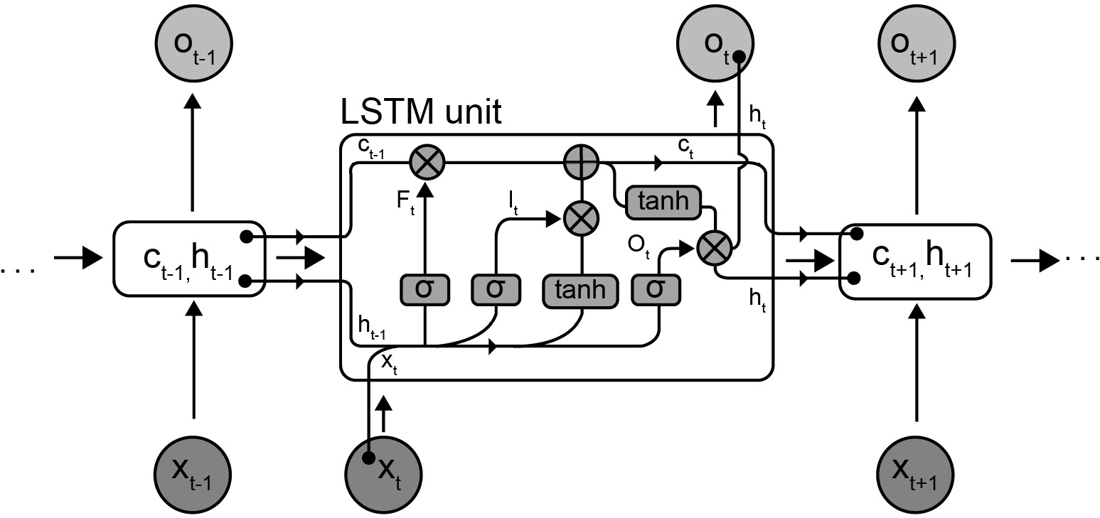
Figure 3.11: Block diagram of an LSTM

The following exercise shows how a recurrent network with LSTM units can be created using the Keras API.

Exercise 3.04: Building a Recurrent Neural Network Model with the Keras High-Level API

In this exercise, we will create a recurrent neural network using the Keras high-level API. It will have the following architecture: the very first layer is simply a layer that encodes, using certain rules, the input features, thereby producing a given set of embeddings. The second layer is a layer where 64 LSTM units are added to it. They are added inside a bidirectional wrapper, which is a specific layer that's used to improve and speed up learning by doubling the units it acts on and training the first ones with the input as-is, and the second ones with the input reversed (for example, words in a sentence read from right to left). Then, the outputs are concatenated. This technique has been proven to generate faster and better learning. Finally, two dense layers are added that have 64 and 1 neurons, respectively. Perform the following steps to complete this exercise:

1. Import the TensorFlow module and print its version:

   from __future__ import absolute_import, division,

   print_function, unicode_literals

   import tensorflow as tf

   print("TensorFlow version: {}".format(tf.__version__))

   This outputs the following line:

   TensorFlow version: 2.1.0

2. Build the model using the Keras sequential method and print the network summary:

   EMBEDDING_SIZE = 8000

   model = tf.keras.Sequential([

           tf.keras.layers.Embedding(EMBEDDING_SIZE, 64),

           tf.keras.layers.Bidirectional(tf.keras.layers.LSTM(64)),

           tf.keras.layers.Dense(64, activation='relu'),

           tf.keras.layers.Dense(1)])

   model.summary()

   In the preceding code, the model is simply built by stacking up consecutive layers. First, there is the embedding layer, then the bidirectional one, which operates on the LSTM layer, and finally two dense layers at the end of the model.

   The model summary will be as follows:

   Model: "sequential"

   _________________________________________________________________

   Layer (type) Output Shape Param #

   =================================================================

   embedding (Embedding) (None, None, 64) 512000

   _________________________________________________________________

   bidirectional (Bidirectional (None, 128) 66048

   _________________________________________________________________

   dense (Dense) (None, 64) 8256

   _________________________________________________________________

   dense_1 (Dense) (None, 1) 65

   =================================================================

   Total params: 586,369

   Trainable params: 586,369

   Non-trainable params: 0

   _________________________________________________________________

   Note

   To access the source code for this specific section, please refer to https://packt.live/3cX01OO.

   You can also run this example online at https://packt.live/37nw1ud.

With this overview of how to implement a neural network using TensorFlow, the following sections will show you how to combine all these notions to tackle typical machine learning problems, including regression and classification problems.

Simple Regression Using TensorFlow

This section will explain, step by step, how to successfully tackle a regression problem. You will learn how to take a preliminary look at the dataset to understand its most important properties, as well as how to prepare it to be used during training, validation, and inference. Then, a deep neural network will be built from a clean sheet using TensorFlow via the Keras API. This model will then be trained and its performance will be evaluated.

In a regression problem, the aim is to predict the output of a continuous value, such as a price or a probability. In this exercise, the classic Auto MPG dataset will be used and a deep neural network will be trained on it to accurately predict car fuel efficiency, using no more than the following seven features: Cylinders, Displacement, Horsepower, Weight, Acceleration, Model Year, and Origin.

The dataset can be thought of as a table with eight columns (seven features, plus one target value) and as many rows as instances the dataset has. As per the best practices we looked at in the previous sections, it will be divided as follows: 20% of the total number of instances will create the test set, while the remaining ones will be split again into training and validation sets with an 80:20 ratio.

As a first step, the training set will be inspected for missing values, and cleaned if needed. Then, a chart showing variable correlation will be plotted. The only categorical variable present will be converted into numerical form via one-hot encoding. Finally, all the features will be normalized.

The deep learning model will then be created. A three-layered fully connected architecture will be used: the first and the second layer will have 64 nodes, while the last one, being the output layer of a regression problem, will have only one node.

Standard choices for the loss function (mean squared error) and optimizer (RMSprop) will be applied. Training will then be performed with and without early stopping to highlight the different effects they have on training and validation loss.

Finally, the model will be applied to the test set to evaluate performances and make predictions.

Exercise 3.05: Creating a Deep Neural Network to Predict the Fuel Efficiency of Cars

In this exercise, we will build, train, and measure performances of a deep neural network model that predicts car fuel efficiency using only seven car features: Cylinders, Displacement, Horsepower, Weight, Acceleration, Model Year, and Origin.

The step-by-step procedure for this is as follows:

1. Import all the required modules and print the versions of the most important ones:

   from __future__ import absolute_import, division,

   print_function, unicode_literals

   import matplotlib.pyplot as plt

   import numpy as np

   import pandas as pd

   import seaborn as sns

   import tensorflow as tf

   print("TensorFlow version: {}".format(tf.__version__))

   The output will be as follows:

   TensorFlow version: 2.1.0

2. Import the Auto MPG dataset, read it with pandas, and show the last five rows:

   dataset_path = tf.keras.utils.get_file("auto-mpg.data",

                  "https://raw.githubusercontent.com/"

                  "PacktWorkshops/"

                  "The-Reinforcement-Learning-Workshop/master/"

                  "Chapter03/Dataset/auto-mpg.data")

   column_names = ['MPG','Cylinders','Displacement','Horsepower',

                   'Weight', 'Acceleration', 'Model Year', 'Origin']

   raw_dataset = pd.read_csv(dataset_path, names=column_names,

                             na_values = "?", comment=' ',

                             sep=" ", skipinitialspace=True)

   dataset = raw_dataset.copy()

   dataset.tail()

   Note

   Watch out for the slashes in the string below. Remember that the backslashes ( ) are used to split the code across multiple lines, while the forward slashes ( / ) are part of the URL.

   The output will be as follows:

   

   Figure 3.12: Last five rows of the dataset imported in pandas

3. Let's clean the data from unknown values. Check how much Not available data is present and where:

   dataset.isna().sum()

   This produces the following output:

   MPG 0

   Cylinders 0

   Displacement 0

   Horsepower 6

   Weight 0

   Acceleration 0

   Model Year 0

   Origin 0

   dtype: int64

4. Given the small number of rows with unknown values, simply drop them:

   dataset = dataset.dropna()

5. Use one-hot encoding for the Origin variable, which is categorical:

   dataset['Origin'] = dataset['Origin']

                       .map({1: 'USA', 2: 'Europe', 3: 'Japan'})

   dataset = pd.get_dummies(dataset, prefix='', prefix_sep='')

   dataset.tail()

   The output will be as follows:

   

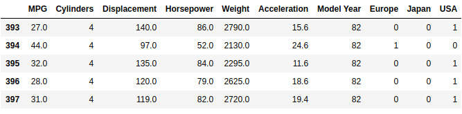
   Figure 3.13: Last five rows of the dataset imported into pandas using one-hot encoding

6. Split the data into training and test sets with an 80:20 ratio:

   train_dataset = dataset.sample(frac=0.8,random_state=0)

   test_dataset = dataset.drop(train_dataset.index)

7. Now, let's take a look at some training data statistics, that is, the joint distributions of some pairs of features from the training set, using the seaborn module. The pairplot command takes in the features of the dataset as input to evaluate them, couple by couple. Along the diagonal (where the couple is composed of two instances of the same feature), it shows the distribution of the variable, while in the off-diagonal terms, it shows the scatterplot of the two features. This is useful if we wish to highlight correlations:

   sns.pairplot(train_dataset[["MPG", "Cylinders", "Displacement",

                               "Weight"]], diag_kind="kde")

   This generates the following image:

   

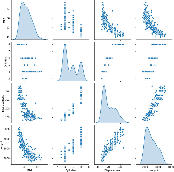
   Figure 3.14: Joint distributions of some pairs of features from the training set

8. Let's now take a look at the overall statistics:

   train_stats = train_dataset.describe()

   train_stats.pop("MPG")

   train_stats = train_stats.transpose()

   train_stats

   The output will be as follows:

   

   Figure 3.15: Overall training set statistics

9. Split the features from the labels and normalize the data:

   train_labels = train_dataset.pop('MPG')

   test_labels = test_dataset.pop('MPG')

   def norm(x):

       return (x - train_stats['mean']) / train_stats['std']

   normed_train_data = norm(train_dataset)

   normed_test_data = norm(test_dataset)

10. Now, let's look at the model's creation and a summary of the same:

    def build_model():

        model = tf.keras.Sequential([

                tf.keras.layers.Dense(64, activation='relu',

                                      input_shape=[len

                                      (train_dataset.keys())]),

                tf.keras.layers.Dense(64, activation='relu'),

                tf.keras.layers.Dense(1)])

        optimizer = tf.keras.optimizers.RMSprop(0.001)

        model.compile(loss='mse', optimizer=optimizer,

                      metrics=['mae', 'mse'])

        return model

    model = build_model()

    model.summary()

    This generates the following output:

    

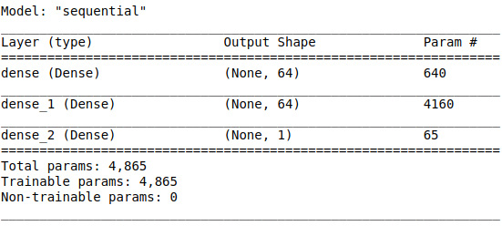
    Figure 3.16: Model summary

11. Use the fit model function to train the network for 1,000 epochs by using a validation set of 20%:

    epochs = 1000

    history = model.fit(normed_train_data, train_labels,

                        epochs=epochs, validation_split = 0.2,

                        verbose=2)

    This will produce a very long output. We will only report the last few lines here:

    Epoch 999/1000251/251 - 0s - loss: 2.8630 - mae: 1.0763

    - mse: 2.8630 - val_loss: 10.2443 - val_mae: 2.3926

    - val_mse: 10.2443

    Epoch 1000/1000251/251 - 0s - loss: 2.7697 - mae: 0.9985

    - mse: 2.7697 - val_loss: 9.9689 - val_mae: 2.3709 - val_mse: 9.9689

12. Visualize the training and validation metrics by plotting the MAE and MSE.

    The following snippet plots the MAE:

    hist = pd.DataFrame(history.history)

    hist['epoch'] = history.epoch

    plt.plot(hist['epoch'],hist['mae'])

    plt.plot(hist['epoch'],hist['val_mae'])

    plt.ylim([0, 10])

    plt.ylabel('MAE [MPG]')

    plt.legend(["Training", "Validation"])

    The output will be as follows:

    

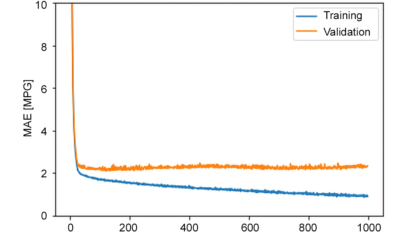
    Figure 3.17: Mean absolute error over the plot of epochs

    The preceding figure shows how increasing the training epochs causes the validation error to grow, meaning the system is experiencing an overfitting problem.

13. Now, let's visualize the MSE using a plot:

    plt.plot(hist['epoch'],hist['mse'])

    plt.plot(hist['epoch'],hist['val_mse'])

    plt.ylim([0, 20])

    plt.ylabel('MSE [MPG^2]')

    plt.legend(["Training", "Validation"])

    The output will be as follows:

    

    Figure 3.18: Mean squared error over the plot of epochs

    Also, in this case, the figure shows how increasing the training epochs causes the validation error to grow, meaning the system is experiencing an overfitting problem.

14. Use Keras callbacks to add early stopping (with the patience parameter equal to 10 epochs) to avoid overfitting. First of all, build the model:

    model = build_model()

15. Then, define an early stopping callback. This entity will be passed to the model.fit function and will be called every fit step to check whether the validation error stops decreasing for more than 10 consecutive epochs:

    early_stop = tf.keras.callbacks

                 .EarlyStopping(monitor='val_loss', patience=10)

16. Finally, call the fit method with the early stop callback:

    early_history = model.fit(normed_train_data, train_labels,

                              epochs=epochs, validation_split=0.2,

                              verbose=2, callbacks=[early_stop])

    The last few lines of the output are as follows:

    Epoch 42/1000251/251 - 0s - loss: 7.1298 - mae: 1.9014

    - mse: 7.1298 - val_loss: 8.1151 - val_mae: 2.1885

    - val_mse: 8.1151

    Epoch 43/1000251/251 - 0s - loss: 7.0575 - mae: 1.8513

    - mse: 7.0575 - val_loss: 8.4124 - val_mae: 2.2669

    - val_mse: 8.4124

17. Visualize the train and validation metrics for early stopping. Firstly, collect all the training history data and put it into a pandas DataFrame, for both the metric and epoch values:

    early_hist = pd.DataFrame(early_history.history)

    early_hist['epoch'] = early_history.epoch

18. Then, plot the training and validation MAE against the epochs, limiting the max y values to 10:

    plt.plot(early_hist['epoch'],early_hist['mae'])

    plt.plot(early_hist['epoch'],early_hist['val_mae'])

    plt.ylim([0, 10])

    plt.ylabel('MAE [MPG]')

    plt.legend(["Training", "Validation"])

    The preceding code will produce the following output:

    

    Figure 3.19: Mean absolute error over the plot of epochs (early stopping)

    As demonstrated by the preceding figure, training is stopped as soon as the validation error stops decreasing, thereby avoiding overfitting.

19. Evaluate the model accuracy on the test set:

    loss, mae, mse = model.evaluate(normed_test_data,

                                    test_labels, verbose=2)

    print("Testing set Mean Abs Error: {:5.2f} MPG".format(mae))

    The output will be as follows:

    78/78 - 0s - loss: 6.3067 - mae: 1.8750 - mse: 6.3067

    Testing set Mean Abs Error: 1.87 MPG

    Note

    The accuracy may show slightly different values due to random sampling with a variable random seed.

20. Finally, perform model inference by predicting all the MPG values for all test instances. Then, plot these values with respect to their true values so that you have a visual estimation of the model error:

    test_predictions = model.predict(normed_test_data).flatten()

    a = plt.axes(aspect='equal')

    plt.scatter(test_labels, test_predictions)

    plt.xlabel('True Values [MPG]')

    plt.ylabel('Predictions [MPG]')

    lims = [0, 50]

    plt.xlim(lims)

    plt.ylim(lims)

    _ = plt.plot(lims, lims)

    The output will be as follows:

    

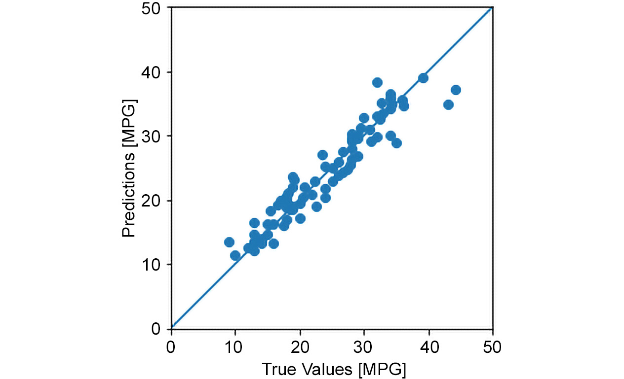
Figure 3.20: Predictions versus ground truth scatterplot

The scatterplot puts predicted values versus true values in correspondence with one another, which means that the closer the points are to the diagonal line, the more accurate the predictions will be. It is evident how clustered the points are, meaning predictions are fairly accurate.

Note

To access the source code for this specific section, please refer to https://packt.live/3feCLNN.

You can also run this example online at https://packt.live/37n5WeM.

This section has shown how to successfully tackle a regression problem. The selected dataset has been imported, cleaned, and subdivided into training, validation, and test sets. Then, a brief exploratory data analysis was carried out before a three-layered fully connected deep neural network was created. The network has been successfully trained and its performance has been evaluated on the test set.

Now, let's study classification problems using TensorFlow.

Simple Classification Using TensorFlow

This section will help you understand and solve a typical supervised learning problem that falls under the category conventionally named classification.

Classification tasks, in their simplest generic form, aim to associate one category, among a predefined set, with instances. An intuitive example of a classification task that's often used for introductory courses is classifying the images of domestic pets in the correct category they belong to, such as "cat" or "dog." Classification plays a fundamental role in many everyday activities and can easily be encountered in different contexts. The previous example is a specific case of classification called image classification, and many similar applications can be found in this category.

However, classification extends beyond images. The following are some examples:

• Customer classification for video recommendation systems (answering the question, "In which market segment this user falls?")
• Spam filters ("What are the chances this email is spam?")
• Malware detection ("Is this program a cyber threat?")
• Medical diagnosis ("Is this patient sick?")

For image classification tasks, images are fed to the classification algorithm as inputs, and it returns the class they belong to as output. Images are three-dimensional arrays of numbers representing per-pixel brightness (height x width x number of channels, where color images have three channels – red, green, blue (RGB) – and grayscale images only have one), and these numbers are the features that the algorithm uses to determine the class images belong to.

When dealing with other types of inputs, features can be different. For example, in the case of a medical diagnosis classification system, blood test parameters, age, sex, and suchlike can be features that are used by the algorithm to identify the class the instance belongs to, that is, "sick" or "not sick."

In the following exercise, we will create a deep neural network by building upon what we described in the previous sections. This will be able to achieve an accuracy of around 70% when classifying signals that have been detected inside a simulated ATLAS experiment, distinguishing between background noise and Higgs Boson Tau-Tau decay using a set of 28 features: yes, machine learning applied to particle physics!

Note

For additional information on the dataset, visit the official website: http://archive.ics.uci.edu/ml/datasets/HIGGS.

Given the huge size of the dataset, to keep the exercise easy to run and still meaningful, it will be subsampled: 10,000 rows will be used for training and 1,000 rows each for validation and test. Three different models will be trained: a small model that will be a reference (two layers with 16 and 1 neurons each), a large model with no overfit countermeasures (five layers; four with 512 neurons and the last one with 1 neuron) to demonstrate problems that may be encountered in this scenario, and then regularization and dropout will be added to the large model, effectively limiting overfitting and improving performance.

Exercise 3.06: Creating a Deep Neural Network to Classify Events Generated by the ATLAS Experiment in the Quest for Higgs Boson

In this exercise, we will build, train, and measure the performance of a deep neural network in order to improve the discovery significance of the ATLAS experiment by using simulated data with features for characterizing events. The task is to classify events into two categories: "tau decay of a Higgs Boson" versus "background."

This dataset can be found in the TensorFlow dataset (https://www.tensorflow.org/datasets), which is a collection of ready-to-use datasets. It is available to download and interface via the processing pipeline. In our case, the original dataset is too big for our purposes, so we will postpone dataset usage until we get to this chapter's activity. For now, we will use a subgroup of the dataset that's directly available through the repository.

Note

You can find the dataset in this book's GitHub repository here: https://packt.live/3dUfYq8.

The step-by-step procedure is described in detail as follows:

1. Import all the required modules and print the versions of the most important ones:

   from __future__ import absolute_import, division,

   print_function, unicode_literals

   from IPython import display

   from matplotlib import pyplot as plt

   from scipy.ndimage.filters import gaussian_filter1d

   import pandas as pd

   import numpy as np

   import tensorflow as tf

   print("TensorFlow version: {}".format(tf.__version__))

   The output will be as follows:

   TensorFlow version: 2.1.0

2. Import the dataset and prepare the data for preprocessing.

   For this exercise, we will download a custom-made smaller subset that's been pulled from the original dataset:

   higgs_path = tf.keras.utils.get_file('HIGGSSmall.csv.gz',

                'https://github.com/PacktWorkshops/'

                'The-Reinforcement-Learning-Workshop/blob/'

                'master/Chapter03/Dataset/HIGGSSmall.csv.gz?raw=true')

3. Read the CSV dataset into a TensorFlow dataset class and repack it so that it has tuples (features, labels):

   N_TEST = int(1e3)

   N_VALIDATION = int(1e3)

   N_TRAIN = int(1e4)

   BUFFER_SIZE = int(N_TRAIN)

   BATCH_SIZE = 500

   STEPS_PER_EPOCH = N_TRAIN//BATCH_SIZE

   N_FEATURES = 28

   ds = tf.data.experimental

        .CsvDataset(higgs_path,[float(),]*(N_FEATURES+1),

                    compression_type="GZIP")

   def pack_row(*row):

       label = row[0]

       features = tf.stack(row[1:],1)

       return features, label

   packed_ds = ds.batch(N_TRAIN).map(pack_row).unbatch()

   Take a look at the value distribution of the features:

   for features,label in packed_ds.batch(1000).take(1):

       print(features[0])

       plt.hist(features.numpy().flatten(), bins = 101)

   The output will be as follows:

   tf.Tensor(

   [ 0.8692932 -0.6350818 0.22569026 0.32747006 -0.6899932

   0.7542022 -0.2485731 -1.0920639 0. 1.3749921

   -0.6536742 0.9303491 1.1074361 1.1389043 -1.5781983

   -1.0469854 0. 0.65792954 -0.01045457 -0.04576717

   3.1019614 1.35376 0.9795631 0.97807616 0.92000484

   0.72165745 0.98875093 0.87667835], shape=(28,), dtype=float32)

   The plot will be as follows:

   

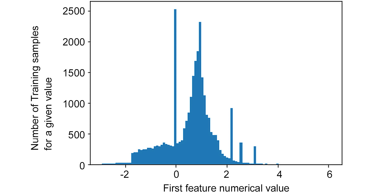
   Figure 3.21: First feature value distribution

   In the preceding graph, the x axis represents the number of training samples for a given value, while the y axis denotes the first feature's numerical value.

4. Create training, validation, and test sets:

   validate_ds = packed_ds.take(N_VALIDATION).cache()

   test_ds = packed_ds.skip(N_VALIDATION).take(N_TEST).cache()

   train_ds = packed_ds.skip(N_VALIDATION+N_TEST)

              .take(N_TRAIN).cache()

5. Define feature, label, and class names:

   feature_names = ["lepton pT", "lepton eta", "lepton phi",

                    "missing energy magnitude",

                    "missing energy phi",

                    "jet 1 pt", "jet 1 eta", "jet 1 phi",

                    "jet 1 b-tag",

                    "jet 2 pt", "jet 2 eta", "jet 2 phi",

                    "jet 2 b-tag",

                    "jet 3 pt", "jet 3 eta", "jet 3 phi",

                    "jet 3 b-tag",

                    "jet 4 pt", "jet 4 eta", "jet 4 phi",

                    "jet 4 b-tag",

                    "m_jj", "m_jjj", "m_lv", "m_jlv", "m_bb",

                    "m_wbb", "m_wwbb"]

   label_name = ['Measure']

   class_names = ['Signal', 'Background']

   print("Features: {}".format(feature_names))

   print("Label: {}".format(label_name))

   print("Class names: {}".format(class_names))

   The output will be as follows:

   Features: ['lepton pT', 'lepton eta', 'lepton phi',

   'missing energy magnitude', 'missing energy phi',

   'jet 1 pt', 'jet 1 eta', 'jet 1 phi', 'jet 1 b-tag',

   'jet 2 pt', 'jet 2 eta', 'jet 2 phi', 'jet 2 b-tag',

   'jet 3 pt', 'jet 3 eta', 'jet 3 phi', 'jet 3 b-tag',

   'jet 4 pt', 'jet 4 eta', 'jet 4 phi', 'jet 4 b-tag',

   'm_jj', 'm_jjj', 'm_lv', 'm_jlv', 'm_bb', 'm_wbb', 'm_wwbb']

   Label: ['Measure']

   Class names: ['Signal', 'Background']

6. Show a sample of a training instance for features and labels:

   features, labels = next(iter(train_ds))

   print("Features =")

   print(features.numpy())

   print("Labels =")

   print(labels.numpy())

   The output will be as follows:

   Features =

   [ 0.3923715 1.3781117 1.5673449 0.17123567 1.6574531

   0.86394763 0.88821083 1.4797885 2.1730762 1.2008675

   0.9490923 -0.30092147 2.2148721 1.277294 0.4025028

   0.50748837 0. 0.50555664

   -0.55428815 -0.7055601 0. 0.94152564 0.9448251

   0.9839765 0.7801499 1.4989641 0.91668195 0.8027126 ]

   Labels = 0.0

7. Assign a batch size to the datasets:

   test_ds = test_ds.batch(BATCH_SIZE)

   validate_ds = validate_ds.batch(BATCH_SIZE)

   train_ds = train_ds.shuffle(BUFFER_SIZE).repeat()

              .batch(BATCH_SIZE)

8. Now, let's start creating the model and training it. Create a decaying learning rate:

   lr_schedule = tf.keras.optimizers.schedules

                 .InverseTimeDecay(0.001,

                                   decay_steps=STEPS_PER_EPOCH*1000,

                                   decay_rate=1, staircase=False)

9. Define a function that will compile a model with an Adam optimizer, use binary cross entropy as the loss function, and fit it on training data by using early stopping on the validation dataset.

   The function takes in the model as input, chooses the Adam optimizer, and compiles the model with it, as well as with the binary cross entropy loss and the accuracy metrics:

   def compile_and_fit(model, name, max_epochs=3000):

       optimizer = tf.keras.optimizers.Adam(lr_schedule)

       model.compile(optimizer=optimizer,

       loss=tf.keras.losses.BinaryCrossentropy(from_logits=True),

       metrics=[tf.keras.losses.BinaryCrossentropy(from_logits=True,

                name='binary_crossentropy'),'accuracy'])

   A summary of the model is then printed, as follows:

       model.summary()

10. The model is then fitted on the training dataset using a validation dataset and the early stopping callback. The training history is saved and returned as output:

        history = model.fit(train_ds,

                  steps_per_epoch = STEPS_PER_EPOCH,

                  epochs=max_epochs, validation_data=validate_ds,

                  callbacks=[tf.keras.callbacks

                             .EarlyStopping

                             (monitor='val_binary_crossentropy',

                             patience=200)],verbose=2)

        return history

11. Create a small model with just two layers with 16 and 1 neurons, respectively, and compile it and fit it on the dataset:

    small_model = tf.keras.Sequential([

                  tf.keras.layers.Dense(16, activation='elu',

                                        input_shape=(N_FEATURES,)),

                  tf.keras.layers.Dense(1)])

    size_histories = {}

    size_histories['small'] = compile_and_fit(small_model, 'sizes/small')

    This will produce a long output, where the last two lines will be similar to the following:

    Epoch 1522/3000

    20/20 - 0s - loss: 0.5693 - binary_crossentropy: 0.5693

    - accuracy: 0.6846 - val_loss: 0.5841

    - val_binary_crossentropy: 0.5841 - val_accuracy: 0.6640

    Epoch 1523/3000

    20/20 - 0s - loss: 0.5695 - binary_crossentropy: 0.5695

    - accuracy: 0.6822 - val_loss: 0.5845

    - val_binary_crossentropy: 0.5845 - val_accuracy: 0.6600

12. Check the model's performance on the test set:

    test_accuracy = tf.keras.metrics.Accuracy()

    for (features, labels) in test_ds:

        logits = small_model(features)

        probabilities = tf.keras.activations.sigmoid(logits)

        predictions = 1*(probabilities.numpy() > 0.5)

        test_accuracy(predictions, labels)

        small_model_accuracy = test_accuracy.result()

    print("Test set accuracy:{:.3%}".format(test_accuracy.result()))

    The output will be as follows:

    Test set accuracy: 68.200%

    Note

    The accuracy may show slightly different values due to random sampling with a variable random seed.

13. Create a large model with five layers – four with 512 neurons and the last one with 1 neuron, respectively – and compile and fit it:

    large_model = tf.keras.Sequential([

                  tf.keras.layers.Dense(512, activation='elu',

                                        input_shape=(N_FEATURES,)),

                  tf.keras.layers.Dense(512, activation='elu'),

                  tf.keras.layers.Dense(512, activation='elu'),

                  tf.keras.layers.Dense(512, activation='elu'),

                  tf.keras.layers.Dense(1)])

    size_histories['large'] = compile_and_fit(large_model, "sizes/large")

    This will produce a long output, where the last two lines will be similar to the following:

    Epoch 221/3000

    20/20 - 0s - loss: 1.0285e-04 - binary_crossentropy: 1.0285e-04

    - accuracy: 1.0000 - val_loss: 2.5506

    - val_binary_crossentropy: 2.5506 - val_accuracy: 0.6660

    Epoch 222/3000

    20/20 - 0s - loss: 1.0099e-04 - binary_crossentropy: 1.0099e-04

    - accuracy: 1.0000 - val_loss: 2.5586

    - val_binary_crossentropy: 2.5586 - val_accuracy: 0.6650

14. Check the model's performance on the test set:

    test_accuracy = tf.keras.metrics.Accuracy()

    for (features, labels) in test_ds:

        logits = large_model(features)

        probabilities = tf.keras.activations.sigmoid(logits)

        predictions = 1*(probabilities.numpy() > 0.5)

        test_accuracy(predictions, labels)

        large_model_accuracy = test_accuracy.result()

        regularization_model_accuracy = test_accuracy.result()

    print("Test set accuracy: {:.3%}"

          . format(regularization_model_accuracy))

    The output will be as follows:

    Test set accuracy: 65.200%

    Note

    The accuracy may show slightly different values due to random sampling with a variable random seed.

15. Create the same large model as before, but add regularization items such as L2 regularization and dropout. Then, compile it and fit the model to the set:

    regularization_model = tf.keras.Sequential([

                           tf.keras.layers.Dense(512,

                           kernel_regularizer=tf.keras.regularizers

                                              .l2(0.0001),

                           activation='elu',

                           input_shape=(N_FEATURES,)),

                           tf.keras.layers.Dropout(0.5),

                           tf.keras.layers.Dense(512,

                           kernel_regularizer=tf.keras.regularizers

                                              .l2(0.0001),

                           activation='elu'),

                           tf.keras.layers.Dropout(0.5),

                           tf.keras.layers.Dense(512,

                           kernel_regularizer=tf.keras.regularizers

                                              .l2(0.0001),

                           activation='elu'),

                           tf.keras.layers.Dropout(0.5),

                           tf.keras.layers.Dense(512,

                           kernel_regularizer=tf.keras.regularizers

                                              .l2(0.0001),

                           activation='elu'),

                           tf.keras.layers.Dropout(0.5),

                           tf.keras.layers.Dense(1)])

    size_histories['regularization'] = compile_and_fit

                                       (regularization_model,

                                        "regularizers/regularization",

                                        max_epochs=9000)

    This will produce a long output, where the last two lines will be similar to the following:

    Epoch 1264/9000

    20/20 - 0s - loss: 0.5873 - binary_crossentropy: 0.5469

    - accuracy: 0.6978 - val_loss: 0.5819

    - val_binary_crossentropy: 0.5416 - val_accuracy: 0.7030

    Epoch 1265/9000

    20/20 - 0s - loss: 0.5868 - binary_crossentropy: 0.5465

    - accuracy: 0.7024 - val_loss: 0.5759

    - val_binary_crossentropy: 0.5356 - val_accuracy: 0.7100

16. Check the model's performance on the test set:

    test_accuracy = tf.keras.metrics.Accuracy()

    for (features, labels) in test_ds:

        logits = regularization_model (features)

        probabilities = tf.keras.activations.sigmoid(logits)

        predictions = 1*(probabilities.numpy() > 0.5)

        test_accuracy(predictions, labels)

    print("Test set accuracy: {:.3%}".format(test_accuracy.result()))

    The output will be as follows:

    Test set accuracy: 69.300%

    Note

    The accuracy may show slightly different values due to random sampling with a variable random seed.

17. Compare the binary cross entropy trend of the three models over epochs:

    histSmall = pd.DataFrame(size_histories["small"].history)

    histSmall['epoch'] = size_histories["small"].epoch

    histLarge = pd.DataFrame(size_histories["large"].history)

    histLarge['epoch'] = size_histories["large"].epoch

    histReg = pd.DataFrame(size_histories["regularization"].history)

    histReg['epoch'] = size_histories["regularization"].epoch

    trainSmoothSmall = gaussian_filter1d

                       (histSmall['binary_crossentropy'], sigma=3)

    testSmoothSmall = gaussian_filter1d

                      (histSmall['val_binary_crossentropy'], sigma=3)

    trainSmoothLarge = gaussian_filter1d

                       (histLarge['binary_crossentropy'], sigma=3)

    testSmoothLarge = gaussian_filter1d

                      (histLarge['val_binary_crossentropy'], sigma=3)

    trainSmoothReg = gaussian_filter1d

                     (histReg['binary_crossentropy'], sigma=3)

    testSmoothReg = gaussian_filter1d

                    (histReg['val_binary_crossentropy'], sigma=3)

    plt.plot(histSmall['epoch'], trainSmoothSmall, '-',

             histSmall['epoch'], testSmoothSmall, '--')

    plt.plot(histLarge['epoch'], trainSmoothLarge, '-',

             histLarge['epoch'], testSmoothLarge, '--')

    plt.plot(histReg['epoch'], trainSmoothReg, '-',

             histReg['epoch'], testSmoothReg, '--',)

    plt.ylim([0.5, 0.7])

    plt.ylabel('Binary Crossentropy')

    plt.legend(["Small Training", "Small Validation",

                "Large Training", "Large Validation",

                "Regularization Training",

                "Regularization Validation"])

    This will produce the following graph:

    

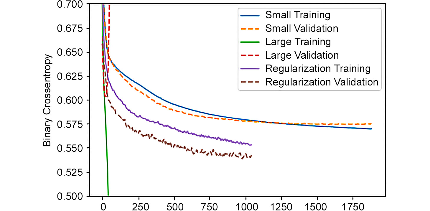
    Figure 3.22: Binary cross entropy comparison

    The preceding graph shows a comparison of the different models, in terms of both training and validation errors, to demonstrate how overfitting works. The training error goes down for each of them as the number of training epochs increases. The validation error for the large model, on the other hand, rapidly increases after a certain number of epochs. In the small model, it goes down, following the training error closely and reaching a final performance that is worse than the one obtained by the model with regularization, which avoids overfitting and has the best performance among the three.

18. Compare the accuracy trend of the three models over epochs:

    trainSmoothSmall = gaussian_filter1d

                       (histSmall['accuracy'], sigma=6)

    testSmoothSmall = gaussian_filter1d

                      (histSmall['val_accuracy'], sigma=6)

    trainSmoothLarge = gaussian_filter1d

                       (histLarge['accuracy'], sigma=6)

    testSmoothLarge = gaussian_filter1d

                      (histLarge['val_accuracy'], sigma=6)

    trainSmoothReg = gaussian_filter1d

                     (histReg['accuracy'], sigma=6)

    testSmoothReg = gaussian_filter1d

                    (histReg['val_accuracy'], sigma=6)

    plt.plot(histSmall['epoch'], trainSmoothSmall, '-',

             histSmall['epoch'], testSmoothSmall, '--')

    plt.plot(histLarge['epoch'], trainSmoothLarge, '-',

             histLarge['epoch'], testSmoothLarge, '--')

    plt.plot(histReg['epoch'], trainSmoothReg, '-',

             histReg['epoch'], testSmoothReg, '--',)

    plt.ylim([0.5, 0.75])

    plt.ylabel('Accuracy')

    plt.legend(["Small Training", "Small Validation",

                "Large Training", "Large Validation",

                "Regularization Training",

                "Regularization Validation",])

    This will produce the following graph:

    

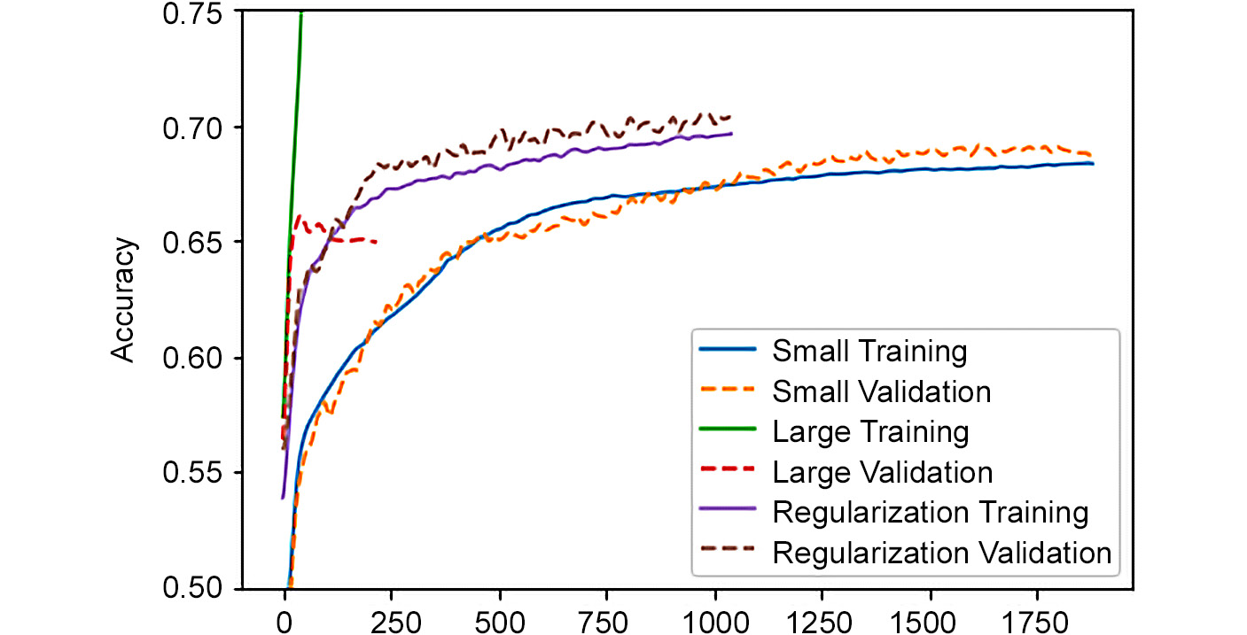
Figure 3.23: Accuracy comparison

In a specular way with respect to the previous one, this graph shows, once again, a comparison of the different models, but in terms of accuracy. The training accuracy grows for each model when the number of training epochs increases. The validation accuracy for the large model, on the other hand, stops growing after a certain number of epochs. In the small model, it goes up, following the training one closely and reaching a final performance that is worse than the one obtained by the model with regularization, which avoids overfitting and attains the best performance among the three.

Note

To access the source code for this specific section, please refer to https://packt.live/37m9huu.

You can also run this example online at https://packt.live/3hhIDaZ.

In this section, we solved a fancy classification problem, resulting in the creation of a deep learning model able to achieve about 70% accuracy when classifying Higgs boson-related signals using simulated ATLAS experiment data. After a first general overview of the dataset, where we understood how it is arranged and the nature of its features and labels, a set of three deep fully connected neural networks were created using the Keras API. These models were trained and tested, and their performances in terms of loss and accuracy over epochs have been compared, thereby giving us a firm grasp of the overfitting problem and which techniques help in solving it.

TensorBoard – How to Visualize Data Using TensorBoard

TensorBoard is a web-based tool embedded in TensorFlow. It provides a suite of methods that we can use to get insights into TensorFlow sessions and graphs, thus allowing the user to inspect, visualize, and understand them deeply. It provides access to many functionalities in a straightforward way, as follows:

• It allows us to explore the details of TensorFlow model graphs, making the user able to zoom in to specific blocks and subsections.
• It can generate plots of typical quantities of interest that we can take a look at during training, such as loss and accuracy.
• It gives us access to histogram visualizations that show tensors changing over time.
• It provides trends of layer weights and bias over epochs.
• It stores runtime metadata for a run, such as total memory usage.
• It visualizes embeddings.

TensorBoard reads TensorFlow log files containing summary information about the training process at hand. These are generated with the appropriate callbacks, which are then passed to TensorFlow jobs.

The following screenshot shows some typical visualizations that are provided by TensorBoard. The first one is the "Scalars" section, which shows scalar quantities associated with the training stage. In this example, accuracy and binary cross entropy are being represented:

Figure 3.24: TensorBoard scalars

The second view provides a block diagram visualization of the computational graph, where all the layers are reported together with their relations, as shown in the following screenshot:

Figure 3.25: TensorBoard graph

The DISTRIBUTIONS tab provides an overview of how the model parameters are distributed across epochs, as shown in the following figure:

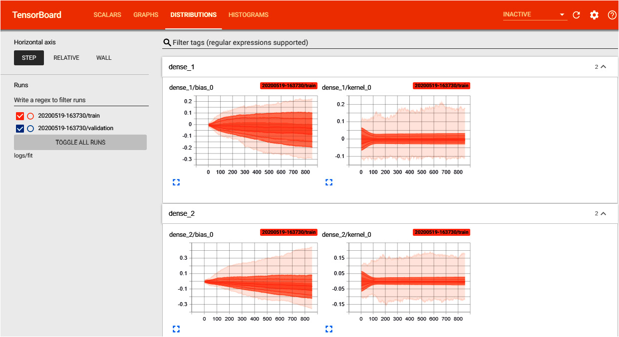
Figure 3.26: TensorBoard distributions

Finally, the HISTOGRAMS tab provides similar information to the DISTRIBUTIONS tab, but is unfolded in 3D, as shown in the following screenshot:

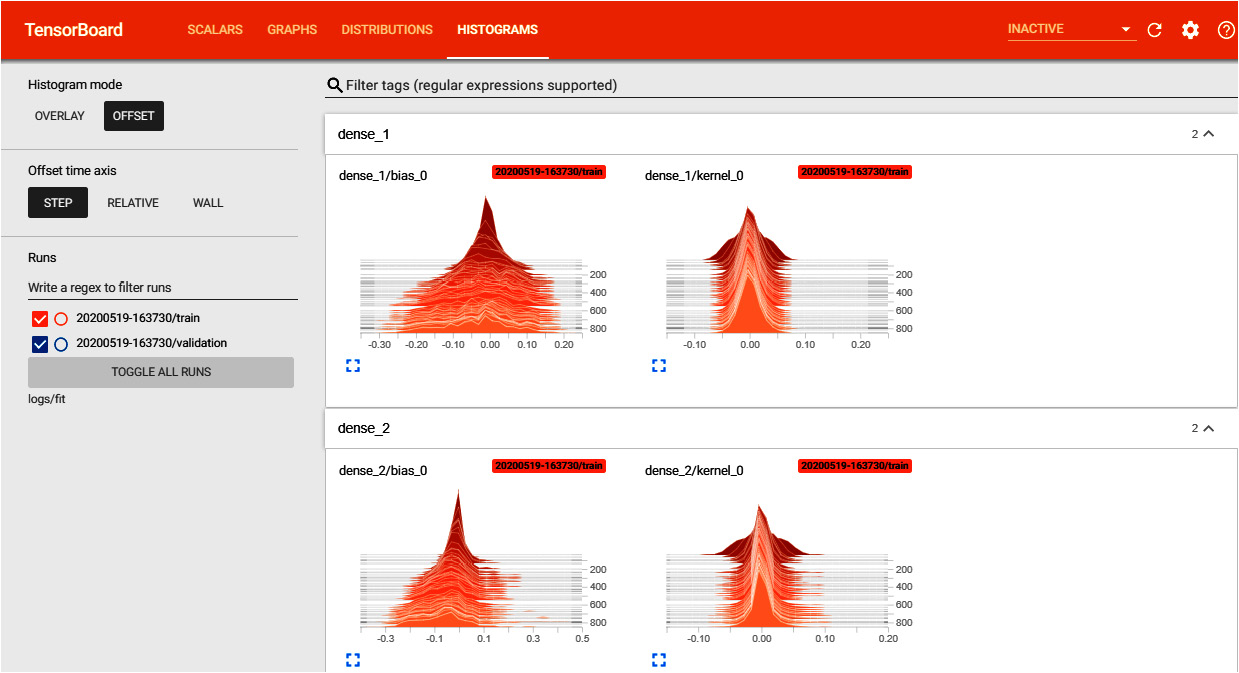
Figure 3.27: TensorBoard histograms

In this section and, in particular, in the following exercise, TensorBoard will be leveraged to easily visualize metrics in terms of trends, tensor graphs, distributions, and histograms.

In order to focus only on TensorBoard, the very same classification exercise we performed in the previous section will be used. Only the large model will be trained. All we need is to import TensorBoard and activate it, as well as a definition of the log file directory.

A TensorBoard callback is then created and passed to the fit method of the model. This will generate all TensorBoard files inside the log directory. Once training is complete, this log directory path is passed to TensorBoard as an argument. This will open a web-based visualization where the user is able to gain deep insights into its model and training-related aspects.

Exercise 3.07: Creating a Deep Neural Network to Classify Events Generated by the ATLAS Experiment in the Quest for the Higgs Boson Using TensorBoard for Visualization

In this exercise, we will build, train, and measure the performance of a deep neural network with the same goal of Exercise 3.06, Creating a Deep Neural Network to Classify Events Generated by the ATLAS Experiment in the Quest for Higgs Boson in mind, but instead, we will leverage TensorBoard so that we can gain additional training insights.

The following steps need to be implemented in order to complete this exercise:

1. Import all the required modules:

   from __future__ import absolute_import, division,

   print_function, unicode_literals

   from IPython import display

   from matplotlib import pyplot as plt

   from scipy.ndimage.filters import gaussian_filter1d

   import pandas as pd

   import numpy as np

   import datetime

   import tensorflow as tf

   !rm -rf ./logs/

   # Load the TensorBoard notebook extension

   %load_ext tensorboard

2. Download the custom smaller subset of the original dataset:

   higgs_path = tf.keras.utils.get_file('HIGGSSmall.csv.gz',

                'https://github.com/PacktWorkshops/'

                'The-Reinforcement-Learning-Workshop/blob/master/'

                'Chapter03/Dataset/HIGGSSmall.csv.gz?raw=true')

3. Read the CSV dataset into the TensorFlow dataset class and repack it so that it has tuples (features, labels):

   N_TEST = int(1e3)

   N_VALIDATION = int(1e3)

   N_TRAIN = int(1e4)

   BUFFER_SIZE = int(N_TRAIN)

   BATCH_SIZE = 500

   STEPS_PER_EPOCH = N_TRAIN//BATCH_SIZE

   N_FEATURES = 28

   ds = tf.data.experimental.CsvDataset

        (higgs_path,[float(),]*(N_FEATURES+1),

         compression_type="GZIP")

   def pack_row(*row):

       label = row[0]

       features = tf.stack(row[1:],1)

       return features, label

   packed_ds = ds.batch(N_TRAIN).map(pack_row).unbatch()

4. Create training, validation, and test sets and assign them the BATCH_SIZE parameter:

   validate_ds = packed_ds.take(N_VALIDATION).cache()

   test_ds = packed_ds.skip(N_VALIDATION).take(N_TEST).cache()

   train_ds = packed_ds.skip(N_VALIDATION+N_TEST)

              .take(N_TRAIN).cache()

   test_ds = test_ds.batch(BATCH_SIZE)

   validate_ds = validate_ds.batch(BATCH_SIZE)

   train_ds = train_ds.shuffle(BUFFER_SIZE)

              .repeat().batch(BATCH_SIZE)

5. Now, let's start creating the model and training it. Create a decaying learning rate:

   lr_schedule = tf.keras.optimizers.schedules

                 .InverseTimeDecay(0.001,

                                   decay_steps=STEPS_PER_EPOCH*1000,

                                   decay_rate=1, staircase=False)

6. Define a function that will compile a model with the Adam optimizer and use binary cross entropy as the loss function. Then, fit it on the training data using early stopping by using the validation dataset, as well as a TensorBoard callback:

   log_dir = "logs/fit/" + datetime.datetime.now()

             .strftime("%Y%m%d-%H%M%S")

   def compile_and_fit(model, name, max_epochs=3000):

       optimizer = tf.keras.optimizers.Adam(lr_schedule)

       model.compile(optimizer=optimizer,

       loss=tf.keras.losses.BinaryCrossentropy(from_logits=True),

       metrics=[tf.keras.losses.BinaryCrossentropy

               (from_logits=True, name='binary_crossentropy'),

                'accuracy'])

       model.summary()

       tensorboard_callback = tf.keras.callbacks.TensorBoard

                              (log_dir=log_dir,

                               histogram_freq=1,

                               profile_batch=0)

       history = model.fit

                 (train_ds,

                  steps_per_epoch = STEPS_PER_EPOCH,

                  epochs=max_epochs,

                  validation_data=validate_ds,

                  callbacks=[tf.keras.callbacks.EarlyStopping

                            (monitor='val_binary_crossentropy',

                             patience=200),

                             tensorboard_callback],               verbose=2)

       return history

7. Create the same large model as before with regularization items such as L2 regularization and dropout, and then compile it and fit it on the dataset:

   regularization_model = tf.keras.Sequential([

                          tf.keras.layers.Dense(512,

                          kernel_regularizer=tf.keras.regularizers

                                             .l2(0.0001),

                          activation='elu',

                          input_shape=(N_FEATURES,)),

                          tf.keras.layers.Dropout(0.5),

                          tf.keras.layers.Dense(512,

                          kernel_regularizer=tf.keras.regularizers

                                             .l2(0.0001),

                          activation='elu'),

                          tf.keras.layers.Dropout(0.5),

                          tf.keras.layers.Dense(512,

                          kernel_regularizer=tf.keras.regularizers

                                             .l2(0.0001),

                          activation='elu'),

                          tf.keras.layers.Dropout(0.5),

                          tf.keras.layers.Dense(512,

                          kernel_regularizer=tf.keras.regularizers

                                             .l2(0.0001),

                          activation='elu'),

                          tf.keras.layers.Dropout(0.5),

                          tf.keras.layers.Dense(1)])

   compile_and_fit(regularization_model,

                   "regularizers/regularization", max_epochs=9000)

   The last output line will be as follows:

   Epoch 1112/9000

   20/20 - 1s - loss: 0.5887 - binary_crossentropy: 0.5515

   - accuracy: 0.6949 - val_loss: 0.5831

   - val_binary_crossentropy: 0.5459 - val_accuracy: 0.6960

8. Check the model's performances on the test set:

   test_accuracy = tf.keras.metrics.Accuracy()

   for (features, labels) in test_ds:

       logits = regularization_model(features)

       probabilities = tf.keras.activations.sigmoid(logits)

       predictions = 1*(probabilities.numpy() > 0.5)

       test_accuracy(predictions, labels)

   print("Test set accuracy: {:.3%}".format(test_accuracy.result()))

   The output will be as follows:

   Test set accuracy: 69.300%

   Note

   The accuracy may show slightly different values due to random sampling with a variable random seed.

9. Visualize the variables with TensorBoard:

   %tensorboard --logdir logs/fit

   This command starts the web-based visualization tool. Four main windows are represented in the following figure, displaying information about loss and accuracy, model graphs, histograms, and distributions in a clockwise order, starting from the top left:

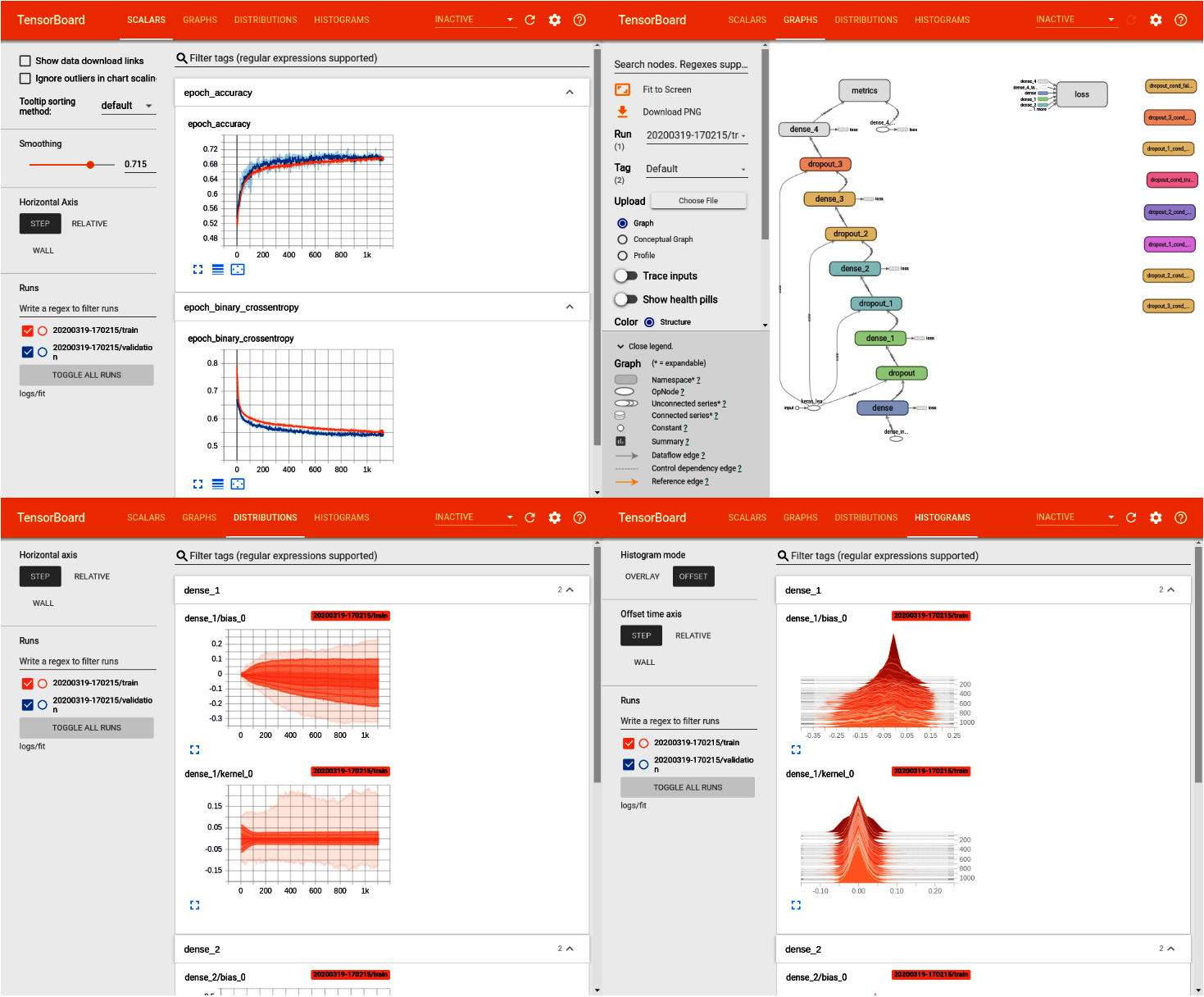
Figure 3.28: TensorBoard visualization

The advantages of using TensorBoard are quite evident: all the training information is collected in a single place, allowing the user to easily navigate through it. The top-left panel, the SCALARS tab, allows the user to monitor loss and accuracy so that they are able to check the same chart we saw previously in an easier way.

In the top right, the model graph is shown, so it is possible to visualize how input data flows into the computational graph by going through each block.

The two views at the bottom show the same information in two different representations: all the model parameter (networks weights and biases) distributions are shown across training epochs. On the left, the DISTRIBUTIONS tab displays the parameters in 2D, while the HISTOGRAMS tab unfolds the parameters in 3D. They both allow the user to monitor how trainable parameters vary during the training step.

Note

To access the source code for this specific section, please refer to https://packt.live/2AWGjFv.

You can also run this example online at https://packt.live/2YrWl2d.

In this section, we focused on providing some insights into how to use TensorBoard to visualize training-related model parameters. We saw how, starting with an already familiar problem, it is super easy to add the TensorBoard web-based visualization tool and navigate through all of its plugins directly inside a Python notebook.

Now, let's complete an activity to put all our knowledge to the test.

Activity 3.01: Classifying Fashion Clothes Using a TensorFlow Dataset and TensorFlow 2

Suppose you need to code an image processing algorithm for a company that owns a clothes warehouse. They want to autonomously classify clothes based on a camera output, thereby allowing them to group clothes together with no human intervention.

In this activity, we will create a deep fully connected neural network capable of doing such a task, meaning that it will accurately classify images of clothes by assigning them to the class they belong to.

The following steps will help you to complete this activity:

1. Import all the required modules, such as numpy, matplotlib.pyplot, tensorflow, and tensorflow_datasets, and print out their main module versions.
2. Import the Fashion MNIST dataset using TensorFlow datasets and split it into train and test sets.
3. Explore the dataset to get familiar with the input features, that is, shapes, labels, and classes.
4. Visualize some instances of the training set.
5. Perform data normalization by building the classification model.
6. Train the deep neural network.
7. Test the model's accuracy. You should obtain an accuracy in excess of 88%.
8. Perform inference and check the predictions against the ground truth.

   By the end of this activity, the trained model should be able to classify all the fashion items (clothes, shoes, bags, and so on) with an accuracy greater than 88%, thus producing a result similar to the one shown in the following image:

Figure 3.29: Clothes classification with a deep neural network output

Note

The solution to this activity can be found on page 696.

Summary

In this chapter, we were introduced to practical deep learning with TensorFlow 2 and Keras, their key features and applications, and how they work together. We became familiar with the differences between low- and high-level APIs, as well as how to leverage the most advanced modules to ease the creation of deep models. Then, we discussed how to implement a deep neural network with TensorFlow and addressed some major topics: from model creation, training, validation, and testing, we highlighted the most important aspects to consider so as to avoid pitfalls. We saw how to build different types of deep learning models, such as fully connected, convolutional, and recurrent neural networks, via the Keras API. We solved a regression task and a classification problem, which gave us hands-on experience with this. We learned how to leverage TensorBoard to visualize many different training trends regarding metrics and model parameters. Finally, we built and trained a model that is able to classify fashion item images with high accuracy, an activity that shows that a possible real-world problem can be solved with the help of the most advanced deep learning techniques.

In the next chapter, we will be studying the OpenAI Gym environment and how to use TensorFlow 2 for reinforcement learning.