Chapter 5
The Long and the Short of It
Our analysis in Chapter 4 suggested that the implied volatility skew tends to be mispriced in the sense that there is excess demand for moderately out-of-the-money options. But what of the term structure? We want to say something about the value embedded in near-term options compared with longer-dated ones. Here, it is more difficult to be precise. Judging from broker flows, it seems as though institutional managers favour hedges with a few months to maturity. It is uncommon to see strategies that rely upon rolling weekly options and strategies that incorporate multi-year options (outside of the interest rate markets) seem equally rare. We can start with the hypothesis that, if there is any value to be found along the term structure, it probably resides with options that have a very long or very short time to maturity. We want to avoid medium-term options. If everyone wants to buy something, it's going to be expensive.
SHORT-DATED OPTIONS
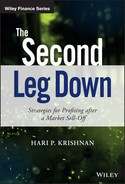
Some traders argue that you don't want to hold options that are close to expiration. The standard argument is that short-dated options have the highest time decay. Figure 5.1 calculates the time decay of ATM options on the S&P 500 as a function of time to maturity. So if you buy a fixed dollar amount of options with different maturities and nothing happens on a given day, the short-dated ones will lose the most. This is true for any delta, e.g. a fixed dollar amount of short-dated 25 delta puts decay more rapidly than a fixed amount of longer-dated 25 delta puts. However, when you buy short-dated protection after a volatility spike, a number of things work in your favour. We explore these in the next section.
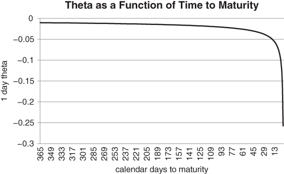
Figure 5.1 Time decay for a fixed delta option accelerates as maturity is approached
One way to study options is to analyse the extreme cases in time (maturity) and space (strike). For example, you can gain insights by comparing very short-dated options with very long-dated ones. Very short-dated options are characterised by a pitched battle between gamma and theta. Every day that passes quietly will destroy a large percentage of premium. This is bad for the holder of an option. However, large moves can provide a tremendous bang for the buck. It is not unusual to make 10 or more times premium paid on a weekly option. The old venture capital “four bagger”, where you make four times your original investment, pales in comparison to what can be made here. IPO-style returns are possible, without the attendant risk.
Let's start by looking at theta, which can be misinterpreted for very short-dated options. Figure 5.1 shows the relationship between theta and time to maturity for an at-the-money option.
We have represented the data along an x-axis which is decreasing in time to maturity. This makes the severe decline in theta easier to visualise, as it occurs away from the x-axis. Since theta approaches −∞ as T − t goes to 0, it's tempting to conclude that short-dated options decay too quickly to be useful. If the underlying asset doesn't move pronto, a short-dated put will burn off. In this context, it seems as though you need to time the entry point perfectly. However, the problem can be considered from another angle. While short-dated options do have severe time decay, we would argue that they have already decayed, based on the cumulative impact of many moderately negative theta days. Their absolute prices are low, relative to the amount of coverage they can provide. Given a fixed dollar budget, you can buy a relatively large number of short-dated options. Your protection might not last too long, but in a highly volatile market can make the difference between survival and oblivion. The ability to buy large quantities of options dramatically increases your profit potential if your view is immediately validated by the market. In Figure 5.2, we follow the price decline of an ATM put as time passes, assuming no change in the spot price or volatility. The cost of putting a 1-week floor on your portfolio is roughly 1/8 that of a 1-year floor.
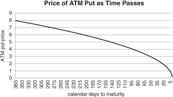
Figure 5.2 At-the-money protection rapidly cheapens near maturity
OTM puts whose strike is a fixed percentage below the spot decay even more rapidly as a percentage of premium paid. The “Batman” trade in Figure 3.27 relies upon this phenomenon. You are a net payer of premium when you buy an ATM straddle and sell 2 OTM strangles. However, your theta is still positive until close to maturity, as time decay hits the wings harder than the centre.
Short-dated puts have lots of gamma as the spot approaches the strike. By contrast, long-dated options have a much straighter profile, implying that frequent delta-hedging in response to price changes is not all that necessary. Long-dated options are far more sensitive to investor risk aversion levels than to actual changes in the price of the underlying asset. This is particularly true for low-delta options with a long time to maturity. Here, risk aversion is the code word for implied volatility. You can't hedge vega risk unless you already know what investor sentiment is going to be in the future. It might be argued that a somewhat out-of-the-money put with a day to go doesn't have much gamma, either. Strictly speaking, this is correct. The subtlety is that an OTM 1-day put has a great deal of potential gamma. Big changes in delta are not far away. A modest decline in the spot can cause the put to slingshot up the payout curve, as the option delta rapidly approaches −1. This is one of the reasons we favour weekly options as an emergency hedge. The practical issue is whether the spot can move far enough to capture the slingshot effect? We need to get a statistical handle on this question to justify a weekly options buying strategy. Ideally, we would like to see lots of unexpectedly large moves over short horizons.
For equity indices, at least, things seem to work in our favour. A relatively large number of moderate initial drops transform themselves into vicious sell-offs over horizons of a few days. Significantly, their frequency is more than a normal distribution would predict. Prices move according to a positive feedback loop, where investors are forced into the market after an initial move. Day traders and other thinly capitalised investors have to push the escape button if they are severely caught on the wrong side of a trade. Whether explicit stop orders have been placed in the market or not, one large sell order can trigger another, in sequence. Standard econometric techniques are not necessarily the right way to analyse these moves, especially if the feedback function is non-linear. Markets can move almost discontinuously from one level to another if the level of panic becomes high enough.
In the next section, we will discuss some of the statistical evidence suggesting that markets have particularly fat-tailed distributions over short horizons. For now, suppose this empirical statement is true. It follows that you can buy gamma relatively cheaply in the form of weekly options, hedging your portfolio over a horizon where the most damage can potentially be done. If you buy and hold medium maturity options, you will have effectively paid premium over a horizon where market returns tend to be relatively benign. This reduces the expected return of an OTM hedge.
THE PHYSICISTS WEIGH IN
Numerous physicists and applied mathematicians have tried their hand at analysing financial data over the years.These were the early “big data” scientists, as financial markets had an abundance of data and few solid theoretical underpinnings. Over 50 years ago, Mandelbrot (1963) theorised that fluctuations in financial market prices might have infinite variance. Here was a man well ahead of his time, at least in this respect. The true volatility of a stock might be infinite.
Digest that for a moment. A distribution with infinite volatility (or variance) is a far cry from a normal distribution, whose every moment is finite. Moves in excess of 5 or 6 standard deviations essentially never occur for a normal distribution. The tails decay rapidly enough that the expectation of returns, returns squared, returns cubed and so on are all well-defined. Mandelbrot observed explosion in the second moment when analysing historical cotton prices. If correct, the main consequence of the random walk hypothesis would be invalidated. Asset price returns would not be remotely normal. Over time, the weaker notion that asset returns are non-normal has become widely accepted. The question is to what degree extreme events are underpriced by the random walk hypothesis. Conventional academics have a tendency to “stretch” standard models in an attempt to explain outlying data. They might add intermittent jumps to a Gaussian distribution, but are reluctant to develop entirely new models to account for outsized moves.
Are normal distributions accurate, first-order approximations of financial reality, or are they wildly inaccurate in times of crisis? Infinite variance suggests wild inaccuracy, but there are situations where returns look at least relatively normal. As we will soon see, one answer to this question depends on the investment time horizon. Many years later, Taleb (2007) managed to shoehorn Mandelbrot's ideas into a barbell approach to asset allocation. On the assumption that extreme events are statistically underpriced (both in terms of frequency and impact), he advocated a portfolio of safe short-term government bonds combined with a sprinkling of high risk speculative bets where you could lose no more than your initial investment. This is a radical departure from traditional portfolio theory, on the assumption that long-term returns may have greater dependence on the tails than the centre of the distribution.
We tip our hat to Taleb, but have more modest objectives. Our goal is to summarise some of the research suggesting that stock indices have fat-tailed distributions over short horizons.This research has practical application to weekly options. To our knowledge, the relevance of results from econophysics to weekly options has never received much attention and we believe that the discussion below is novel. The application of techniques from statistical physics and dynamical systems to large quantities of financial data is sometimes called “econophysics”. This melding of disciplines gained traction about 20 years ago. Previously, financial economists had never been particularly focused on high-frequency data in their ongoing search for risk premia, which can only be extracted over long horizons. Yet masses of intraday data had been available for many years and by the 1990s, computers were powerful enough to process the data. Here, we restrict ourselves to a summary of a paper written by Stanley's group at Boston University in the late 1990s, namely Gopikrishnan (1999). Incidentally, it appears as though it was Stanley himself who coined the term “econophysics” (as in Gangopadhyay, 2013), so we are certainly going to the source. Our overriding goal is to demonstrate that low delta weekly options may be statistically cheap. The paper tracks the quantities P(ξ > X) and P(ξ < − X), as X gets large. These define the “asymptotics” or extremes of a distribution. Note that P(ξ >X) is the probability that a random draw ξ from the underlying distribution is greater than the threshold X. P(ξ >X) says something about the right tail of the distribution and P(ξ < −X) about the left tail. We focus on the left tail here, as it refers to downside risk for stock indices and other risky assets. These are the sorts of things we typically need to hedge. If returns were normally distributed, P(ξ < − X) would decay faster than 1/X(α) for any α, as X goes to infinity. But this does not turn out to be the case over short-term horizons. Over 1-minute intervals, the authors find that the left-tail alpha is roughly equal to 3. In other words, the tail decays at a rate proportional to 1/X3. This suggests that the distribution is not normal, but may satisfy a power law at the extremes. The variance of large moves is probably finite, but skewness and higher moments are likely to be infinite. We can't say with certainty that the variance of 1-minute returns is finite because of the “Mexican peso problem”: the mega standard deviation event may simply not have been observed yet.
As the partition window extends beyond a day, we revert to daily data over a 35-year horizon. Alpha slowly increases as a function of window size, suggesting gradual convergence to a normal distribution. Extrapolating from the data, 1-day 10 standard deviation returns are expected to occur once every 10,000 trading days or so. By contrast, a 1 in 10,000 downside move is expected to be roughly 4 standard deviations in magnitude with a partition width of 16 days. This pales in magnitude to what we see in the data.
Gopikrishnan (1999) argues that the mechanism for fat tails over short horizons is serial correlation. Big moves have a tendency to pile up in the same direction. For the S&P 500, we observe that the autocorrelation of returns increases as the partition width contracts toward 0. Persistence is the mechanism that creates fat tails in the distribution over short horizons. Selling can beget more selling, as short-term traders chase the move and others are forced into the market in an attempt to manage their risk. This implies that we can use weekly options reactively. If there is a significant down move, we can bet on continuation using a short-dated put, with the statistical evidence in our favour. We don't need to roll our weekly options mechanically every week, as that would be prohibitively expensive. Rather, we can wait for the market to tumble, on the assumption that the probability of an extreme left-tail event over the next few days has increased. If history is a guide, you will usually get some warning before the market breaks through. A weekly options strategy can be implemented more cheaply and sparingly using a reactive approach. We conclude with a few words of caution. While many futures contracts trade overnight, weekly options contracts generally do not. This implies that you can't protect against weekend or overnight events using a weekly options strategy. You need to wait until the cash open to activate a hedge. This suggests that weekly options need to be supplemented with a less timing-dependent hedging strategy. The other obstacle is liquidity. While S&P 500, Euro Stoxx 50 and selected individual stock and ETF weeklies are relatively liquid, the range of tradable weekly options is still quite small. If you need to hedge an idiosyncratic or esoteric risk falling outside of this domain, you may be out of luck.
The following lines from the abstract are particularly significant:
We can see that there is a fairly sharp transition from heavy-tailed to nearly Gaussian behaviour at the 4-day mark. This implies that we would be well-served to focus on options with 4 days or less to go, namely weekly options after the weekend has passed. Intra-week options give us exposure over time horizons where the underlying distribution has the heaviest tails. It's a happy coincidence that the tails are fattest over horizons where vega is lowest. If the market attempts to adjust for increased forward risk by bidding up implied volatility, we can simply move to a further OTM strike to reduce our vega exposure.
While weekly options are an appealing way to react to short-term drops, they are not foolproof. Naturally, this is true of every options strategy. If markets sell off into a Friday close, there is not much we can do. We lose our theoretical edge if we buy a put expiring on the next Friday, as the option has 7 days to go. The underlying distribution is likely to be relatively Gaussian over this horizon. If we adhere strictly to the results of the paper, maintaining continuous coverage through a rolling weekly options strategy is going to be expensive.
A rolling strategy with weekly puts of a given delta generally requires greater premium outlay than one using monthly puts. If we fix the delta at 25, say, the weekly put strikes will start much closer to the spot than the monthly ones. This is a nice feature, but refreshing the strike each week comes at a cost. In Figure 5.3, we make the rough assumption that a month is exactly 4 weeks long. We then compare the price of 41-week 25 delta puts to 11-month 25 delta put for the Euro Stoxx 50 index. We have departed from the S&P 500 in this example purely for the sake of variety.
Figure 5.3 Mechanically refreshing weekly puts can be expensive
Buying and re-loading weekly options usually requires between 2 and 2.5 times as much premium as the equivalent monthly put strategy. Viewed from the standpoint of rolling costs, weekly options are egregiously expensive. This serves as an admonition that you should only buy weekly options when you need them. You can only go to the well so many times before the cost of hedging becomes prohibitive. The market is declaring that the “refresh” option for weekly puts has significant value. Weeklies will wind up in the money far more frequently than monthlies.
The reader may have observed that our analysis is heavily dependent on research that is nearly 20 years old. What if things have changed since then? Without replicating the study completely, we now give circumstantial evidence that scaling laws for price fluctuations haven't changed materially over time. We start our analysis with S&P 500 index futures. First, we calculate the standard deviation σ (21) of 21-day returns, using data from 1995 to 2015. This period roughly picks up where the Stanley group study left off. Note that there are roughly 21 trading days in a calendar month, so this is a reasonable convention. We then convert σ to a standard deviation for each series of n day returns. ![]() would be the correct transformation for all n, assuming that prices evolved according to a random walk. In our example, n ranges from 1 to 25 days. What is the meaning of this transformation? In the world of Brownian motion, where the standard deviation of returns fans out at a rate equal to
would be the correct transformation for all n, assuming that prices evolved according to a random walk. In our example, n ranges from 1 to 25 days. What is the meaning of this transformation? In the world of Brownian motion, where the standard deviation of returns fans out at a rate equal to ![]() , we would expect the percentage of returns greater than
, we would expect the percentage of returns greater than ![]() to be independent of n. In particular, the frequency of “2 sigma” events should be roughly 4.55% for any partition n. Recall that, when you sample from a normal distribution, 95.45% of all samples are expected to lie within 2 standard deviations of the mean. Equivalently, 4.55% of all samples are expected to be 2+ standard deviation events. The random walk construction does not turn out to be correct, as Figure 5.4 suggests.
to be independent of n. In particular, the frequency of “2 sigma” events should be roughly 4.55% for any partition n. Recall that, when you sample from a normal distribution, 95.45% of all samples are expected to lie within 2 standard deviations of the mean. Equivalently, 4.55% of all samples are expected to be 2+ standard deviation events. The random walk construction does not turn out to be correct, as Figure 5.4 suggests.
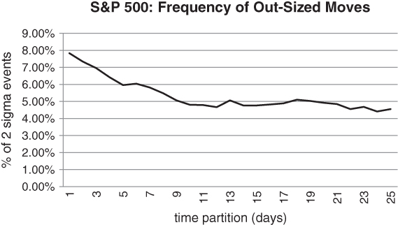
Figure 5.4 Frequency of 2+ standard deviation returns in S&P 500, based on partition width
For 1-day returns, the incidence of 2+ standard deviation returns is nearly twice what σ (21) would predict. There are lots of outliers over horizons less than a week. As the partition width grows, the extremes of our distribution look increasingly normal. The curve settles down to the 4.5% target level as we move to the right of Figure 5.4. This suggests that, after a large short-term drop, the index has a tendency to mean revert. At the very least, it doesn't tend to follow through. Note that we haven't considered long partition widths (i.e. where n is large), as we would then have to take the average return of the series into account. We would then be calculating deviations from an average historical return that may be quite different in the future.
We now branch out into other equity indices, as in the Stanley group paper. In Figure 5.5, we can see that the FTSE 100 and DAX indices follow roughly the same descending path. Figure 5.5 takes a simple average of the FTSE and DAX curves, for each partition width. In technical terms, we have calculated a rough version of the Hurst exponent, as in Beran (1994). This measures the range over which a stochastic process has “memory”.
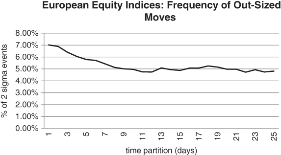
Figure 5.5 Frequency of 2+ standard deviation returns, DAX/FTSE blend
We can move even further afield, without much difficulty. Figure 5.6 tabulates the frequency of 2+ standard deviation moves for a concentrated global portfolio of bond futures. In particular, we have taken an equally weighted combination of US 10 year, Bund and JGB (Japanese Government Bond) futures. As above, we have averaged the frequencies across the 3 contracts, using data from 1995 to 2015.
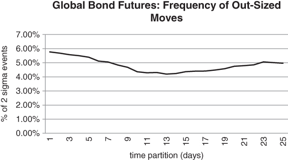
Figure 5.6 Frequency of 2+ standard deviation returns in global bond futures markets
Now we are faced with a more complicated situation. We observe the usual decay from 1- to roughly 10-day partitions. However, the curve now turns up for wider partition widths. This gives us the impression of an asset class where there are big intra-week returns that stall a bit and then follow through. This may be a momentum effect. Bonds have a greater tendency to trend over medium- to long-horizons, exaggerating an initial sharp short-term move. In Chapter 6, we will describe how bond futures have been very “trend worthy” since the 1980s. For now, we observe one other stylised fact. The bond futures curve never seems to wander too far from the 4.55% theoretical level. In this sense, bonds are more well-behaved than equity indices over short horizons. Having said that, it may be that the infrequent 2 standard deviation moves are much larger than a normal distribution would predict.
We end this section with an ideological point. If you use options to hedge or express a view, you may be picking relatively low hanging fruit. Most empirical research attempts to characterise the price dynamics of “primitive” securities, such as stocks and bonds, rather than derivatives, such as options. By contrast, options research has typically focused on pricing relative to an underlying asset. Derman (2016) has succinctly compared this to calculating the fair value of a fruit salad based on the price of the constituent fruits. But there is another alternative. As an investor in options, you can study the literature on underlying asset returns and see if it has application to the options structures you trade. We have tried to follow this prescription here.
BUYING TIME
When markets are volatile and profits are draining away, many discretionary traders find their eyes glued to the screen. They start to watch every tiny move, every tick, in the markets they trade. This is an affliction without any logical basis. What can you gain from watching the ticks? If you don't know how you will react to a given market move before it occurs, tracking the market offers no advantage. In a thought-provoking article, Gray (2014) argues that algorithms can outperform human judgment in many fields where it is tacitly assumed that experts should have superior insight. You might make bad decisions in the heat of battle if you haven't planned ahead. Systematic funds might argue that model-based trading eliminates the need for screen watching. Systems are not robots who think for themselves. Rather, they rely upon rules developed and tested by humans, far from the market frenzy. When a grandmaster is defeated by a computer, the implication that the computer is “smarter” than the player is false. The computer is simply a composite of a calculator, a database and the collaborative effort of other masters and developers in a research setting. These allow the computer to assess a given position in relatively broad terms.
In the same way, discretionary traders need time to react appropriately to market dynamics. Yet the market affords no such luxury. It keeps moving without regard for your position. So how can you buy yourself time in a market that waits for no one? Even if you are model-based, market conditions can change beyond the confines of the data over which your system was developed. Weekly options can help. They allow you to formulate an exit strategy, at low cost. Weeklies are currently available on major equity indices, stocks and ETFs in the US. Some exchanges even support “flex” options, where you can specify the strike and time to maturity that you wish to trade. So in many instances, it should be possible to construct a hedge that tides you over for a few days.
The following example highlights the potential utility of weekly options. Let's assume that a trader has bought a 1×2 put ratio spread on the S&P 500 at the worst possible time. Specifically, 100 1-year ATM puts have been bought and 200 1-year 25 delta puts sold. As soon as the combo went through the market, there was a flash −5% move in the index. 1-year volatility spiked by 5 points across all strikes (note that this simplifying assumption understates the skew effects in the trade). The structure is instantly in trouble. A range of catastrophic scenarios is now in play, as Figure 5.7 suggests.
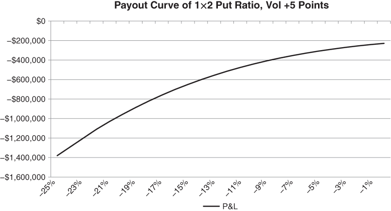
Figure 5.7 Impact of volatility expansion on a long-dated 1×2 put ratio
In all likelihood, things will calm down eventually. For the moment, however, holding on seems like a game of Russian roulette. What is the appropriate course of action now? You could just throw in the towel and liquidate the position at the close of what has been a devastating day. However, you are likely to get out at a horrible price as long-dated options are not going to be trading much. Other investors will also be scrambling to cover their short volatility positions. This will cause implied volatility to jump across all strikes and maturities. The deformable surface will rise and become more contorted. Market makers will extract their pound of flesh, given your desperation.
Another alternative is simply to pray that the markets recover overnight. This may sound absurd, but it is surprisingly common. All you need is a quick return to “rationality” from the market. When prices move against some traders, they do nothing, expecting the market to come back. No contingency is in place. Usually their positions do recover, which has a damaging psychological effect in the long-term. It reinforces reckless behaviour. Anyone who has teetered on the edge of the abyss, taken no action and been rewarded for it is likely to do the same again. Eventually, the market doesn't recover and their accounts are wiped out. After a spike in volatility, the 1×2 ratio from Figure 5.7 looks even more attractive to someone who trades mean reversion in volatility and the skew. The static “edge” in the structure has increased. The trouble is that you need the spread to converge now or else you may be forced out at an even worse level. Inexperienced traders often take aggressive short volatility positions with open-ended risk. As Ed Seykota notably said in Schwager (2012) “there are old traders and there are bold traders, but there are no old bold traders”.
The vega profile of a 1×2 put ratio illustrates how quickly you can land into trouble. We can see from Figure 5.8 that vega sharply increases in magnitude, leveling off only when the index has plunged over −15%.
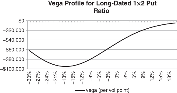
Figure 5.8 Short vega exposure for a 1×2 put ratio, as a function of moneyness
As the S&P drops, you are faced with the double whammy of increasing delta and vega. If you feel that volatility is over-priced, but need to block out the risk of an extreme downside price move, short-dated gamma hedging is appropriate. Weekly options can gear into a move faster than any algorithm, as their price responds continuously to changes in the spot. They are your ultimate defense against runaway algorithms, allowing you to focus on your core areas of expertise. The overriding conclusion is that specific options strategies can allow “old school” managers to keep investing the way they always have, while defending against runaway markets.
In Figure 5.9, we plot the payout curve for a put with 1 day to go against a put with 1 year to go. The implied volatility for both options is assumed to be constant and independent of the spot price.
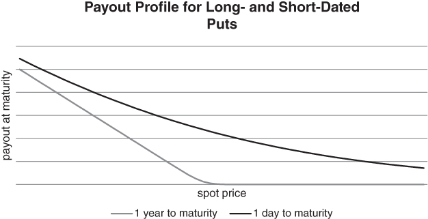
Figure 5.9 Long-dated puts have relatively high premium and vega, but relatively low gamma near the strike
We can see that OTM puts without much time to maturity trade at a low absolute price. This implies that we could buy 100 short-term puts against our 1×2 ratio spread to cap extreme event risk, while buying ourselves some time. Either the trade will recover or we can unwind some of the 1×2 while monetising some profits on the short-dated hedge.
For the 1×2 put ratio in 100 lots, your maximum exposure is roughly $20 million. If the index drops enough, you are effectively short 100 puts with delta 100. Assuming an index value of 2000 in this scenario and a multiplier of 100, your exposure is ![]() . Suppose you want to eliminate gamma risk over a 2-day horizon, using 10 delta puts. If implied volatility is 15%, these puts will cost a bit more than $1, with strike less than 2% below the spot. This implies that your 100 lot hedge will cost roughly
. Suppose you want to eliminate gamma risk over a 2-day horizon, using 10 delta puts. If implied volatility is 15%, these puts will cost a bit more than $1, with strike less than 2% below the spot. This implies that your 100 lot hedge will cost roughly ![]() , or 0.05% of notional exposure. This can be a reasonable one-off cost for a few days of sanity!
, or 0.05% of notional exposure. This can be a reasonable one-off cost for a few days of sanity!
In 2015 and 2016, there have been a few high-profile fund closures where managers argued that algorithmic trading had interfered with their core investment strategy. High-frequency mega moves were periodically occurring that seemed unrelated to what the managers considered to be market fundamentals. Anecdotally, we know that high-frequency systems typically rely on price and volume data when deciding whether to buy or sell. They're looking at information in the order book, as it evolves over time. Most systems fall into one of two categories, momentum and mean reversion. The impact of a well-capitalised mean reversion strategy is usually not much of a concern, as these strategies tend to push prices back into a range. It's momentum that we need to worry about, leading to blisteringly fast moves in one direction or another. Hammering the point home again, this is where weekly options can come in handy. Weekly options can gear into a move faster than any algorithm, as their price responds continuously to changes in the spot. You needn't worry so much about premium expansion, given the short time to maturity. They are your ultimate defence against runaway algorithms, allowing you to focus on your core areas of expertise.
LONG-DATED OPTIONS
Options with a long time to maturity, i.e. where T-t is large, have very different characteristics from short-dated ones. Gamma is relatively unimportant, as the payout curve is not very convex. At the other end of the spectrum, options with more than a year to maturity (i.e. long-dated options) can offer interesting and alternative hedging opportunities. As usual, we are trying to avoid those 2% OTM 3 month to maturity puts that many institutions seem to favour. While short-dated options tend to be gamma plays, vega plays a relatively important role when you buy a 5 year to maturity put on the S&P 500. One way to think about this is to compare the vega/theta ratio for fixed-delta options with different times to maturity.
Figure 5.10 shows the near-linear dependence of vega/theta on time to maturity. To be precise, we have calculated vega and theta for an ATM put trading at 20% implied volatility for a range of maturities. The discount rate has been assumed to be 0. In reality, theta is negative for a long call or put. We have taken its absolute value before calculating vega/theta – in reality, vega/abs(theta) – for ease of exposition.
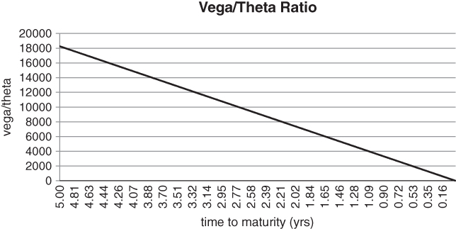
Figure 5.10 Vega/theta as a metric for selecting options
When implied volatility is low, it's logical to buy long-dated options in an effort to maximise the ratio. You can then sit back and wait for volatility to rise without worrying too much about time decay. One nice thing about long-dated implied volatility is that it isn't particularly responsive to small moves in the underlying. An uptick in the S&P 500 won't affect the value of your 2-year put in the absence of a volatility decline. Sometimes, it takes a while for a move in the underlying to propagate to the long end of the volatility term structure. The situation is a bit like a giant dinosaur that has been bitten on the tail: it might take a while before the dinosaur realises what has happened. In the early stages of a sell-off, you can sometimes buy long-dated options at implied volatility levels that have hardly moved at all. This can be very beneficial if you want to hedge without paying up for implied volatility.
There are also times when long-dated options can offer exceptional value. Structured products desks at banks occasionally create supply and demand imbalances that are not absorbed by market makers or funds that specialise in liquid exchange-traded markets. For example, when interest rates are persistently low, some banks offer yield enhancement products that rely on selling options at the long end of the curve. Japan has been in a deflationary spiral since the 1990s, with rates hovering close to 0. We mentioned how the FX carry trade has been used as a yield surrogate for Japanese investors. Option writing has also been used as an income-generating technique in Japan. At times, this has caused extreme selling pressure on long-dated puts and calls. The long end of the volatility term structure has episodically become very cheap, creating buying opportunities for value buyers of volatility.
The academic literature also provides some evidence that long-dated options might be underpriced. Pastor and Stambaugh (2012) argue against the deeply entrenched belief that annualised stock volatility is lower over longer time horizons. If the expected return of an asset is not adequately estimated by historical data, annualised volatility can actually go up as the horizon increases. This can create a rich opportunity set for buyers of long-dated options.
FAR FROM THE MADDING CROWD
Sometimes, there are isolated sell-offs in an asset class, with no immediate impact on other asset classes. For example, energies might go into a bear market, while stocks and bonds continue to rise. These episodes can offer good opportunities for long-term hedging. Ultimately, markets are linked, especially when multi-asset class investors are forced to liquidate their portfolios. If you see bad things happening in one corner of the market, a clever strategy can involve buying options elsewhere, before volatility picks up universally.
Pring (2006) has proposed the idea of an investment clock, on the assumption that asset classes move in a fairly orderly sequence. Price trends in one asset class inexorably lead to trends in the others. We start at 12 o'clock in risk off mode. Investors are piling into the safe haven of government bonds, while reducing exposure to equities and real assets. As the clock approaches 3, volatility begins to stabilise and investors start to believe that bonds have low prospective returns relative to equities. While bonds continue to rally, equities eventually enter into an upward trend. It is now 6 o'clock. Corporations are finally feeling confident enough to engage in longer-term projects. Investment capital migrates from bonds and to a lesser extent stocks into the real economy, stoking the demand for real assets. Industrial commodities such as copper and oil rally and emerging markets are starting to outperform. By 9 o'clock, inflation is ticking up to the extent that central banks want to apply the brakes. Rates begin to rise and more importantly, central banks begin to withdraw credit from the system. Bonds sell off, then equities and finally commodities. The cycle is now ready to renew itself.
We can think of sequential moves across asset classes in a less structured way. Bond investors sometimes view stock pickers with disdain, as company specialists can be the last to realise something has fundamentally changed in the economy. While they myopically scour the balance sheets of a small set of companies, the entire economy might be tumbling into recession. The bond market gives important signals that are simply ignored by the fraternity of equity analysts. Bond prices are not affected by the idiosyncratic risk in the same way that stock prices are. This implies that, in many cases, increased volatility in the bond market can be a leading indicator of equity index volatility. Assuming that the investment clock idea is correct, it has direct application to a long-dated options strategy. In the same way that broad market trends can be asynchronous, long-dated volatility does not necessary move in tandem across asset classes. There may be times where stocks are volatile but commodities are still rising, as in 2007 and early 2008. Here, you would have been well-served to buy commodity volatility as a hedge against a systemic risk event. Long-dated commodity implied volatility was still low at the end of 2007, while there had been a repricing of risk in other asset classes.
The investment management company, 36 South, has constructed a series of global implied volatility, or “GIVIX” indices, that track long-dated implied volatility across equities, FX, interest rates and commodities. The indices can be used to identify value buying opportunities in various options markets. In Figure 5.11, we can see that commodity implied volatility was slow to respond to rising equity volatility in 2007. The figure is based on the 5-year trailing Z score of the equity and commodity GIVIX indices, in an effort to normalise the two data sets.
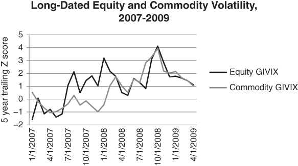
Figure 5.11 Commodity implied volatility lagged during the global financial crisis
We conclude that you can sometimes find value in long-dated options even when aggregate asset class volatility is high.
R MINUS D
Suppose we have a stock index whose price is ![]() . The risk-free rate is
. The risk-free rate is ![]() and the dividend yield of the index is
and the dividend yield of the index is ![]() . Then, a forward with time T-t to maturity will have price
. Then, a forward with time T-t to maturity will have price ![]() . The sensitivity of
. The sensitivity of ![]() to changes in
to changes in ![]() is then
is then ![]() . This is the partial derivative of
. This is the partial derivative of ![]() in
in ![]() , but we need not think in such technical terms. The key point is that, as
, but we need not think in such technical terms. The key point is that, as ![]() grows, F becomes more sensitive to
grows, F becomes more sensitive to ![]() at an exponentially increasing rate. This has major implications for options of varying maturities, as we now see.
at an exponentially increasing rate. This has major implications for options of varying maturities, as we now see.
We recall that rho (![]() ) is an option's sensitivity to small changes in interest rates. For short-dated options, rho generally isn't very important. The forward price will be quite close to the spot, regardless of rates. However, as we extend an option's time to maturity, rho plays an ever-increasing role. A small change in rates can have a relatively large impact on the price of the forward, which in turn impacts the option price. For equity indices, we need to measure sensitivity relative to
) is an option's sensitivity to small changes in interest rates. For short-dated options, rho generally isn't very important. The forward price will be quite close to the spot, regardless of rates. However, as we extend an option's time to maturity, rho plays an ever-increasing role. A small change in rates can have a relatively large impact on the price of the forward, which in turn impacts the option price. For equity indices, we need to measure sensitivity relative to ![]() , where r is the risk-free rate and d is the dividend yield of the index. If
, where r is the risk-free rate and d is the dividend yield of the index. If ![]() , the forward curve will be upward sloping, i.e. “in contango”. This implies that a 50 delta call with 1 year to maturity, say, will have a higher strike than the spot price S. In this scenario, the spot price may actually have to rally for an ATM call to wind up in the money. Suppose that we now fix r and isolate dependence on the dividend yield
, the forward curve will be upward sloping, i.e. “in contango”. This implies that a 50 delta call with 1 year to maturity, say, will have a higher strike than the spot price S. In this scenario, the spot price may actually have to rally for an ATM call to wind up in the money. Suppose that we now fix r and isolate dependence on the dividend yield ![]() .
.
The forward curve for ![]() has some interesting properties. Let's use the Euro Stoxx 50 dividend futures term structure as a guide, as dividend-based contracts have been relatively popular in France and Germany for quite some time. We observe that a futures contract is nothing more than a forward that trades on an exchange. Dividend futures trade in yearly vintages, with December expiration. For example, on 1 February, 2016, contracts ranging from December 2016 to December 2025 in annual increments were listed. The value at maturity for a given vintage is the total realised cash dividend payout for that year. Investors who rely on fundamental analysis find this feature appealing, as the terminal payout is based on genuine cash flows from companies, rather than the market's perception of what a collection of companies is worth. The futures are vectoring toward something tangible. The front-year futures are generally not that interesting, especially in the second half of the year, as most of the dividends have already been paid out. This implies that there is not much uncertainty in the payout. The front-year contract usually plods along with a volatility that converges to 0 as time goes by. However, comparing the contracts for subsequent years is instructive. In Figure 5.12, we calculate the rolling beta of the first 7 vintages to the 2nd one. Our historical data set ranges from May 2009 to January 2016.
has some interesting properties. Let's use the Euro Stoxx 50 dividend futures term structure as a guide, as dividend-based contracts have been relatively popular in France and Germany for quite some time. We observe that a futures contract is nothing more than a forward that trades on an exchange. Dividend futures trade in yearly vintages, with December expiration. For example, on 1 February, 2016, contracts ranging from December 2016 to December 2025 in annual increments were listed. The value at maturity for a given vintage is the total realised cash dividend payout for that year. Investors who rely on fundamental analysis find this feature appealing, as the terminal payout is based on genuine cash flows from companies, rather than the market's perception of what a collection of companies is worth. The futures are vectoring toward something tangible. The front-year futures are generally not that interesting, especially in the second half of the year, as most of the dividends have already been paid out. This implies that there is not much uncertainty in the payout. The front-year contract usually plods along with a volatility that converges to 0 as time goes by. However, comparing the contracts for subsequent years is instructive. In Figure 5.12, we calculate the rolling beta of the first 7 vintages to the 2nd one. Our historical data set ranges from May 2009 to January 2016.
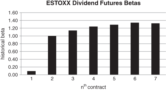
Figure 5.12 Historical beta of Euro Stoxx 50 dividend futures to 2nd contract
The 1st contract has substantially less beta than the longer-dated vintages. This is to be expected, as on average roughly 6 months of dividends have already been paid out. The uncertainty in the terminal payout is relatively low. What's more surprising is that the 2nd contract has a smaller beta than the 3rd to 7th contracts. Here, the smaller beta implies that the deferred contracts have materially higher volatility than the 2nd one. This is markedly different from what we have observed for the term structure of interest rates, volatility or commodity prices. For those markets, most of the action is in the spot and front contracts. Changes propagate through the term structure at a decaying rate. For dividend futures, conversely, a decline in corporate prospects has a disproportionate effect further down the curve. What is going on here? While dividend policy tends to be relatively fixed in the short-term, economic shocks can have a large impact on dividend policy further out into the future. A mature company will usually only cut its dividend if forced to, i.e. if it's severely strapped for cash. It's in the interest of the company to “amortise” the impact of a disastrous earnings season by gradually introducing the idea of a reduced dividend to the market. Bad news increases the probability of a slashed dividend in the somewhat distant future, after a company has prepared the market for it.
Both a call and a put are priced off the forward ![]() . If the dividend gets cut,
. If the dividend gets cut, ![]() goes up given the decline in
goes up given the decline in ![]() . This increases the value of the forward, pushing it toward the strike. An OTM call gets closer to ATM. So if you own a call on a high dividend-paying index, your existing position may actually benefit from a risk event. This may seem surprising at first, as calls are innately bullish plays. However, delta-related losses can be more than offset by rising volatility and a cut in prospective dividends. You benefit more than you might think when the dividend forward curve drops, as longer-dated options have relatively large rho (ρ). In Figure 5.13, we have calculated rho for a series of ATM puts, over a range of decreasing maturities. We have assumed that
. This increases the value of the forward, pushing it toward the strike. An OTM call gets closer to ATM. So if you own a call on a high dividend-paying index, your existing position may actually benefit from a risk event. This may seem surprising at first, as calls are innately bullish plays. However, delta-related losses can be more than offset by rising volatility and a cut in prospective dividends. You benefit more than you might think when the dividend forward curve drops, as longer-dated options have relatively large rho (ρ). In Figure 5.13, we have calculated rho for a series of ATM puts, over a range of decreasing maturities. We have assumed that ![]() is equal to 2% for all values of
is equal to 2% for all values of ![]() . We observe that the magnitude of rho decays to 0 as
. We observe that the magnitude of rho decays to 0 as ![]() approaches 0, at a roughly linear rate. Viewed differently, rho is relatively large for long-dated options.
approaches 0, at a roughly linear rate. Viewed differently, rho is relatively large for long-dated options.
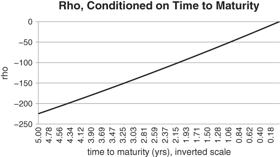
Figure 5.13 Rho has relatively large magnitude for long-dated options
Taking advantage of forward drift in a 0 interest rate environment does have some subtleties, though. The “![]() ” in
” in ![]() is nettlesome. While bank deposit rates might be 0 or even negative, the cost of borrowing the security underlying a futures contract can be quite a bit above 0. This reduces the effective drift in a long-dated call such as the one described above.
is nettlesome. While bank deposit rates might be 0 or even negative, the cost of borrowing the security underlying a futures contract can be quite a bit above 0. This reduces the effective drift in a long-dated call such as the one described above.
There are significant compensating factors. You don't have to worry too much about drift on the futures hedge, as the term structure of dividends is relatively static at the short end. Yet you are delta-neutral, long volatility and benefit from the bearish scenario where corporations start cutting their dividends. Another advantage of long-dated options can be structural. Opportunities arise now and again, as yield hogs search for a trough that generates income. In a low interest rate environment, annuity or structured note providers may try to sell long-dated puts or calls as a yield enhancer. This can artificially depress volatility at the far end of the term structure. Then, it may be possible to buy implied volatility at a discount, based on supply and demand imbalances.
Credit markets are more straightforward, in the sense that yield and the cost of hedging move in tandem. The cost of credit hedging goes up mechanically as yields increase. If you buy a high yield bond, then hedge it with a credit default swap, what you gain in yield is offset by the increased cost of default protection. For carry currencies, however, this is not necessarily the case. Suppose that an emerging market country is in a rapid growth phase. The Central Bank might raise rates in an effort to prevent the economy from overheating, i.e. to prevent inflationary bubbles. This would increase carry if you bought a forward on that country's currency. At the same time, foreign investors might be pouring money in, attracted by the country's economic prospects. So you might wind up with a situation where the spot currency was stable or rising as forward carry increased. Then, your risk-adjusted expected return would increase both as a function of higher yield and lower volatility.
If volatility goes down as carry goes up, an intriguing idea is to “spend away” a bit of excess forward yield, buying OTM puts as a direct hedge on the currency. After all, the premium on a put should be relatively low after a rally in the spot. However, there is a difficulty with this idea. While roll down pushes the forward in your favour, it reduces the effectiveness of your hedge. The forward will drift away from your put strike unless the spot currency drops sharply. The situation resembles the short VIX futures, long VIX calls hedge we analysed in Chapter 4. Roll down helps our forward, but hurts our hedge. However, as we mentioned previously, our hedge is affected by roll down at an ever-decreasing rate. Delta declines as a function of forward drift. The reader can see that many of our strategies follow the short put spread or square root (i.e. short 1×2 put ratio spread) concept. We are happy to sell nearby insurance, so long as the wings are covered or even over-hedges. The idea rhymes if not repeats. We can engage in any number of statistically based trades, so long as extreme event risk is adequately accounted for.
From a pure hedging standpoint, it would be fantastic to find a currency that had the following properties relative to a “safe” store of value such as the US dollar.
- The currency was risky, with negatively skewed returns.
- It was likely to perform poorly during a systemic risk event.
- It had a put skew that would steepen after a risk event.
- Implied volatility was currently low.
- Finally, it had a lower short rate than the equivalent maturity US T bill rate.
All the stars would be aligned. We could buy a large quantity of puts on the currency in quiet times and then wait. Our theta decay would be partially offset by downward drift in the underlying forward rate. This suggests that it would not cost much to maintain the position. In the event of a spike in global market volatility, we would benefit from increasing implied volatility and skew as well as a drop in the currency. What a nice combination! Historically, risky currencies have had relatively high interest rates, violating the final condition above. They would typically be based in emerging market or commodity producing countries, where inflation was also a concern. It is only relatively recently that currencies such as the Euro have become riskier, while engaging in competitive devaluation. As of this writing, German yields with less than 5 years to maturity are negative, offering investors cheap hedging opportunities via puts on the Euro. While it is true that the Euro put skew is already steep (loosely violating one of the conditions above), new FX hedging opportunities have emerged at a time where the 0 bound for interest rates has been breached.
THE LUMBERJACK PLOT
There is another way to visualise returns in excess of 2 standard deviations. This requires a rescaling of the axes of the cumulative distribution function. “Log log” plots are commonly used in the sciences to characterise the extremes of a distribution. The motivation is as follows. When you plot the histogram of returns for an asset, it's hard to tell how fat the tails are. The probability of an extreme event always looks very close to 0. What is needed is a technique for magnifying the tails. “Log log” graphs allow us to take an expanded view of low probability events. We can examine the left and right tails of the distribution independently, as follows. Let's start with the left tail of a standard normal distribution, i.e. a normal distribution with mean 0 and variance 1. How likely is a return smaller than −1 = −100, than −10 = −101 and so on? We can ask a sequence of questions like this and plot the result. Obviously, the sequence of probabilities decays rapidly for virtually any distribution, so we need to use a scale that accounts for very low probabilities as well. In particular, we graph the move sizes according to the sequence {−101, −102, −103, …} and the probabilities according to {−10−1, −10−2, −10−3, …} . For normal distributions, the curve decays so rapidly that you will essentially never see a move below −106, even on a scale that decays exponentially in p. Other distributions go to −∞ more slowly when plotted this way. Distributions that have fat tails may follow a “power law”, where the rate of decay is a straight line. The probability of finding a negative number that is a huge power of 10 increases proportionately as you sample 10 times as many random numbers.
We should mention that there is a region even beyond the power law. Observe that the log log graph ultimately does rely upon curve fitting. You collect lots of data, plot the probability of extreme moves on stretched axes and then fit a line through them. It may be that the regression line is so flat that the distribution appears to have infinite variance. That's already quite a statement. But what if new data points arrive that are even more extreme than the power law predicts? After all, the analysis above still relies upon extrapolation at some level. Sornette (2003) calls these outliers “dragon kings”. They are far larger than even a fitted power law distribution would predict. Assuming that we are long the tails and the dragon kings do not prevent the markets from functioning, this distinction should not concern us. When we buy enough OTM options to cover our existing positions, our potential losses are strictly bounded over the life of the options. Equivalently, we have truncated the tails of the underlying distribution. There are no tails in our composite position, so all moments in our profit and loss distribution are strictly bounded.
Vega Grows in T − t
Short-dated options have relatively little vega. Their price is not very sensitive to changes in volatility. This implies that you do not have to pay up for an OTM option after a risk event, in volatility terms. In Figure 5.14, we assume that we have taken a long position of 100 ATM puts on the S&P 500, with maturities ranging from 1 to 15 months. The term structure of volatility has been assumed constant, at 17%, across maturities. We then “shock” the term structure by +5 volatility points across all maturities and calculate the impact on the value of our puts. The long-dated options near the y-axis have considerably higher vega than the short-dated ones further to the right.
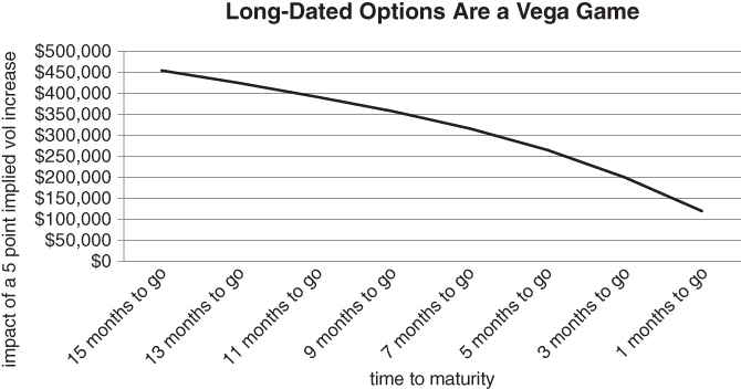
Figure 5.14 Long-dated options have relatively high sensitivity to changes in volatility
We acknowledge that the high vega in long-dated options is partially offset by the fact that long-dated volatility has a relatively low beta to short-dated volatility. It doesn't move all that much in the early phases of a sell-off. However, if there is a sustained down move, long-dated implied volatility should move enough to give you a relatively large bang for the buck.
When volatility jumps, many options become prohibitively expensive. Portfolio managers may need to hedge against disaster for a few days while they rebalance their portfolios. In this context, very short-dated options can be useful, as they are not very sensitive to changes in volatility. In this chapter, we review the literature on fat tailed distributions over short horizons. We also describe how weekly options can deliver very high payout ratios at low cost. We focus on how implied volatility can be persistent over horizons less than a week. We also discuss profit-taking strategies when delta-hedging is impossible.
SELECTIVE APPLICATION OF THE WEEKLY OPTIONS STRATEGY
In the context of crisis hedging, it's worth revisiting weekly options. We already know that the frequency of extreme moves is relatively high over intra-week horizons, but perpetually buying and rolling weeklies comes at a severe cost. However, we can selectively apply a weekly options strategy, based on the following observation. When equity markets go into a down trend, heightened risk may be in the offing. Leveraged long investors are under pressure to slash risk. It turns out that we can use a straightforward trend indicator as a buy signal for the weekly strategy. The following analysis is based on a 10-year trailing data set for the S&P 500. We have calculated the average return of a 25 delta weekly put buying strategy during up and down trends for the index. Our trend indicator simply compares the closing index value in the previous week to its trailing 52 week average. If the index is higher than the trailing average, the market is said to be in an uptrend. Otherwise, it's in a downtrend. Specifically, when the S&P was in an uptrend, the average gross return of the puts was −0.02% per week. During downtrends, which occurred less than 1/3 of the time over the sample period, the average strategy return was higher, at +0.01% per week.
Our analysis suggests that you can usually wait until the market officially goes into a downtrend before unleashing your weekly put buying strategy. Even then, you might only want to buy those puts if you really need them, in an effort to be as judicious as possible. We accept that our weekly study (i.e., using Friday close to close data) does not precisely apply to an intra-week put buying strategy. Given the results we quoted from econophysics, this may be sub-optimal. However, a fixed 1-week holding period allows us to test the relative performance of our timing strategy easily and directly.
Our trend indicator allows us to cut hedging costs by reducing the number of times we buy the weekly. In particular, we only buy after the market has given us some confirmation. This suggests that we will typically be loading the strategy after sell-off, when volatility is relatively high. It's worth confirming that the relative cost of the weekly put strategy is not too sensitive to the level of volatility. Otherwise, our timing edge would be offset by the increased cost of buying weekly puts. Reassuringly, the relative cost of a weekly put strategy is almost completely uncorrelated with implied volatility for the 1-month 25 delta put. Once again, we use the Euro Stoxx 50 as a trial horse.
At very high implied volatility levels, the term structure is likely to invert. In other words, short-dated implied volatility will typically trade at a premium to longer-dated volatility. According to Figure 5.15, however, weekly 25 delta puts do not seem unduly expensive relative to their monthly counterparts in the extreme. This reinforces the idea of weekly puts as a last ditch hedge.
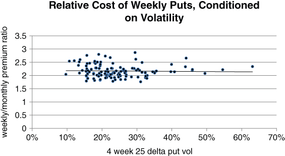
Figure 5.15 The relative cost of weekly puts is inelastic to the level of volatility
SUMMARY
It's a curious thing, but short- and long-dated options on the same asset have radically different characteristics. Short-dated OTM options are all about gamma. They're relatively cheap and insensitive to volatility, but offer tremendous potential when there are large realised moves. Weekly options benefit from contagion effects that tend to have the largest impact over short horizons. Conversely, long-dated OTM options reprice based on sentiment and do not have large direct dependence on price action.
The prescription, then, is to buy long-dated protection when investors are overconfident and short-dated options when you need an emergency hedge after an initial spike in volatility. From a hedging standpoint, medium-term options are the worst of both worlds and should generally be avoided.