
Chapter 13. Survival Analysis
Survival analysis is a way to describe how long things last. It is often used to study human lifetimes, but it also applies to “survival” of mechanical and electronic components, or more generally to intervals in time before an event.
If someone you know has been diagnosed with a life-threatening disease, you might have seen a “5-year survival rate,” which is the probability of surviving five years after diagnosis. That estimate and related statistics are the result of survival analysis.
The code in this chapter is in survival.py. For information about downloading and
working with this code, see Using the Code.
Survival Curves
The fundamental concept in survival analysis is the survival
curve, ![]() , which is a function that maps from a duration,
t, to the probability of surviving longer
than t. If you know the distribution of
durations, or “lifetimes”, finding the survival curve is easy; it’s just
the complement of the CDF:
, which is a function that maps from a duration,
t, to the probability of surviving longer
than t. If you know the distribution of
durations, or “lifetimes”, finding the survival curve is easy; it’s just
the complement of the CDF:
where ![]() is the probability of a lifetime less than or equal to
t.
is the probability of a lifetime less than or equal to
t.
For example, in the NSFG dataset, we know the duration of 11189 complete pregnancies. We can read this data and compute the CDF:
    preg = nsfg.ReadFemPreg()
    complete = preg.query('outcome in [1, 3, 4]').prglngth
    cdf = thinkstats2.Cdf(complete, label='cdf')
The outcome codes 1, 3, 4
indicate live birth, stillbirth, and miscarriage. For this analysis I am
excluding induced abortions, ectopic pregnancies, and pregnancies that
were in progress when the respondent was interviewed.
The DataFrame method query takes
a boolean expression and evaluates it for each row, selecting the rows
that yield True.
Figure 13-1 (top) shows the CDF of pregnancy length and its complement, the survival function. To represent the survival function, I define an object that wraps a Cdf and adapts the interface:
class SurvivalFunction(object):
    def __init__(self, cdf, label=''):
        self.cdf = cdf
        self.label = label or cdf.label

    @property
    def ts(self):
        return self.cdf.xs

    @property
    def ss(self):
        return 1 - self.cdf.ps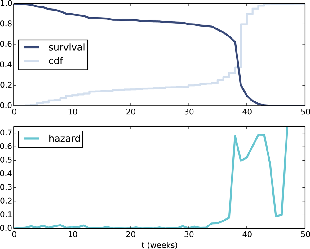
SurvivalFunction provides two
properties: ts, which is the sequence
of lifetimes, and ss, which is the
survival function. In Python, a “property” is a method that can be invoked as if it were a variable.
We can instantiate a SurvivalFunction by passing the CDF of
lifetimes:
sf = SurvivalFunction(cdf)
SurvivalFunction also provides
__getitem__ and Prob, which evaluate the survival
function:
# class SurvivalFunction

    def __getitem__(self, t):
        return self.Prob(t)

    def Prob(self, t):
        return 1 - self.cdf.Prob(t)
For example, sf[13] is the
fraction of pregnancies that proceed past the first trimester:
>>> sf[13]
0.86022
>>> cdf[13]
0.13978
About 86% of pregnancies proceed past the first trimester; about 14% do not.
SurvivalFunction provides
Render, so we can plot sf using the functions in thinkplot:
thinkplot.Plot(sf)
Figure 13-1 (top) shows the result. The curve is nearly flat between 13 and 26 weeks, which shows that few pregnancies end in the second trimester. And the curve is steepest around 39 weeks, which is the most common pregnancy length.
Hazard Function
From the survival function we can derive the hazard function; for pregnancy lengths, the hazard function maps from a time, t, to the fraction of pregnancies that continue until t and then end at t. To be more precise:
The numerator is the fraction of lifetimes that end at t, which is also ![]() .
.
SurvivalFunction provides
MakeHazard, which calculates the hazard
function:
# class SurvivalFunction

    def MakeHazard(self, label=''):
        ss = self.ss
        lams = {}
        for i, t in enumerate(self.ts[:-1]):
            hazard = (ss[i] - ss[i+1]) / ss[i]
            lams[t] = hazard

        return HazardFunction(lams, label=label)
The HazardFunction object is a
wrapper for a pandas Series:
class HazardFunction(object):

    def __init__(self, d, label=''):
        self.series = pandas.Series(d)
        self.label = label
d can be a dictionary or any
other type that can initialize a Series, including another Series.
label is a string used to identify the
HazardFunction when plotted.
HazardFunction provides __getitem__, so we can evaluate it
like this:
>>> hf = sf.MakeHazard()
>>> hf[39]
0.49689
So of all pregnancies that proceed until week 39, about 50% end in week 39.
Figure 13-1 (bottom) shows the hazard function for pregnancy lengths. For times after week 42, the hazard function is erratic because it is based on a small number of cases. Other than that the shape of the curve is as expected: it is highest around 39 weeks, and a little higher in the first trimester than in the second.
The hazard function is useful in its own right, but it is also an important tool for estimating survival curves, as we’ll see in the next section.
Estimating Survival Curves
If someone gives you the CDF of lifetimes, it is easy to compute the survival and hazard functions. But in many real-world scenarios, we can’t measure the distribution of lifetimes directly. We have to infer it.
For example, suppose you are following a group of patients to see how long they survive after diagnosis. Not all patients are diagnosed on the same day, so at any point in time, some patients have survived longer than others. If some patients have died, we know their survival times. For patients who are still alive, we don’t know survival times, but we have a lower bound.
If we wait until all patients are dead, we can compute the survival curve, but if we are evaluating the effectiveness of a new treatment, we can’t wait that long! We need a way to estimate survival curves using incomplete information.
As a more cheerful example, I will use NSFG data to quantify how long respondents “survive” until they get married for the first time. The range of respondents’ ages is 14 to 44 years, so the dataset provides a snapshot of women at different stages in their lives.
For women who have been married, the dataset includes the date of their first marriage and their age at the time. For women who have not been married, we know their age when interviewed, but have no way of knowing when or if they will get married.
Since we know the age at first marriage for some women, it might be tempting to exclude the rest and compute the CDF of the known data. That is a bad idea. The result would be doubly misleading: (1) older women would be overrepresented, because they are more likely to be married when interviewed, and (2) married women would be overrepresented! In fact, this analysis would lead to the conclusion that all women get married, which is obviously incorrect.
Kaplan-Meier Estimation
In this example it is not only desirable but necessary to include observations of unmarried women, which brings us to one of the central algorithms in survival analysis, Kaplan-Meier estimation.
The general idea is that we can use the data to estimate the hazard function, then convert the hazard function to a survival function. To estimate the hazard function, we consider, for each age, (1) the number of women who got married at that age and (2) the number of women “at risk” of getting married, which includes all women who were not married at an earlier age.
Here’s the code:
def EstimateHazardFunction(complete, ongoing, label=''):

    n = len(complete)
    hist_complete = thinkstats2.Hist(complete)
    sf_complete = SurvivalFunction(thinkstats2.Cdf(—complete))

    m = len(ongoing)
    sf_ongoing = SurvivalFunction(thinkstats2.Cdf(ongoing))

    lams = {}
    for t, ended in sorted(hist_complete.Items()):
        at_risk = ended + n * sf_complete[t] + m * sf_ongoing[t]
        lams[t] = ended / at_risk

    return HazardFunction(lams, label=label)
complete is the set of complete
observations; in this case, the ages when respondents got married.
ongoing is the set of incomplete
observations; that is, the ages of unmarried women when they were
interviewed.
First, we precompute hist_complete, which is the Hist of ages when women
were married, sf_complete,
the survival function for married women, and sf_ongoing, the survival function for unmarried
women.
The loop iterates through the ages when respondents got married. For
each value of t, we have ended, which is the number of women who got
married at age t. Then we compute the
number of women “at risk”, which is the sum of:
ended, the number of respondents married at aget,n * sf_complete[t], the number of respondents married after aget.m * sf_ongoing[t], the number of unmarried respondents interviewed aftert, and therefore known not to have been married at or beforet.
The estimated value of the hazard function at t is the ratio of ended to at_risk.
lams is a dictionary that maps
from t to ![]() . The result is a
. The result is a HazardFunction object.
The Marriage Curve
To test this function, we have to do some data cleaning and transformation. The NSFG variables we need are:
cmbirthcmintvwThe date the respondent was interviewed, known for all respondents.
cmmarrhxThe date the respondent was first married, if applicable and known.
evrmarryThis is 1 if the respondent had been married prior to the date of interview; otherwise, 0.
The first three variables are encoded in “century-months”; that is, the integer number of months since December 1899. So century-month 1 is January 1900.
First, we read the respondent file and replace invalid values of
cmmarrhx:
    resp = chap01soln.ReadFemResp()
    resp.cmmarrhx.replace([9997, 9998, 9999], np.nan, inplace=True)
Then we compute each respondent’s age when married and age when interviewed:
    resp['agemarry'] = (resp.cmmarrhx - resp.cmbirth) / 12.0
    resp['age'] = (resp.cmintvw - resp.cmbirth) / 12.0
Next we extract complete, which
is the age at marriage for women who have been married, and ongoing, which is the age at interview for women
who have not:
    complete = resp[resp.evrmarry==1].agemarry
    ongoing = resp[resp.evrmarry==0].age
Finally we compute the hazard function.
hf = EstimateHazardFunction(complete, ongoing)
Figure 13-2 (top) shows the estimated hazard function; it is low in the teens, higher in the 20s, and declining in the 30s. It increases again in the 40s, but that is an artifact of the estimation process; as the number of respondents “at risk” decreases, a small number of women getting married yields a large estimated hazard. The survival function will smooth out this noise.
Estimating the Survival Function
Once we have the hazard function, we can estimate the survival function. The
chance of surviving past time t is the
chance of surviving all times up through t, which is the cumulative product of the
complementary hazard function:

The HazardFunction class provides
MakeSurvival, which computes this
product:
# class HazardFunction:

    def MakeSurvival(self):
        ts = self.series.index
        ss = (1 - self.series).cumprod()
        cdf = thinkstats2.Cdf(ts, 1-ss)
        sf = SurvivalFunction(cdf)
        return sf
ts is the sequence of times where
the hazard function is estimated. ss is
the cumulative product of the complementary hazard function, so it is the
survival function.
Because of the way SurvivalFunction is implemented, we have to
compute the complement of ss, make a
Cdf, and then instantiate a SurvivalFunction object.
Figure 13-2 (bottom) shows the result. The survival curve is steepest between 25 and 35, when most women get married. Between 35 and 45, the curve is nearly flat, indicating that women who do not marry before age 35 are unlikely to get married.
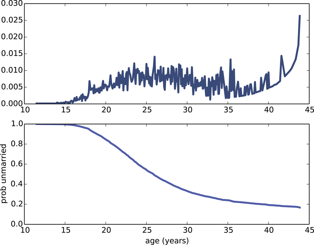
A curve like this was the basis of a famous magazine article in 1986; Newsweek reported that a 40-year old unmarried woman was “more likely to be killed by a terrorist” than get married. These statistics were widely reported and became part of popular culture, but they were wrong then (because they were based on faulty analysis) and turned out to be even more wrong (because of cultural changes that were already in progress and continued). In 2006, Newsweek ran an another article admitting that they were wrong.
I encourage you to read more about this article, the statistics it was based on, and the reaction. It should remind you of the ethical obligation to perform statistical analysis with care, interpret the results with appropriate skepticism, and present them to the public accurately and honestly.
Confidence Intervals
Kaplan-Meier analysis yields a single estimate of the survival curve, but it is also important to quantify the uncertainty of the estimate. As usual, there are three possible sources of error: measurement error, sampling error, and modeling error.
In this example, measurement error is probably small. People generally know when they were born, whether they’ve been married, and when. And they can be expected to report this information accurately.
We can quantify sampling error by resampling. Here’s the code:
def ResampleSurvival(resp, iters=101):
    low, high = resp.agemarry.min(), resp.agemarry.max()
    ts = np.arange(low, high, 1/12.0)

    ss_seq = []
    for i in range(iters):
        sample = thinkstats2.ResampleRowsWeighted(resp)
        hf, sf = EstimateSurvival(sample)
        ss_seq.append(sf.Probs(ts))

    low, high = thinkstats2.PercentileRows(ss_seq, [5, 95])
    thinkplot.FillBetween(ts, low, high)
ResampleSurvival takes resp, a DataFrame of respondents, and iters,
the number of times to resample. It computes ts, which is the sequence of ages where we will
evaluate the survival functions.
Inside the loop, ResampleSurvival:
Resamples the respondents using
ResampleRowsWeighted, which we saw in Weighted Resampling.Calls
EstimateSurvival, which uses the process in the previous sections to estimate the hazard and survival curves, andEvaluates the survival curve at each age in
ts.
ss_seq is a sequence
of evaluated survival curves. PercentileRows takes this sequence and computes
the 5th and 95th percentiles, returning a 90% confidence interval for the
survival curve.
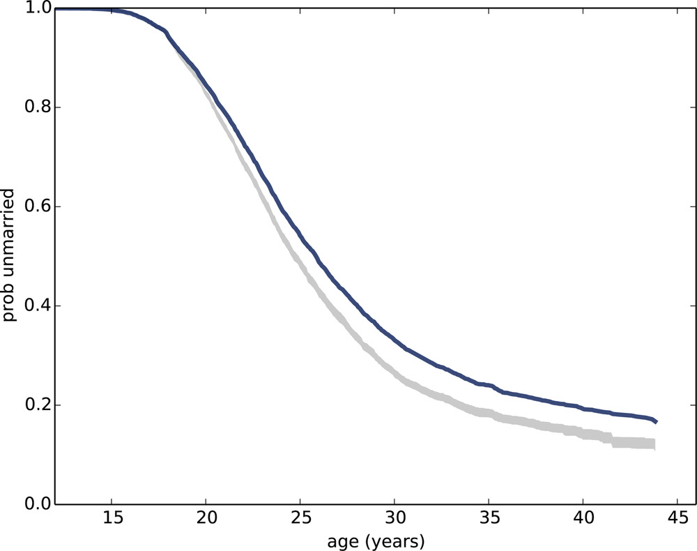
Figure 13-3 shows the result along with the survival function we estimated in the previous section. The confidence interval takes into account the sampling weights, unlike the estimated curve. The discrepancy between them indicates that the sampling weights have a substantial effect on the estimate—we will have to keep that in mind.
Cohort Effects
One of the challenges of survival analysis is that different parts of the estimated curve are based on
different groups of respondents. The part of the curve at time t is based on respondents whose age was at least
t when they were interviewed. So the
leftmost part of the curve includes data from all respondents, but the
rightmost part includes only the oldest respondents.
If the relevant characteristics of the respondents are not changing over time, that’s fine, but in this case it seems likely that marriage patterns are different for women born in different generations. We can investigate this effect by grouping respondents according to their decade of birth. Groups like this, defined by date of birth or similar events, are called cohorts, and differences between the groups are called cohort effects.
To investigate cohort effects in the NSFG marriage data, I gathered the Cycle 6 data from 2002 used throughout this book; the Cycle 7 data from 2006–2010 used in Replication; and the Cycle 5 data from 1995. In total these datasets include 30,769 respondents.
    resp5 = ReadFemResp1995()
    resp6 = ReadFemResp2002()
    resp7 = ReadFemResp2010()
    resps = [resp5, resp6, resp7]
For each DataFrame, resp, I use
cmbirth to compute the decade of birth
for each respondent:
    month0 = pandas.to_datetime('1899-12-15')
    dates = [month0 + pandas.DateOffset(months=cm)
             for cm in resp.cmbirth]
    resp['decade'] = (pandas.DatetimeIndex(dates).year - 1900) // 10
cmbirth is encoded as the integer
number of months since December 1899; month0 represents that date as a Timestamp
object. For each birth date, we instantiate a DateOffset that contains the century-month and
add it to month0; the result is a
sequence of Timestamps, which is converted to a DateTimeIndex. Finally, we extract year and compute decades.
To take into account the sampling weights, and also to show variability due to sampling error, I resample the data, group respondents by decade, and plot survival curves:
    for i in range(iters):
        samples = [thinkstats2.ResampleRowsWeighted(resp)
                   for resp in resps]
        sample = pandas.concat(samples, ignore_index=True)
        groups = sample.groupby('decade')

        EstimateSurvivalByDecade(groups, alpha=0.2)
Data from the three NSFG cycles use different sampling weights, so I
resample them separately and then use concat to merge them into a single DataFrame.
The parameter ignore_index
tells concat not to match up
respondents by index; instead it creates a new index from 0 to
30768.
EstimateSurvivalByDecade plots
survival curves for each cohort:
def EstimateSurvivalByDecade(resp):
    for name, group in groups:
        hf, sf = EstimateSurvival(group)
        thinkplot.Plot(sf)
Figure 13-4 shows the results.
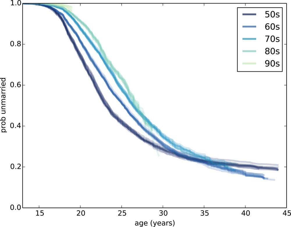
Several patterns are visible:
Women born in the 1950s married earliest, with successive cohorts marrying later and later, at least until age 30 or so.
Women born in the 1960s follow a surprising pattern. Prior to age 25, they were marrying at slower rates than their predecessors. After age 25, they were marrying faster. By age 32, they had overtaken the 50s cohort, and at age 44 they are substantially more likely to have married.
Women born in the 60s turned 25 between 1985 and 1995. Remembering that the Newsweek article I mentioned was published in 1986, it is tempting to imagine that the article triggered a marriage boom. That explanation would be too pat, but it is possible that the article and the reaction to it were indicative of a mood that affected the behavior of this cohort.
The pattern of the 1970s cohort is similar. They are less likely than their predecessors to be married before age 25, but at age 35 they have caught up with both of the previous cohorts.
Women born in the 1980s are even less likely to marry before age 25. What happens after that is not clear; for more data, we have to wait for the next cycle of the NSFG.
Extrapolation
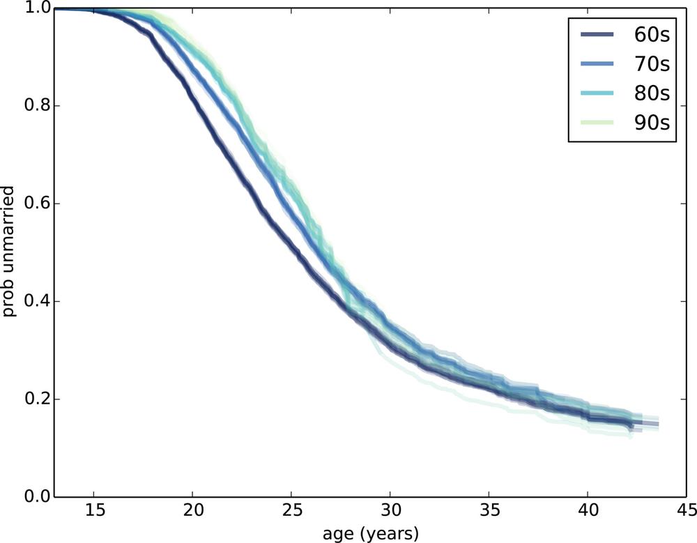
The survival curve for the ’70s cohort ends at about age 38; for the ’80s cohort it ends at age 28, and for the ’90s cohort we hardly have any data at all.
We can extrapolate these curves by “borrowing” data from the
previous cohort. HazardFunction provides a method, Extend, that copies the tail from another longer
HazardFunction:
# class HazardFunction

    def Extend(self, other):
        last = self.series.index[-1]
        more = other.series[other.series.index > last]
        self.series = pandas.concat([self.series, more])
As we saw in Hazard Function, the HazardFunction contains
a Series that maps from t to
![]() .
. Extend finds
last, which is the last index in
self.series, selects values from
other that come later than last, and appends them onto self.series.
Now we can extend the HazardFunction for each cohort, using values from the predecessor:
def PlotPredictionsByDecade(groups):
    hfs = []
    for name, group in groups:
        hf, sf = EstimateSurvival(group)
        hfs.append(hf)

    thinkplot.PrePlot(len(hfs))
    for i, hf in enumerate(hfs):
        if i > 0:
            hf.Extend(hfs[i-1])
        sf = hf.MakeSurvival()
        thinkplot.Plot(sf)
groups is a GroupBy object with
respondents grouped by decade of birth. The first loop computes the
HazardFunction for each group.
The second loop extends each HazardFunction with values from its predecessor, which might contain values from the previous group, and so on. Then it converts each HazardFunction to a SurvivalFunction and plots it.
Figure 13-5 shows the results; I’ve removed the 50s cohort to make the predictions more visible. These results suggest that by age 40, the most recent cohorts will converge with the 60s cohort, with fewer than 20% never married.
Expected Remaining Lifetime
Given a survival curve, we can compute the expected remaining lifetime as a function of current age. For example, given the survival function of pregnancy length from Survival Curves, we can compute the expected time until delivery.
The first step is to extract the PMF of lifetimes. SurvivalFunction provides a method that does
that:
# class SurvivalFunction

    def MakePmf(self, filler=None):
        pmf = thinkstats2.Pmf()
        for val, prob in self.cdf.Items():
            pmf.Set(val, prob)

        cutoff = self.cdf.ps[-1]
        if filler is not None:
            pmf[filler] = 1-cutoff

        return pmf
Remember that the SurvivalFunction contains the Cdf of lifetimes. The loop copies the values and probabilities from the Cdf into a Pmf.
cutoff is the highest probability
in the Cdf, which is 1 if the Cdf is complete, and otherwise less than 1.
If the Cdf is incomplete, we plug in the provided value, filler, to cap it off.
The Cdf of pregnancy lengths is complete, so we don’t have to worry about this detail yet.
The next step is to compute the expected remaining lifetime, where
“expected” means average. SurvivalFunction provides a method that does
that, too:
# class SurvivalFunction

    def RemainingLifetime(self, filler=None, func=thinkstats2.Pmf.Mean):
        pmf = self.MakePmf(filler=filler)
        d = {}
        for t in sorted(pmf.Values())[:-1]:
            pmf[t] = 0
            pmf.Normalize()
            d[t] = func(pmf) - t

        return pandas.Series(d)
RemainingLifetime takes filler, which is passed along to MakePmf, and func which is the function used to summarize the
distribution of remaining lifetimes.
pmf is the Pmf of lifetimes
extracted from the SurvivalFunction. d
is a dictionary that contains the results, a map from current age,
t, to expected remaining
lifetime.
The loop iterates through the values in the Pmf. For each value of
t it computes the conditional
distribution of lifetimes, given that the lifetime exceeds t. It does that by removing values from the Pmf
one at a time and renormalizing the remaining values.
Then it uses func to summarize
the conditional distribution. In this example the result is the mean
pregnancy length, given that the length exceeds t. By subtracting t we get the mean remaining pregnancy
length.
Figure 13-6 (left) shows the expected remaining pregnancy length as a function of the current duration. For example, during Week 0, the expected remaining duration is about 34 weeks. That’s less than full term (39 weeks) because terminations of pregnancy in the first trimester bring the average down.
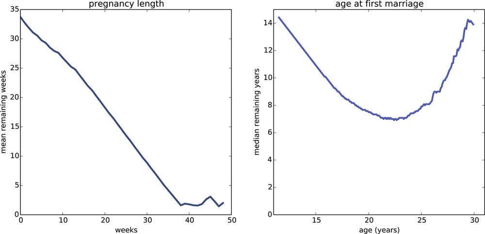
The curve drops slowly during the first trimester. After 13 weeks, the expected remaining lifetime has dropped by only 9 weeks, to 25. After that the curve drops faster, by about a week per week.
Between Week 37 and 42, the curve levels off between 1 and 2 weeks. At any time during this period, the expected remaining lifetime is the same; with each week that passes, the destination gets no closer. Processes with this property are called memoryless because the past has no effect on the predictions. This behavior is the mathematical basis of the infuriating mantra of obstetrics nurses: “any day now.”
Figure 13-6 (right) shows the median remaining time until first marriage, as a function of age. For an 11 year-old girl, the median time until first marriage is about 14 years. The curve decreases until age 22 when the median remaining time is about 7 years. After that it increases again: by age 30 it is back where it started, at 14 years.
Based on this data, young women have decreasing remaining “lifetimes”. Mechanical components with this property are called NBUE for “new better than used in expectation,” meaning that a new part is expected to last longer.
Women older than 22 have increasing remaining time until first marriage. Components with this property are called UBNE for “used better than new in expectation.” That is, the older the part, the longer it is expected to last. Newborns and cancer patients are also UBNE; their life expectancy increases the longer they live.
For this example I computed median, rather than mean, because the Cdf is incomplete; the survival curve projects that about 20% of respondents will not marry before age 44. The age of first marriage for these women is unknown, and might be non-existent, so we can’t compute a mean.
I deal with these unknown values by replacing them with np.inf, a special value that represents
infinity. That makes the mean infinity for all ages, but the median is
well-defined as long as more than 50% of the remaining lifetimes are
finite, which is true until age 30. After that it is hard to define a
meaningful expected remaining lifetime.
Here’s the code that computes and plots these functions:
    rem_life1 = sf1.RemainingLifetime()
    thinkplot.Plot(rem_life1)

    func = lambda pmf: pmf.Percentile(50)
    rem_life2 = sf2.RemainingLifetime(filler=np.inf, func=func)
    thinkplot.Plot(rem_life2)
sf1 is the survival function for
pregnancy length; in this case we can use the default values for RemainingLifetime.
sf2 is the survival function for
age at first marriage; func is a
function that takes a Pmf and computes its median (50th percentile).
Exercises
My solution to this exercise is in chap13soln.py.
In NSFG Cycles 6 and 7, the variable cmdivorcx contains the date of divorce for the
respondent’s first marriage, if applicable, encoded in
century-months.
Compute the duration of marriages that have ended in divorce, and the duration, so far, of marriages that are ongoing. Estimate the hazard and survival function for the duration of marriage.
Use resampling to take into account sampling weights, and plot data from several resamples to visualize sampling error.
Consider dividing the respondents into groups by decade of birth, and possibly by age at first marriage.
Glossary
- survival analysis
A set of methods for describing and predicting lifetimes, or more generally time until an event occurs.
- survival curve
A function that maps from a time, t, to the probability of surviving past t.
- hazard function
A function that maps from t to the fraction of people alive until t who die at t.
- Kaplan-Meier estimation
- cohort
a group of subjects defined by an event, like date of birth, in a particular interval of time.
- cohort effect
- NBUE
A property of expected remaining lifetime, “New better than used in expectation.”
- UBNE
A property of expected remaining lifetime, “Used better than new in expectation.”