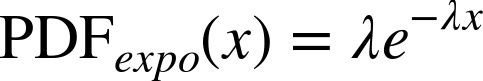
The derivative of a CDF is called a probability density function, or PDF. For example, the PDF of an exponential distribution is

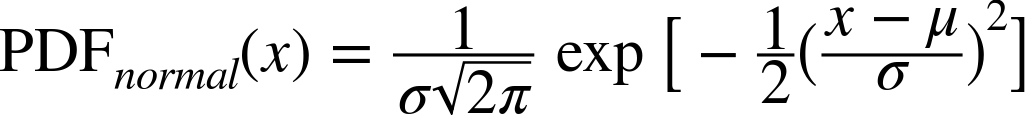
The PDF of a normal distribution is

Evaluating a PDF for a particular value of x is usually not useful. The result is not a probability; it is a probability density.

In physics, density is mass per unit of volume; in order to get a mass, you have to multiply by volume or, if the density is not constant, you have to integrate over volume.

Similarly, probability density measures probability per unit of x. In order to get a probability mass, you have to integrate over x.

thinkstats2 provides a class called Pdf that represents a probability density function. Every Pdf object provides the following methods:

Pdf is an abstract parent class, which means you should not instantiate it; that is, you cannot create a Pdf object. Instead, you should define a child class that inherits from Pdf and provides definitions of Density and GetLinspace. Pdf provides Render and MakePmf.

For example, thinkstats2 provides a class named NormalPdf that evaluates the normal density function.

class NormalPdf(Pdf):

    def __init__(self, mu=0, sigma=1, label=''):
        self.mu = mu
        self.sigma = sigma
        self.label = label

    def Density(self, xs):
        return scipy.stats.norm.pdf(xs, self.mu, self.sigma)

    def GetLinspace(self):
        low, high = self.mu-3*self.sigma, self.mu+3*self.sigma
        return np.linspace(low, high, 101)

The NormalPdf object contains the parameters mu and sigma. Density uses scipy.stats.norm, which is an object that represents a normal distribution and provides cdf and pdf, among other methods (see The Normal Distribution).

The following example creates a NormalPdf with the mean and variance of adult female heights, in cm, from the BRFSS (see The lognormal Distribution). Then it computes the density of the distribution at a location one standard deviation from the mean.

>>> mean, var = 163, 52.8
>>> std = math.sqrt(var)
>>> pdf = thinkstats2.NormalPdf(mean, std)
>>> pdf.Density(mean + std)
0.0333001

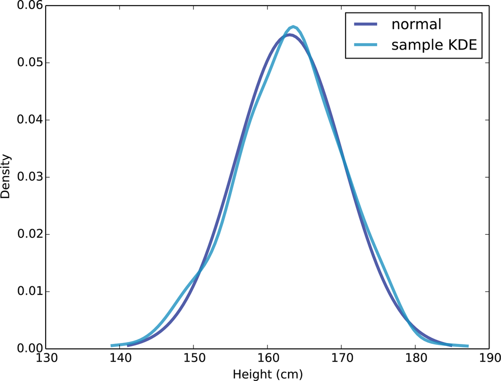
The result is about 0.03, in units of probability mass per cm. Again, a probability density doesn’t mean much by itself. But if we plot the Pdf, we can see the shape of the distribution:

>>> thinkplot.Pdf(pdf, label='normal')
>>> thinkplot.Show()

thinkplot.Pdf plots the Pdf as a smooth function, as contrasted with thinkplot.Pmf, which renders a Pmf as a step function. Figure 6-1 shows the result, as well as a PDF estimated from a sample, which we’ll compute in the next section.

Figure 6-1. A normal PDF that models adult female height in the US, and the kernel density estimate of a sample with .

You can use MakePmf to approximate the Pdf:

>>> pmf = pdf.MakePmf()

By default, the resulting Pmf contains 101 points equally spaced from mu - 3*sigma to mu + 3*sigma. Optionally, MakePmf and Render can take keyword arguments low, high, and n.

Kernel density estimation (KDE) is an algorithm that takes a sample and finds an appropriately smooth PDF that fits the data. You can read details at Wikipedia.

scipy provides an implementation of KDE and thinkstats2 provides a class called EstimatedPdf that uses it:

class EstimatedPdf(Pdf):

    def __init__(self, sample):
        self.kde = scipy.stats.gaussian_kde(sample)

    def Density(self, xs):
        return self.kde.evaluate(xs)

__init__ takes a sample and computes a kernel density estimate. The result is a gaussian_kde object that provides an evaluate method.

Density takes a value or sequence, calls gaussian_kde.evaluate, and returns the resulting density. The word “Gaussian” appears in the name because it uses a filter based on a Gaussian distribution to smooth the KDE.

Here’s an example that generates a sample from a normal distribution and then makes an EstimatedPdf to fit it:

>>> sample = [random.gauss(mean, std) for i in range(500)]
>>> sample_pdf = thinkstats2.EstimatedPdf(sample)
>>> thinkplot.Pdf(pdf, label='sample KDE')

sample is a list of 500 random heights. sample_pdf is a Pdf object that contains the estimated KDE of the sample. pmf is a Pmf object that approximates the Pdf by evaluating the density at a sequence of equally spaced values.

Figure 6-1 shows the normal density function and a KDE based on a sample of 500 random heights. The estimate is a good match for the original distribution.

Estimating a density function with KDE is useful for several purposes:

At this point we have seen PMFs, CDFs and PDFs; let’s take a minute to review. Figure 6-2 shows how these functions relate to each other.

Figure 6-2. A framework that relates representations of distribution functions

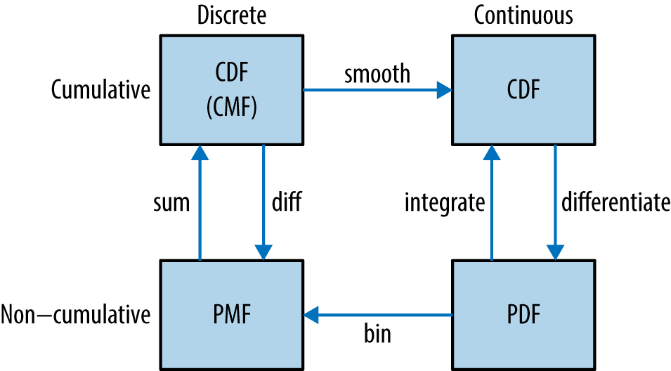
We started with PMFs, which represent the probabilities for a discrete set of values. To get from a PMF to a CDF, you add up the probability masses to get cumulative probabilities. To get from a CDF back to a PMF, you compute differences in cumulative probabilities. We’ll see the implementation of these operations in the next few sections.

A PDF is the derivative of a continuous CDF; or, equivalently, a CDF is the integral of a PDF. Remember that a PDF maps from values to probability densities; to get a probability, you have to integrate.

To get from a discrete to a continuous distribution, you can perform various kinds of smoothing. One form of smoothing is to assume that the data come from an analytic continuous distribution (like exponential or normal) and to estimate the parameters of that distribution. Another option is kernel density estimation.

The opposite of smoothing is discretizing, or quantizing. If you evaluate a PDF at discrete points, you can generate a PMF that is an approximation of the PDF. You can get a better approximation using numerical integration.

To distinguish between continuous and discrete CDFs, it might be better for a discrete CDF to be a “cumulative mass function,” but as far as I can tell no one uses that term.

At this point you should know how to use the basic types provided by thinkstats2: Hist, Pmf, Cdf, and Pdf. The next few sections provide details about how they are implemented. This material might help you use these classes more effectively, but it is not strictly necessary.

Hist and Pmf inherit from a parent class called _DictWrapper. The leading underscore indicates that this class is “internal”; that is, it should not be used by code in other modules. The name indicates what it is: a dictionary wrapper. Its primary attribute is d, the dictionary that maps from values to their frequencies.

The values can be any hashable type. The frequencies should be integers, but can be any numeric type.

_DictWrapper contains methods appropriate for both Hist and Pmf, including __init__, Values, Items and Render. It also provides modifier methods Set, Incr, Mult, and Remove. These methods are all implemented with dictionary operations. For example:

# class _DictWrapper

    def Incr(self, x, term=1):
        self.d[x] = self.d.get(x, 0) + term

    def Mult(self, x, factor):
        self.d[x] = self.d.get(x, 0) * factor

    def Remove(self, x):
        del self.d[x]

Hist also provides Freq, which looks up the frequency of a given value.

Because Hist operators and methods are based on dictionaries, these methods are constant time operations; that is, their runtime does not increase as the Hist gets bigger.

Pmf and Hist are almost the same thing, except that a Pmf maps values to floating-point probabilities, rather than integer frequencies. If the sum of the probabilities is 1, the Pmf is normalized.

Pmf provides Normalize, which computes the sum of the probabilities and divides through by a factor:

# class Pmf

    def Normalize(self, fraction=1.0):
        total = self.Total()
        if total == 0.0:
            raise ValueError('Total probability is zero.')

        factor = float(fraction) / total
        for x in self.d:
            self.d[x] *= factor

        return total

fraction determines the sum of the probabilities after normalizing; the default value is 1. If the total probability is 0, the Pmf cannot be normalized, so Normalize raises ValueError.

Hist and Pmf have the same constructor. It can take as an argument a dict, Hist, Pmf or Cdf, a pandas Series, a list of (value, frequency) pairs, or a sequence of values.

If you instantiate a Pmf, the result is normalized. If you instantiate a Hist, it is not. To construct an unnormalized Pmf, you can create an empty Pmf and modify it. The Pmf modifiers do not renormalize the Pmf.

A CDF maps from values to cumulative probabilities, so I could have implemented Cdf as a _DictWrapper. But the values in a CDF are ordered and the values in a _DictWrapper are not. Also, it is often useful to compute the inverse CDF; that is, the map from cumulative probability to value. So the implementaion I chose is two sorted lists. That way I can use binary search to do a forward or inverse lookup in logarithmic time.

The Cdf constructor can take as a parameter a sequence of values or a pandas Series, a dictionary that maps from values to probabilities, a sequence of (value, probability) pairs, a Hist, Pmf, or Cdf. Or if it is given two parameters, it treats them as a sorted sequence of values and the sequence of corresponding cumulative probabilities.

Given a sequence, pandas Series, or dictionary, the constructor makes a Hist. Then it uses the Hist to initialize the attributes:

        self.xs, freqs = zip(*sorted(dw.Items()))
        self.ps = np.cumsum(freqs, dtype=np.float)
        self.ps /= self.ps[-1]

xs is the sorted list of values; freqs is the list of corresponding frequencies. np.cumsum computes the cumulative sum of the frequencies. Dividing through by the total frequency yields cumulative probabilities. For n values, the time to construct the Cdf is proportional to .

Here is the implementation of Prob, which takes a value and returns its cumulative probability:

# class Cdf
    def Prob(self, x):
        if x < self.xs[0]:
            return 0.0
        index = bisect.bisect(self.xs, x)
        p = self.ps[index - 1]
        return p

The bisect module provides an implementation of binary search. And here is the implementation of Value, which takes a cumulative probability and returns the corresponding value:

# class Cdf
    def Value(self, p):
        if p < 0 or p > 1:
            raise ValueError('p must be in range [0, 1]')

        index = bisect.bisect_left(self.ps, p)
        return self.xs[index]

Given a Cdf, we can compute the Pmf by computing differences between consecutive cumulative probabilities. If you call the Cdf constructor and pass a Pmf, it computes differences by calling Cdf.Items:

# class Cdf
    def Items(self):
        a = self.ps
        b = np.roll(a, 1)
        b[0] = 0
        return zip(self.xs, a-b)

np.roll shifts the elements of a to the right, and “rolls” the last one back to the beginning. We replace the first element of b with 0 and then compute the difference a-b. The result is a NumPy array of probabilities.

Cdf provides Shift and Scale, which modify the values in the Cdf, but the probabilities should be treated as immutable.

Any time you take a sample and reduce it to a single number, that number is a statistic. The statistics we have seen so far include mean, variance, median, and interquartile range.

A raw moment is a kind of statistic. If you have a sample of values, x_i, the kth raw moment is:

Or if you prefer Python notation:

def RawMoment(xs, k):
    return sum(x**k for x in xs) / len(xs)

When the result is the sample mean, . The other raw moments don’t mean much by themselves, but they are used in some computations.

The central moments are more useful. The kth central moment is:

Or in Python:

def CentralMoment(xs, k):
    mean = RawMoment(xs, 1)
    return sum((x - mean)**k for x in xs) / len(xs)

When the result is the second central moment, which you might recognize as variance. The definition of variance gives a hint about why these statistics are called moments. If we attach a weight along a ruler at each location, x_i, and then spin the ruler around the mean, the moment of inertia of the spinning weights is the variance of the values. If you are not familiar with moment of inertia, see Wikipedia..

When you report moment-based statistics, it is important to think about the units. For example, if the values x_i are in cm, the first raw moment is also in cm. But the second moment is in cm², the third moment is in cm³, and so on.

Because of these units, moments are hard to interpret by themselves. That’s why, for the second moment, it is common to report standard deviation, which is the square root of variance, so it is in the same units as x_i.

Skewness is a property that describes the shape of a distribution. If the distribution is symmetric around its central tendency, it is unskewed. If the values extend farther to the right, it is “right skewed” and if the values extend left, it is “left skewed.”

This use of “skewed” does not have the usual connotation of “biased.” Skewness only describes the shape of the distribution; it says nothing about whether the sampling process might have been biased.

Several statistics are commonly used to quantify the skewness of a distribution. Given a sequence of values, x_i, the sample skewness, g₁, can be computed like this:

def StandardizedMoment(xs, k):
    var = CentralMoment(xs, 2)
    std = math.sqrt(var)
    return CentralMoment(xs, k) / std**k

def Skewness(xs):
    return StandardizedMoment(xs, 3)

g₁ is the third standardized moment, which means that it has been normalized so it has no units.

Negative skewness indicates that a distribution skews left; positive skewness indicates that a distribution skews right. The magnitude of g₁ indicates the strength of the skewness, but by itself it is not easy to interpret.

In practice, computing sample skewness is usually not a good idea. If there are any outliers, they have a disproportionate effect on g₁.

Another way to evaluate the asymmetry of a distribution is to look at the relationship between the mean and the median. Extreme values have more effect on the mean than the median, so in a distribution that skews left, the mean is less than the median. In a distribution that skews right, the mean is greater.

Pearson’s median skewness coefficient is a measure of skewness based on the difference between the sample mean and median:

Where is the sample mean, m is the median, and S is the standard deviation. Or in Python:

def Median(xs):
    cdf = thinkstats2.MakeCdfFromList(xs)
    return cdf.Value(0.5)

def PearsonMedianSkewness(xs):
    median = Median(xs)
    mean = RawMoment(xs, 1)
    var = CentralMoment(xs, 2)
    std = math.sqrt(var)
    gp = 3 * (mean - median) / std
    return gp

This statistic is robust, which means that it is less vulnerable to the effect of outliers.

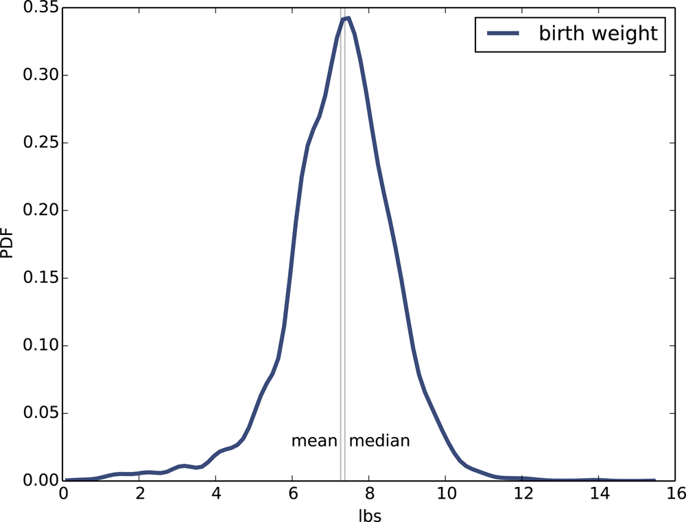
As an example, let’s look at the skewness of birth weights in the NSFG pregnancy data. Here’s the code to estimate and plot the PDF:

    live, firsts, others = first.MakeFrames()
    data = live.totalwgt_lb.dropna()
    pdf = thinkstats2.EstimatedPdf(data)
    thinkplot.Pdf(pdf, label='birth weight')

Figure 6-3 shows the result. The left tail appears longer than the right, so we suspect the distribution is skewed left. The mean, 7.27 lbs, is a bit less than the median, 7.38 lbs, so that is consistent with left skew. And both skewness coefficients are negative: sample skewness is -0.59; Pearson’s median skewness is -0.23.

Figure 6-3. Estimated PDF of birthweight data from the NSFG

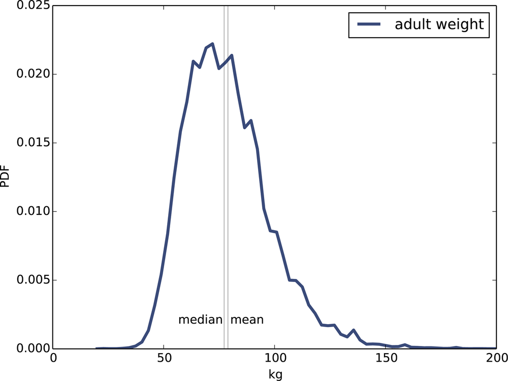
Now let’s compare this distribution to the distribution of adult weight in the BRFSS. Again, here’s the code:

    df = brfss.ReadBrfss(nrows=None)
    data = df.wtkg2.dropna()
    pdf = thinkstats2.EstimatedPdf(data)
    thinkplot.Pdf(pdf, label='adult weight')

Figure 6-4 shows the result. The distribution appears skewed to the right. Sure enough, the mean, 79.0, is bigger than the median, 77.3. The sample skewness is 1.1 and Pearson’s median skewness is 0.26.

Figure 6-4. Estimated PDF of adult weight data from the BRFSS.

The sign of the skewness coefficient indicates whether the distribution skews left or right, but other than that, they are hard to interpret. Sample skewness is less robust; that is, it is more susceptible to outliers. As a result it is less reliable when applied to skewed distributions, exactly when it would be most relevant.

Pearson’s median skewness is based on a computed mean and variance, so it is also susceptible to outliers, but since it does not depend on a third moment, it is somewhat more robust.

A solution to this exercise is in chap06soln.py.