
Chapter 4
Computational techniques
Abstract
This chapter gives an introduction to a number of computational techniques that are used in the study of train aerodynamics. Firstly, the range of analytical and numerical techniques used in train aerodynamics is described. Simple panel methods are then outlined and their historic and continuing utility discussed. The use of the Reynolds-averaged Navier–Stokes (RANS) equations is then discussed at some length. The representation of turbulence in this approach is presented, and a range of turbulence viscosity models are discussed. Reynolds stress models and unsteady RANS methods are briefly described. Direct numerical simulation (DNS) of the Navier–Stokes equations is then considered, and it is shown that a direct application of this approach to train aerodynamics is not currently possible. Hybrid models are then discussed (large eddy simulation (LES) and detached eddy simulation (DES), which use DNS for the calculation of large turbulence scales and turbulence models of different sorts for small turbulence scales or near flow boundaries. The Lattice Boltzmann (LB) approach is then set out, which solves the Boltzmann equation rather than the Navier–Stokes equations, and is used in a similar manner to LES. Finally, a range of numerical optimisation techniques are presented.
Keywords
CFD; DES; DNS; LES; Optimisation techniques; Panel methods; RANS; Turbulence models
4.1. Analytical and computational methods in train aerodynamics
In this chapter we consider a range of numerical techniques that are used in the study of train aerodynamics. In the main, these techniques are based on the Navier–Stokes equations, which can, in principle, be solved for any particular flow geometry. Eqs. 2.1–2.3 set out the two-dimensional unsteady form of these equations, and the incompressible form is presented in Eqs. 2.4–2.6. These equations are closed, i.e., if solved for given boundary and initial conditions, they lead to the pressure and velocity fields in both time and space. However, they are second-order nonlinear partial differential equations and it is only possible to solve these equations analytically for simple flow cases.
That point being made, there are some simple analytical techniques that are of use in the study of train aerodynamics. For example, boundary layer methods based on the boundary layer equations of Section 2.8 can be useful in understanding the flow along the sides and roofs of trains (Sterling et al., 2008) (see Chapter 5). A more complex, but still analytical, boundary layer solution for flow between two moving walls, a Couette flow, will be used in Chapter 9 to consider the underbody flow field and the movement of ballast (Garcia et al., 2011). Analytical potential flow methods (Section 2.9) have been used to predict the flow field around simple train nose shapes and the associated forces on trackside infrastructure, and these will be briefly discussed in Chapter 8 where loads on trackside structures are considered (Sanz-Andres et al., 2004a, 2004b; Barrero-Gil and Sanz-Andres, 2009). The main use of such analytical models is to identify the basic physics of the flow, to help develop a basic understanding of the issues involved and to act as a framework for the consideration of experimental results.
The simplest numerical solutions, for incompressible inviscid flows such as those around train noses, are also based on potential flow solutions to the equations of motions, in particular, the range of techniques known as panel methods. These methods will be presented in Section 4.2.
The alternative, more complex, way of solving the equations of motion is to appropriately linearise them and then solve the resulting system of linear equations using high-performance computers. This approach has come to be known generically as computational fluid dynamics (CFD). To solve these equations numerically, the first step is to define the computational domain in which to solve for the velocity and pressure fields. The flow conditions at the boundaries of the domain are called the boundary conditions. The computational domain is then discretized into a finite number of computational cells and the solution is obtained for each cell. The linearised form of the governing equations requires that the size of the computational cell is very small, and the flow variables are effectively averaged in space over the computational cell.
There are two approaches for numerically solving the resulting governing equations. The first approach is to average these equations in time and then to solve the resulting equations (Eqs. 2.7–2.9) for each cell. This approach effectively damps out the turbulent fluctuations in time, and no turbulent scales are resolved. This approach is called Reynolds-averaged Navier–Stokes (RANS). By averaging over short time periods, this approach can be extended to capture large-scale unsteady flows using unsteady RANS (URANS). These methods, which are very widely used for all aspects of train aerodynamics, are discussed in Section 4.3.
The other approach is to solve the governing equations directly to resolve all the turbulent scales in the flow. This approach is called direct numerical simulation (DNS). As the spatial averaging associated with the computational grid in such methods means that only turbulent scales larger than the averaging space (or filter width) are resolved, for full DNS the computational cells have to very small, and the resources required for any practical calculations are prohibitively high. Thus the effect of the turbulent scales smaller than the filter width is usually modelled using simple turbulence models. This leads to one approach that solves the full unsteady equations of motion for large turbulence scales, but relies on modelling of the small turbulence scales (large eddy simulation – LES), and to a further approach that uses LES for most of the flow field and RANS-based methods for regions near flow boundaries (detached eddy simulation – DES). These methods are described in Section 4.4.
In Section 4.5, a very different numerical technique is then briefly considered, which solves the Boltzmann equation for interacting fluid particles rather than the Navier–Stokes equations – the Lattice Boltzmann method (LBM), and in Section 4.6, a range of numerical optimization techniques that have become popular for design in recent years are set out. Finally it should be noted that the descriptions that follow will necessarily be brief and are aimed at applications in train aerodynamics. More detailed descriptions of a range of computational techniques in fluid mechanics can be found in standard texts such as Versteeg and Malalasekera (2007) and Wilcox (2002).
4.2. Panel methods
Around the noses of trains, the flow can be expected to be incompressible, inviscid and irrotational i.e., a potential flow (Section 2.9). For such flows, the velocity field can be expressed with only a scalar function (namely the velocity potential). In these flows, Laplace's equation (Eq. 2.21) can be solved numerically together with the boundary conditions to obtain the velocity potential. Once the velocity potential, ϕ, is obtained, the velocity components can be obtained using Eqs. 2.18 and 2.19. It is worth mentioning here that the Laplace's equation is the simplified form of the conservation of mass (continuity equation) for inviscid and irrotational flow. This means that for potential flow, the velocity field can be obtained using only the continuity equation without the need of the momentum equation. The simplified form of the momentum equation for potential flow (Eq. 2.23) is then used to calculate the pressure field once the velocity field is obtained. This simplicity resulted in potential flow methods being the first numerical methods to be used in train aerodynamics, particularly to investigate the flow around train noses (Khandhia et al., 1996; Berenger and Gregoire, 2001). However, the simplicity of such methods means that they are still useful in optimisation studies, where a large number of different geometries need to be considered, and for which the use of the other computational methods detailed in later sections would be prohibitively expensive.
Laplace's equation is a second-order linear partial differential equation whose solutions are called harmonic functions. The fact that the Laplace's equation is linear is particularly important as the sum of any particular solutions of the equation is also a solution. For example, if ϕ1, ϕ2, ϕ3 … ϕn represent n separate solutions of Eq. 2.21, then the sum ϕ = ϕ1 + ϕ2 + ϕ3 + … ϕn is also a solution (see Fig. 4.1 for example). This makes it possible to superimpose a number of elementary flows, whose solutions (velocity potential and stream function φ) are known, such that the resulting flow fields represent practical complicated problems—this is the idea behind the vortex panel method.

The velocity potential and stream function of the uniform flow in Fig. 4.1A can be represented in polar coordinate system as ϕ(r, θ) = V∞rcosθ and φ(r, θ) = V∞rsinθ. The velocity potential and stream function of the source flow in Fig. 4.1B in polar coordinate system can be expressed as 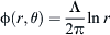 and
and  , where Λ is the volume flow rate from the source per unit length. If the uniform flow and the source flow are combined, a potential flow pattern similar to the one in Fig. 4.1C is obtained. A streamline, ABC, is formed over which the flow cannot cross. A wall can be placed over this streamline and the flow will not be affected. The velocity potential and the stream function of the new flow are the sum of those from the uniform flow and the source flow, i.e.,
 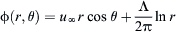 and
and  . These functions can then be used in Eqs. 2.18 and 2.19 to obtain ur and uθ.

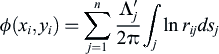
It is, however, not always easy and straightforward to guess the combinations of elementary flows required to model complex flows. Instead the external structure of a complicated geometry, such as a train, is used to obtain the elementary flow around it by dividing the external structure into a number of panels, each panel representing a source sheet (consisting of an infinite number of line sources). Fig. 4.2 represents an example of a two-dimensional cross section of a train subjected to a uniform crosswind of velocity V∞.
Denote  to be the source strength per unit length along s. The small portion of a panel of length ds has a volume flow rate equal to
  . It is assumed that the source strength
  per unit length is constant over a given panel, but it is allowed to vary from one panel to the next. The problem now is to find the known source strength for each panel that gives zero velocity in the normal direction of each panel. Using the superposition principle for the potential flow of number of sources from the panels and the uniform flow, it is straightforward to obtain the velocity potential at the control point of panel i due just to the other sources (i.e., ignoring the free stream crosswind) along the wall to be
 (4.1)
(4.1)where j is the panel number and  .
.
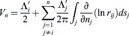
The velocity normal to the panel at panel i is the derivative of the velocity potential in the direction of the normal unit vector n. This gives the normal velocity at the centre of panel i due to the sources at the other panel as
 (4.2)
(4.2)The total normal velocity at panel i is the sum of the normal velocity due to the different sources at the different panels from j to n and the normal velocity due to the uniform free stream velocity. This normal velocity should be zero to satisfy the impermeability boundary condition at the wall of the train. This gives
 (4.3)
(4.3)The angle βi in Eq. (4.3) is the angle between the direction of the uniform flow and the unit normal direction at panel i.
Eq. (4.2) is one equation in n number of unknowns  . Similar equations can be obtained for each panel to create a system of linear equations that can be solved for the source strength at each panel. Once the source strengths are obtained, then the velocity potential and the velocity components can also be obtained. The smaller the panel length, the more accurate the solution will be. It is worth mentioning here that vortex sheets can be used instead of source sheets to account for the vorticity in the boundary layer of the train. If vortex sheets are used, then the method is called the vortex panel method. As this is a two-dimensional method, it can be used for calculating the flow on a train in a crosswind far from the nose (Chiu, 1991). If the nose of the train is to be included, or the wind is acting on the train with an angle other than 90 degrees, then more complex vortex panel methods can be used (Chiu, 1995).
4.3. Reynolds-averaged Navier–Stokes methods
4.3.1. Representation of turbulence
Turbulence is that chaotic state of motion characteristic of high Reynolds number flows. Resolving all the turbulent scales in space and time using DNS (see below) is feasible only for very fundamental and academic problems at very low Reynolds numbers. However, the flow around trains is characterised by high Reynolds numbers, and resolving all turbulent scales is nearly impossible, even on present-day computers. It is worth mentioning that even if computers were able to solve a more complicated flow in an adequate time, there would still be a need to organise by averaging the huge amount of random data to understand the turbulent flow. It is easier to average the governing equations first and then to solve them afterwards. The time-averaged equations are called the RANS equations and are presented in Eqs. (2.7)–(2.9) for two-dimensional incompressible flow. RANS models are very widely used in train aerodynamics to study a range of problems, and these applications will be described in Chapters 7–12. It should be remembered, however, that these are, in general, steady flow methods, and thus where there is large-scale unsteadiness, this will not be captured by RANS calculations. In particular, in large-scale separated flows, the flow patterns will be time-average patterns, which will not fully represent the conditions found at full scale. Nonetheless, the relative simplicity of RANS models and the fact that they can be run on relatively small work stations make them a popular tool despite their acknowledged drawbacks.
From the point of view of the averaged motion at least, the problem with the nonlinearity of the instantaneous equations is that they introduce new unknowns, the Reynolds stresses, into the averaged equations. For three-dimensional flow, there are six individual stress components we must deal with; to be exact:  ,
,  ,
,  ,
,  ,
,  and
and  . The absence of additional equations for these unknowns is often referred to as the turbulence closure problem and it is therefore necessary to model the Reynolds stress terms in some way. There exist mainly two different kinds of turbulence models for this purpose, turbulent viscosity models and Reynolds stress models, and we consider these in turn below (4.3.2 and 4.3.3), before moving on to look briefly at URANS models (4.3.4).
4.3.2. Turbulence viscosity models
The turbulent (or eddy) viscosity models act on the assumption that the Reynolds ‘stresses’ can be expressed in a similar way to the viscous stress term because they also resist the flow motion in some way – the Boussinesq eddy viscosity assumption. This assumption implies that the Reynolds stress tensor is proportional to the mean strain rate tensor. In tensor form, this leads to
k is the kinetic energy, expressed as
and  is the mean strain rate defined by
 (4.7)
(4.7)In Cartesian form, the term  is represented as
 (4.8)
(4.8)The turbulent dynamic eddy viscosity, μt, in Eq. (4.8) has to be modelled. This term is not a property of the fluid, but a feature of the flow and it depends on position and time.
The simplest approach to specifying the turbulent viscosity is to use Prandtl's mixing length model. In this model, the effective viscosity μt is taken as being proportional to the square of a quantity having the dimensions of length, i.e., the so-called mixing length, lmix, multiplied by the absolute value of the local velocity gradient  . Thus
As Eq. (4.9) shows, the mixing length model does not need any extra transport equations to solve for the eddy viscosity and hence this model is called the zero-equation model. The main problem of this model is that there is no universal value for the mixing length and it is very difficult to decide the value for the different types of flows.
Other, more complex, models can be used where the turbulent viscosity is modelled by one or more equations. The most common of these is known as the k − ε model, which is a two-equation model for the eddy viscosity μt. The turbulent viscosity is obtained by using the turbulent kinetic energy k and the rate of dissipation ε. The turbulent kinetic energy is defined as
These variables are determined from transport equations that have the same form for both k and ε and involve convection, diffusion, production and dissipation terms, which involve a number of empirically determined equations. The method effectively assumes that the flow is isotropic, i.e., the turbulence components do not vary with direction. Using dimensional analysis, the expression for the eddy viscosity can be found as follows:
Balancing the dimensions on both sides of Eq. (4.11) yields the following:
where Cμ is the model constant, Cμ = 0.009. The value of this constant has been arrived at by numerous iterations of data fitting for a wide range of turbulent flows.
In addition to the zero-equation model and the two-equation k-ε model, there is a large range of other turbulence models including one-equation models such as the Spalart–Allmaras (S-A) model (see Section 4.4.3 below) and two-equation models such as k-ω and Shear Stress Transport model (SST). Each of these models has advantages and disadvantages. Some of them will work very well to predict the mean flow in certain conditions but fail to predict the flow in another situation. At the present, there is no universal turbulence eddy viscosity model that can accurately predict the mean flow in all kind of engineering problems.
4.3.3. Reynolds stress models
Instead of modelling the turbulence viscosity, Reynolds stress models use the Reynolds stress transport equations to specify the Reynolds stress tensor in the Navier–Stokes equations. This accounts for the directional effects of the Reynolds stresses and the complex turbulent flow interactions. As such, it is often claimed that Reynolds stress models offer significantly better accuracy than isotropic eddy viscosity–based turbulence models. Each of the six transport equations includes terms for transport of Reynolds stress by diffusion, turbulent pressure–strain interactions and rotations, together with production and dissipation terms. Most of these terms require modelling in some way, although these models are at a more detailed and more universal level than the modelling of eddy viscosity in the approaches outlined in the last section.
4.3.4. Unsteady Reynolds-averaged Navier–Stokes
In RANS modelling, the Navier–Stokes equations are time-averaged, and thus the time derivative disappears from the RANS equations. However, if the equations are averaged over a small time, then the time derivative remains in the equations and the variables in the equations represent the mean quantities during the small averaged time. This is called the URANS. The averaging process over the small averaging time produces Reynolds stresses similar to those in the RANS modelling, and the modelling of these stresses is done in the same way as those of the RANS models.
4.4. Direct numerical simulation
4.4.1. Cell size and time step limits
DNS involves the solution of the governing equations of the flow directly, without any assumptions or simplifications to obtain the exact instantaneous motions. In DNS, the number of equations is equal to the number of unknowns (i.e., four equations for four unknowns ux, uy, uz and p). Now, it is a fact that the minimum turbulent eddy size that can be obtained from a numerical simulation is the size of the computational cell, Δ. Thus to resolve all the scales of the flow in DNS, the cell size should be of the order of magnitude of the smallest scale in the flow, which is given by the Kolmogorov dissipation scale lK
where li is the integral length scale and Reli is the Reynolds number based on this scale. Thus the number of cells needed for DNS increases with the Reynolds number. The time step, Δt, required by DNS also has to be very small to resolve the flow in time. There are two factors that control the choice of the time step. It should be smaller than the Kolmogorov time scale, τK, and to maintain numerical stability and accuracy, the time step should also be small enough that the fluid particles do not move more than one grid spacing in each time step. For the one-dimensional flow shown in Fig. 4.3, this implies that
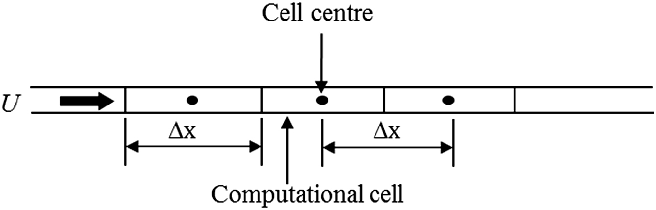
where Δx is the spacing between nodes and U is the velocity.
The left hand side of Eq. (4.14) is called the Courant–Friedrichs–Lewy (CFL) number. To satisfy both limits,  . For high Reynolds numbers, the flow is dominated by very fine structures associated with very small scales, and for any practical flow the total number of cells needed to resolve all the scales is very large, and hence the computational cost is also very high. This means that DNS is not feasible at the present time for solving high Reynolds number flow such as the flow around trains. There are, however, hybrid methods available that use DNS for the large-scale turbulence or for parts of the flow field, and some sort of turbulence modelling for small-scale turbulence and other parts of the flow, and these will be discussed in the following sections.
4.4.2. Large Eddy Simulation
LES decomposes the structures of the flow into large and small scales. The large motions of the flow are directly simulated, while the influence of the small scales on the large-scale motions is modelled. LES thus requires less computational effort than DNS, but more effort than RANS. The main advantage of LES over the computationally cheaper RANS approaches is the increased level of detail it can deliver. While RANS methods provide averaged results, LES is able to predict instantaneous flow characteristics and resolve turbulent flow structures. LES also offers significantly more accurate results than RANS for flows involving flow separation.
Now, Kolmogorov's assumptions about the energy cascade in turbulence flows from large-scale turbulence to small-scale turbulence imply that the small-scale structures behave in a universal way independent of the boundary conditions used. The large flow structure, on the other hand, depends mainly on the boundary conditions and these depend on the problem under consideration. These attributes are the reason why it is useful to model only the small structures and simulate the big ones.
The first step in LES is to filter the equations. The actual velocity,  , is decomposed into a filtered part
  and a subgrid component of velocity
  as
as
The filtered velocity is obtained by filtering the actual velocity as follows:
where the integration is over the entire flow domain, and  is the filter function. The filtered velocity is not the same as the actual velocity field and the difference is the residual .
The equations for the large-scale eddies can be derived through filtering the Navier–Stokes equations. The filtered continuity and momentum equations for two-dimensional incompressible flows are
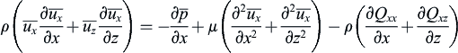 (4.18)
 (4.19)
where Qxx, Qxz, Qzx and Qxz are the residual stresses.
The smallest eddies that can be resolved in any grid are of the size of the grid spacing. However, the flow includes smaller scales than the resolved ones. The residual stresses are a direct consequence of the filtering process and they compensate for the effect of the unresolved or subgrid-scale eddies on the resolved eddies.
The turbulence models for the residual stresses are analogous to the models used for the Reynolds stresses by RANS. It is known that small scales tend to be more homogeneous and universal and less affected by the boundary conditions. Thus their models are simpler and require fewer adjustments when applied to different flows. The simplest formulation is the one-equation model proposed by Smagorinsky. It models the subgrid-scale Reynolds stress analogously to the way this is done in the eddy viscosity models. The anisotropic residual stress tensor, Qij, is related to the filtered rate of strain as  , where vt is the subgrid-scale eddy viscosity, which acts as an artificial viscosity and represents the eddy viscosity of the residual motion. It is modelled as the product of a length scale and velocity scale. According to Smagorinsky, this is modelled as
The length scale in Eq. (4.20) is modelled as  , where Cs is the Smagorinsky coefficient and
  is the filter width.
The computational cost of LES is relatively low compared with that of DNS because all the turbulent scales are not resolved. In LES, the large eddies are solved directly and the influences of the small-scale eddies on the large-scale eddies are modelled. The size of the smallest scale eddy that can be resolved in LES is the size of the cell in the grid. Of course, the computational expense of LES is higher than that of RANS, but it is more accurate for flows in which large-scale unsteadiness is significant, such as the flow around trains. LES has been successfully applied for the flow around trains to obtain the train slipstream and aerodynamic forces (Hemida and Krajnović, 2008a, 2010; Krajnović, 2009b; Hemida and Baker, 2010; Flynn et al., 2014.
4.4.3. Detached Eddy Simulation
In the DES approach, URANS models are employed in the near-wall regions, while the filtered versions of the same models are used in the regions away from the wall, i.e., LES modelling. The LES region is normally associated with the core turbulent region where large turbulence scales play a dominant role. In this region, the DES method uses the LES subgrid models. In the near-wall region, the respective RANS models are used. One of the commonly used turbulent models with DES in the case of external flow is the one-equation S-A model. DES has been recently used intensively for train aerodynamics due to the fact that it is less computationally expensive than LES and provides much better time-averaged results than steady and URANS (Morden et al., 2015, Li et al., 2018a; Flynn et al., 2014).
4.5. Lattice Boltzmann method
LBM is a relatively new form of CFD that has come to be particularly popular in road vehicle aerodynamics in the last two decades. Rather than using the Navier–Stokes equations for a fluid continuum, LBM models the fluid as a large number of particles that are transported over a discrete lattice mesh, and collide with other particles, using the Boltzmann equation for the statistical behaviour of dynamic particle systems. This method can be shown to be equivalent to solutions of the Navier–Stokes equations for incompressible, low Mach number flows. It has effectively been used as a form of LES, with LBM being used to calculate the large-scale turbulence, and turbulence models of various types being used to calculate the small-scale turbulence. Its main advantage is its speed of calculation, as the model has been developed for massive parallel computation. The main disadvantage of this method is the fact that the mesh has to be uniform over the entire flow field and the mesh spacing in the three orthogonal directions needs to be similar. To date, the method has found little application to train aerodynamics, with the only works known to the authors being that of Wang et al. (2008), where it was used to calculate a range of flows around a short high speed train with and without crosswinds, and the work of Mohebbi and Rezvani (2018), where it is used to calculate the crosswind forces on trains behind windbreaks. The former used the method to calculate the large-scale turbulent flows and an embedded RANS model for small-scale flows and thus acted in some ways as the equivalent of LES. Neither paper gives details of the numerical methodology that was used. Notwithstanding this present lack of use, it is likely that this methodology will find more applications in train aerodynamics in the coming years.
4.6. Optimisation methods
4.6.1. Rationale
A train in motion experiences different kinds of aerodynamic forces and moments. It is known that the aerodynamics of train depend on its shape. For instance, as will be shown in Chapter 7, the total aerodynamic drag of a train is the sum on the aerodynamic drag contributions of the different parts of the train including drag from the nose, tail, bogies, intercarriage gaps, pantographs and the skin friction drag. To reduce the overall drag, the shape of these different parts needs to be modified.
The geometrical shape of trains is complex, and many variables can be optimised to enhance its aerodynamic design. Moreover, the flow around the trains is very complex, which makes it difficult to develop accurate and reliable design tools to predict an optimal shape. The design of the different variables has traditionally been based on simplified analytical methods and model tests. Optimisation has been handled in a trial-and-error design procedure that relies on the skills and experience of the aerodynamicist. Optimisation of the aerodynamic properties of trains is always a multi-objective (drag, lift, side force and aerodynamic moments) problem. Moreover, several aerodynamic objectives are known to be in conflict. For instance, reducing the drag of a train by changing its shape often produces high lift or high side forces. A resulting optimum shape should then compromise between these objective functions. There is thus a need for a more systematic approach, capable of identifying and comparing different trade-offs of multiobjective design.
4.6.2. Design approach
Without a clear strategy for a design method, the shape optimisation of one objective variable may require a large number of experiments (computational simulations or wind tunnel tests). This is not feasible and impractical in an engineering sense. Instead, an engineering approach should be used to limit the number of experiments and hence reduce design costs. For multi-objective optimisation, the first step is to define the objective functions (the desired variables or outputs that we need to reduce such as drag force, lift force, side force and rolling moment, for instance). Also, the design variables need to be defined before the optimisation process. If we take the train nose as an example, there is an infinite number of shape designs that can be thought of and this leads to infinite number of experiments required. The most common method to achieve this is to use a surrogate model to estimate responses of the experiments at small sequences of design points for the design variables. The design points chosen for the experiments are not selected randomly but follow a special strategy called design of experiments (DOE).
4.6.3. Design of experiments
The design of experiments (DOE) is a sequence of experiments (using CFD or wind tunnel testing) that will be performed for a number of chosen values of the design variables. There are several design strategies to pick the design values. All of them start by determining the lower bound and upper bound of the design variables and then choose some points in between at which the experiments will be performed. The most common methods of generating these points are the cantered composite design (CCD) method and the optimal Latin hypercube sampling (opt.-LHS) method. In the CCD method, the design points are chosen at the lower and upper bonds and at the centre between them. This means that for two design variables, a minimum of nine design data points is needed. This method has been used by Hemida and Krajnović (2008c) for shape optimisation of a double-decker bus and Krajnović (2008) and Krajnović (2009a) for high-speed trains. The LHS design is constructed in such a way that each one of the design variables is divided into N equal levels and that there is only one point (or experiment) for each level. The final Latin hypercube design then has N design point. The opt.-LHS design augments the Latin hypercube design by requiring that the sample points be distributed as uniformly as possible throughout the design space in an optimum way (Viana et al., 2010). Fig. 4.4A shows a design space using the CCD method for two design variables x1 and x2, while Fig. 4.4B and C shows two possible design spaces for the same design variables using opt.-LHS and five design points. This method has been used for the shape optimisation of high-speed trains by Li et al. (2016), Yao et al. (2014) and Ming et al. (2016).
4.6.4. Surrogate model
Following the DOE, a relationship between the design space and the calculated/measured responses at the design points need to be constructed. This relationship is finally used for obtaining the optimal combination of design variables to fulfil the objectives. The response surface (RS) model is a common method in surrogate model construction. This method is a statistical tool that is useful for modelling and analysis for situations in which the response of interest is a function of several input factors. The RS method has been widely used in practical engineering design optimisation problems, where the optimal searches are based on the RSs mimicking the physical processes or models. It is sometimes the only practical option for performing design optimisation, such as simulation based design optimisation, when simulations are usually computationally expensive. In conventional approaches, the RSs are built up using the group of sampling points based on the DOE scheme. The approximation of the true response in an RS can be represented by low-order polynomials that are normally quadratic. For RS, polynomials are advantageous in that their coefficients can be determined easily using the least square method and in that statistical evaluation can be made of them once their coefficients have been determined. For this reason, function approximations using the least square method are most often used with the RS methodology. For example, for the approximation  of a variable
  , which is a function of
  , one may write

 (4.21)
Representing the above with two variables  and
and  for simplicity gives
Here,  are the model regression coefficients. The error between the approximation value
  and the actual value is
  . Assuming that the number of experiment points is n and the number of design variables is k, the linear regression model can be represented as
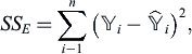
The regression coefficient  can be determined by minimising the sum of the square of the error . A good measure of the fit of the RS with the data is value of the coefficient of multiple determination,
  , which takes the form
Here, SSE is the sum of the squared approximation errors at the n sampling points, SST is the true response's sum of squared variation from the mean and SSR is the approximation's sum of squared variations from the mean, i.e.,
 (4.25)
 (4.26)
 (4.27)
In general, the coefficient of determination, , is used to decide whether a regression model is appropriate. The assessor provides an exact match if it is 1.0, and if the residual increases, decreases in the range from 1.0 to 0. As the number of variables increases, the residual increases so that the determination coefficient increases in value. For this reason, the coefficient of determination adjusted,  , is used to obtain a more precise regression model judgement. takes the form
where k is the number of design variables.
Although a higher value of means a better fit, it is possible that the RS is not the correct representation of the actual data. One way to increase is to increase the degree of the polynomial but it has other consequences. Increasing the degree of the polynomial by more than three results in a large amount of noise in the regression. The backward elimination procedure based on the t statistic is associated with the RS to discard terms and improve the prediction accuracy. The t statistic of the fitted coefficient is defined as its value divided by an estimate of the standard error of the coefficient. In the backward elimination, we begin with the full regression model obtained from the least square method. The t test is performed on all the regression coefficients to determine their influence on the model. A rule of thumb says that regressor terms with an absolute value of larger than 2.0 are significant at a 95% confidence interval. Thus the regressor terms are removed from the model if the regressor's t is smaller than 2.0 and if R2 increases after the regressor's removal. This method has been adapted by Hemida and Krajnović (2008c) and Krajonvić (2009). The method of Kriging explained in Li et al. (2016), Xu et al. (2017) and in Jakubek and Wagner (2016) is also used in shape optimisation for train aerodynamics.
4.6.5. Multi-objective optimisation
The constructed RSs are used an optimisation method to find the multi-objective optimum design. Optimisation methods are generally categorised into two groups: deterministic methods and stochastic ones. Deterministic methods are normally suitable for optimisation processes that only involve only one single peak in the optimisation space. However, if there are multiple peaks in the solution space, then the stochastic methods are more appropriate. In general, the objective functions of the train shape optimisation have plural peaks and thus stochastic methods are the suitable ones.
Among the stochastic approaches, there is an evolutionary algorithm that is widely used for obtaining the optimum shape of high-speed trains. At the beginning of the optimisation process using the evolutionary algorithm, an initial population of design candidates called individuals is randomly generated. Following this initial stage, a fitness function of each individual, which is related to the objective function, is evaluated. Another pair of individuals with higher fitness values is then selected to produce children for the next generation by exchanging and mutating their design parameters. The fitness functions of the new generation are then evaluated and the mating pairs are selected to reproduce the next generation again. As the evolutionary algorithm can sample as many solutions as the number of individuals during the alternation of generations, the Pareto optimal solutions can easily be obtained. The different steps involved in this method are explained in Suzuki and Nakade (2013) and in Deb and Datta (2010).
For shape optimisation of trains using the evolutionary multiobjective optimisation procedure, the so-called real-coded generic algorithm (NSGA-II) developed by Deb (2001) is normally used. The main aim of the algorithm is to find solutions such that there is no other solution for which at least one objective has better value while values of remaining objectives are the same or better.
..................Content has been hidden....................
You can't read the all page of ebook, please click here login for view all page.