Sampling rate changes come in two flavors: rate decreases and rate increases. Decreasing the sampling rate is known as decimation. (The term decimation is somewhat of a misnomer, because decimation originally meant to reduce by a factor of ten. Currently, decimation is the term used for reducing the sample rate by any integer factor.) When the sampling rate is being increased, the process is known as interpolation, i.e., estimating intermediate sample values. Because decimation is the simplest of the two rate changing schemes, let's explore it first.

We can decimate, or downsample, a sequence of sampled values by a factor of D by retaining every Dth sample and discarding the remaining samples. Relative to the original sample rate, f_old, the new sample rate is

Equation 10-1. 

For example, to decimate a sequence x_old(n) by a factor of D = 3, we retain x_old(0) and discard x_old(1) and x_old(2), retain x_old(3) and discard x_old(4) and x_old(5), retain x_old(6), and so on as shown in Figure 10-1. So x_new(n) = x_old(3n), where n = 0, 1, 2, etc. The result of this decimation process is identical to the result of originally sampling at a rate of f_new = f_old/3 to obtain x_new(n).

Figure 10-1. Sample rate conversion: (a) original sequence; (b) decimated by three sequence.

The spectral implications of decimation are what we should expect as shown in Figure 10-2, where the spectrum of an original bandlimited continuous signal is indicated by the solid lines. Figure 10-2(a) shows the discrete replicated spectrum of x_old(n), X_old(m). With x_new(n) = x_old(3n), the discrete spectrum X_new(m) is shown in Figure 10-2(b). Two important features are illustrated in Figure 10-2. First, X_new(m) could have been obtained directly by sampling the original continuous signal at a rate of f_new, as opposed to decimating x_old(n) by a factor of 3. And second, there is of course a limit to the amount of decimation that can be performed relative to the bandwidth of the original signal, B. We must ensure f_new > 2B to prevent aliasing after decimation.

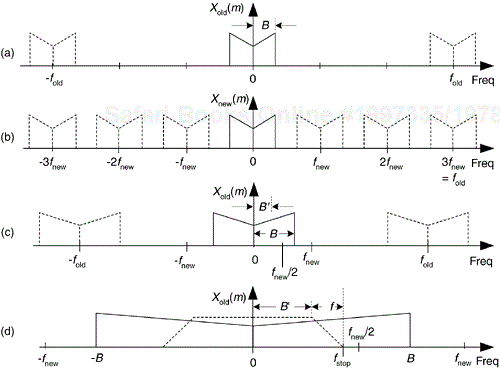
Figure 10-2. Decimation by a factor of three: (a) spectrum of original signal; (b) spectrum after decimation by three; (c) bandwidth B' is to be retained; (d) lowpass filter's cutoff frequency relative to bandwidth B'.

When an application requires f_new to be less than 2B, then x_old(n) must be lowpass filtered before the decimation process is performed, as shown in Figure 10-2(c). If the original signal has a bandwidth B, and we're interested in retaining only the band B', the signal above B' must be lowpass filtered, with full attenuation in the stopband beginning at f_stop, before the decimation process is performed. Figure 10-2(d) shows this in more detail where the frequency response of the lowpass filter, shaded, must attenuate the signal amplitude above B'. In practice, the nonrecursive FIR filter structure in Figure 5-13 is the prevailing choice for decimation filters due to its linear phase response[1].

When the desired decimation factor D is large, say D > 10, there is an important feature of the filter/decimation process to keep in mind. Significant computational savings may be had by implementing decimation in multiple stages as shown in Figure 10-3(a) The decimation (downsampling) operation ↓D₁ means discard all but every D₁th sample. The product of D₁ and D₂ is our desired decimation factor, that is, D₁D₂ = D. The problem is, given a desired total decimation factor D, what should be the values of D₁ and D₂ to minimize the number of taps in lowpass filters LPF₁ and LPF₂? If D = 100, should D₁D₂ be (5)(20), (25)(4), or maybe (10)(10)? Thankfully, thoughtful DSP pioneers answered this question for us[1]. For two-stage filtering and decimation, the optimum value for D₁ is

Equation 10-2. 

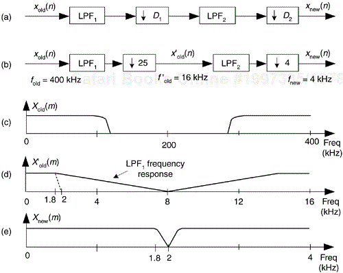
Figure 10-3. Multistage decimation: (a) general decimation block diagram; (b) decimation by 100; (c) spectrum of original signal; (d) output of the D = 25 decimator; (e) output of the D = 4 decimator.

where F is our final transition region width over the stopband frequency, i.e., F = Δf/f_stop. Upon establishing D_1,opt, the second decimation factor is

Equation 10-2'. 

By way of example, let's assume we have input data arriving at a sample rate of 400 kHz, and we must decimate by a factor of D = 100 to obtain a final sample rate of 4 kHz. Also, let's assume the baseband frequency range of interest is from 0 to B' = 1.8 kHz.

So, with f_new = 4 kHz, we must filter out all x_old(n) signal energy above f_new/2 by having our filter transition region be between 1.8 kHz and f_stop = f_new/2 = 2 kHz. Now let's estimate the number of taps, T, required of a single-stage filter/decimate operation. It's been shown that the number of taps T in a standard tapped-delay line FIR lowpass filter is proportional to the ratio of the original sample rate over the filter transition band, Δf in Figure 10-2(d)[1,2]. That is,

Equation 10-3. 

where 2 < k < 3 depending on the desired filter passband ripple and stopband attenuation. So for our case, if k is 2 for example, T = 2(400/0.2) = 4000. Think of it: a FIR filter with 4000 taps (coefficients)! Next let's partition our decimation problem into two stages: with D = 100 and F = (0.2 kHz/2 kHz), Eq. (10-2) yields an optimum D_1,opt decimation factor of 31.9. The closest integer submultiple of 100 to 31.9 is 25, so we set D₁ = 25 and D₂ = 4 as shown in Figure 10-3(b).

We'll assume the original X_old(m) input signal spectrum extends from zero Hz to something greater than 100 kHz, as shown in Figure 10-3(c). If the first lowpass filter LPF₁ has a cutoff frequency of 1.8 kHz and its stopband is defined to begin at 8 kHz, the output of the D = 25 decimator will have the spectrum shown in Figure 10-3(d) where our 1.8 kHz band of interest is shaded. When LPF₂ has a cutoff frequency of 1.8 kHz and f_stop is set equal to f_new/2 = 2 kHz, the output of the D = 4 decimator will have our desired spectrum shown in Figure 10-3(e). The point is, the total number of taps in the two lowpass filters, T_total, is greatly reduced from the 4000 needed by a single filter stage. From Eq. (10-3) for the combined LPF₁ and LPF₂ filters,

Equation 10-4. 

This is an impressive computational savings. Reviewing Eq. (10-3) for each stage, we see in the first stage while f_old = 400 kHz remained constant, we increased Δf. In the second stage, both Δf and f_old were reduced. The fact to remember in Eq. (10-3) is the ratio f_old/Δf has a much more profound effect than k in determining the number of taps necessary in a lowpass filter. This example, although somewhat exaggerated, shows the kind of computational savings afforded by multistage decimation. Isn't it interesting that adding more processing stages to our original D = 100 decimation problem actually decreased the necessary computational requirement?

Just so you'll know, if we'd used D₁ = 50 and D₂ = 2 (or D₁ = 10 and D₂ = 10) in our decimation by 100 example, the total number of filter taps would have been well over 400. Thus D₁ = 25 and D₂ = 4 is the better choice.

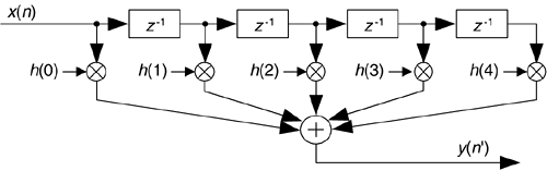
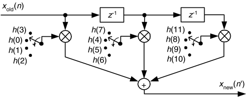
The actual implementation of a filter/decimation process is straightforward. Going back to our original D = 3 decimation example and using the standard tapped-delay line linear-phase FIR filter in Figure 10-4, we compute a y(n') output sample, clock in D = 3 new x(n) samples, and compute the next y(n') output, clock in three new x(n) samples and compute the following y(n') output, and so on. (If our odd-order FIR filter coefficients are symmetrical, such that h(4) = h(0), and h(3) = h(1), there's a clever way to further reduce the number of necessary multiplications, as described in Section 13.7.)

Figure 10-4. Decimation filter implementation.

Before we leave the subject, we mention two unusual aspects of decimation. First, it's interesting that decimation is one of those rare processes that is not time invariant. From the very nature of its operation, we know if we delay the input sequence by one sample, a decimator will generate an entirely different output sequence. For example, if we apply an input sequence x(n) = x(0), x(1), x(2), x(3), x(4), etc., to a decimator and D = 3, the output y(n) will be the sequence x(0), x(3), x(6), etc. Should we delay the input sequence by one sample, our delayed x'(n) input would be x(1), x(2), x(3), x(4), x(5), etc. In this case the decimated output sequence y'(n) would be x(1), x(4), x(7), etc., which is not a delayed version of y(n). Thus a decimator is not time invariant.

Second, decimation does not cause time-domain signal amplitude loss. A sinusoid with a peak-to-peak amplitude of 10 retains this peak-to-peak amplitude after decimation. However, decimation by D does induce a magnitude loss by a factor of D in the frequency domain. Assume the discrete Fourier transform (DFT) of a 300-sample sinusoidal x(n) sequence is |X(m)|. If we decimate x(n) by D = 3 yielding the 100-sample sinusoidal sequence x'(n), the DFT magnitude of x'(n) will be |X'(m)| = |X(m)|/3. This is because DFT magnitudes are proportional to the number of time-domain samples transformed.

To conclude our decimation discussion, a little practical DSP engineering advice is offered here: when we can do so without suffering aliasing errors due to overlapped spectral replications, it's smart to consider decimating our signal sequences whenever possible. Lowering the f_s sample rate of your processing

With that said, think about decimating your signals whenever it's sensible to do so.

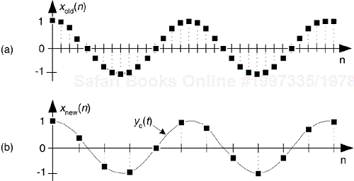
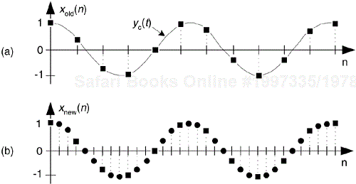
As we said before, decimation is only part of the sample rate conversion story—now let's consider interpolation. Sample rate increase by interpolation is a bit more involved than decimation because with interpolation, new sample values need to be calculated. Conceptually, interpolation comprises the generation of a continuous y_c(t) curve passing through our x_old(n) sampled values, as shown in Figure 10-5(a), followed by sampling that curve at the new sample rate f_new to obtain the interpolated sequence x_new(n) in Figure 10-5(b). Of course, continuous curves can't exist inside a digital machine, so we'll just have to obtain x_new(n) directly from x_old(n). To increase a given sample rate, or upsample, by a factor of M, we have to calculate M-1 intermediate values between each sample in x_old(n). The process is beautifully straightforward and best understood by way of an example.

Figure 10-5. Sample rate conversion: (a) original sequence; (b) interpolated by three sequence.

Let's assume we have the sequence x_old(n), part of which is shown in Figure 10-6(a), and we want to increase its sample rate by a factor of M = 4. The x_old(n) sequence's spectrum is provided in Figure 10-6(a), where the signal spectrum between zero Hz and 4f_old is shown. Please notice: the dashed curves in X_old(m) are spectral replications. To upsample x_old(n) by a factor of four, we typically insert three zeros between each sample, as shown in Figure 10-6(b) to create the new sequence x_int(n'). The 'int' subscript means intermediate. Notice x_int(n') = x_old(n), when n' = 4n. That is, the old sequence is now embedded in the new sequence. The insertion of the zeros (a process called zero stuffing) establishes the sample index for the new sequence x_int(n') where the interpolated values will be assigned.

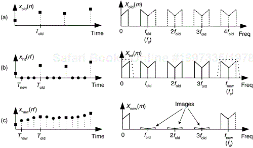
Figure 10-6. Interpolation by a factor of four: (a) original sampled sequence and its spectrum; (b) zeros inserted in original sequence and resulting spectrum; (c) output sequence of interpolation filter and final interpolated spectrum.

The spectrum of x_int(n'), X_int(m), is shown in Figure 10-6(b) where f_new = 4f_old. The solid curves in X_int(m), centered at multiples of f_old, are called images. What we've done by adding the zeros is merely increase the effective sample frequency to f_s = f_new in Figure 10-6(b). The final step in interpolation is to filter the x_int(n') sequence with a lowpass digital filter, whose frequency response is shown as the dashed lines about zero Hz and f_new Hz, in Figure 10-6(b), to attenuate the spectral images. This lowpass filter is called an interpolation filter, and its output sequence is the desired x_new(n') in Figure 10-6(c) having the spectrum X_new(m).

Is that all there is to zero stuffing, interpolation, and filtering? Well, not quite—because we can't implement an ideal lowpass filter, x_new(n') will not be an exact interpolation of x_old(n). The error manifests itself as the residual images within X_new(m). With an ideal filter, these images would not exist. We can only approximate an ideal lowpass interpolation filter. The issue to remember is that the accuracy of our entire interpolation process depends on the stopband attenuation of our lowpass interpolation filter. The lower the attenuation, the more accurate the interpolation. As with decimation, interpolation can be thought of as an exercise in lowpass filter design.

Note that the interpolation process, because of the zero-valued samples, has an inherent amplitude loss factor of M. Thus to achieve unity gain between sequences x_old(n) and x_new(n'), the interpolation filter must have a gain of M.

One last issue regarding interpolation. You might fall into the trap of thinking interpolation was born of modern-day signal processing activities (for example, when we interpolate/upsample a music signal before applying it to a digital-to-analog (D/A) converter for routing to an amplifier and speaker in compact disk players. That upsampling reduces the cost of the analog filter following the D/A converter). Please don't. Ancient astronomical cuneiform tablets (originating in Uruk and Babylon 200 years before the birth of Jesus) indicate linear interpolation was used to fill in the missing tabulated positions of celestial bodies for those times when atmospheric conditions prevented direct observation[3]. Interpolation has been used ever since, for filling in missing data.

Although changing sampling rates, through decimation or interpolation, by integer factors can be useful, what can we do if we need a sample rate change that is not an integer? The good news is we can implement sample rate conversion by any rational fraction M/D with interpolation by an integer factor of M followed by decimation by an integer factor of D. Because the ratio M/D can be obtained as accurately as we want, with the correct choice of integers M and D, we can change sample rates by almost any factor in practice. For example, a sample rate increase by a factor of 7.125 can be performed by an interpolation of M = 57 followed by a decimation of D = 8, because 7.125 = 57/8.

This M/D sample rate change is illustrated as the processes shown in Figure 10-7(a). The upsampling operation ↑M means insert M – 1 zero-valued samples between each x_old(n) sample. The neat part here is that the computational burden of changing the sample rate by the ratio of M/D is less than the sum of an individual interpolation followed by an individual decimation. That's because we can combine the interpolation filter LPF_M and the decimation filter LPF_D into a single filter, shown as LPF_M/D in Figure 10-7(b). The process in Figure 10-7(b) is normally called a sample rate converter because if M > D, we have interpolation, and when D > M, we have decimation. (The filter LPF_M/D is often called a multirate filter.) Filter LPF_M/D must sufficiently attenuate the interpolation spectral images so they don't contaminate our desired signal beyond acceptable limits after decimation.

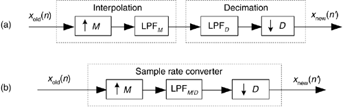
Figure 10-7. Sample rate conversion by a rational factor: (a) combination of interpolation and decimation; (b) sample rate conversion with a single lowpass filter.

Notice that the frequency response of LPF_M/D must be designed so the beginning of its stopband frequency is less than f_new/2 in order to avoid aliasing after the decimation. The stopband attenuation of LPF_M/D must be great enough so the attenuated images do not induce intolerable levels of noise when they're aliased by decimation into the final band of 0 to f_new/2 Hz.

Again, our interpolator/decimator problem is an exercise in lowpass filter design. All the knowledge and tools we have to design lowpass filters can be applied to this task. In software interpolator/decimator design, we want our lowpass filter algorithm to prevent aliasing images and be fast in execution time. For hardware interpolator/decimators, we strive to implement designs optimizing the conflicting goals of high performance (minimum aliasing), simple architecture, high data throughput speed, and low power.

The filtering in sample rate conversion, as we've presented it, is sadly inefficient. Think about interpolating a signal sequence by a factor of 4/3; we'd stuff three zero-valued samples into the original time sequence and apply it to a lowpass filter. Three fourths of the filter multiplication products would be zero. Next we'd discard two thirds of our filter output values. Very inefficient! Fortunately, there are special sample rate conversion filters, called digital polyphase filters, that avoid these inefficiencies. So, let's introduce polyphase filters, and then discuss a special filter, known as a cascaded integrator-comb filter, that's beneficial in hardware sample rate conversion applications.

Let's assume a linear-phase FIR interpolation filter design requires a 12-tap filter; our initial plan is to pass the x_int(n') sequence, Figure 10-8(a), with its zero-valued samples, through the 12-tap FIR filter coefficients shown in Figure 10-8(b), to get the desired x_new(n') sequence. (This filter, whose coefficients are the h(k) sequence, is often called the prototype FIR. That's because later we're going to modify it.) Notice with time advancing to the right in Figure 10-8(a), the filter coefficients are in reversed order, as shown in Figure 10-8(b). This filtering requires 12 multiplications for each x_new(n') output sample, with nine of the products always being zero. As it turns out, we need not perform all 12 multiplications.

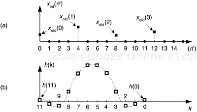
Figure 10-8. Interpolation by four with a 12-tap lowpass FIR filter: (a) filter input samples; (b) filter coefficients, 's, used to compute x_new(n').

To show this by way of an example, returning to our M = 4 interpolation case, let's assume we've decided to use the 12-tap lowpass filter whose coefficients are shown in Figure 10-8(b). The job of our lowpass interpolation filter is to convolve its coefficients with the x_int(n') sequence. Figure 10-9(a) shows the lowpass filter's coefficients being applied to a portion of the x_int(n') samples in order to compute the first sample of x_new(n'), x_new(0). The 12 filter coefficients are indicated by the 's.

Figure 10-9. Filter coefficients used to calculate various x_new(n') samples.

With the dots in Figure 10-9(a) representing the x_int(n') sequence, we see that although there are 12 's and 's, only the three 's generate nonzero products contributing to the convolution sum x_new(0). Those three 's represent FIR filter coefficients h(3), h(7), and h(11). The issue here is we need not perform the multiplications associated with the zero-valued samples in x_int(n'). We only need perform 3 multiplications to get x_new(0). To see the polyphase concept, remember we use the prototype filter coefficients indicated by the 's to compute x_new(0). When we slide the filter's impulse response to the right one sample, we use the coefficients indicated by the circles, in Figure 10-9(b), to calculate x_new(1) because the nonzero values of x_int(n') will line up under the circled coefficients. Those circles represent filter coefficients h(0), h(4), and h(8).

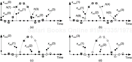
Likewise when we slide the impulse response to the right one more sample to compute x_new(2), we use the coefficients indicated by the diamonds in Figure 10-9(c). Finally, we slide the impulse response to the right once more, and use the coefficients indicated by the triangles in Figure 10-9(d) to compute x_new(3). Sliding the filter's impulse response once more to the right, we would return to using the coefficients indicated by the 's to calculate x_new(4). You can see the pattern here—there are M = 4 different sets of coefficients used to compute x_new(n') from the x_old(n) samples. Each time a new x_new(n') sample value is to be computed, we rotate one step through the four sets of coefficients and calculate as:

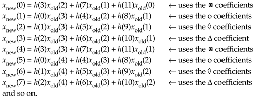
The beautiful parts here are we don't actually have to create the x_int(n') sequence at all, and we perform no unnecessary computations. That is polyphase filtering.

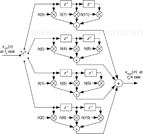
This list of calculations not only shows us what filtering to do, it shows us how to do it. We can implement our polyphase interpolation filtering technique with a bank of four sub-filters as shown in Figure 10-10. This depiction is called the commutator model for polyphase interpolation filters. We have a commutator switch rotating one complete cycle after the arrival of each new x_old(n) sample. This way, four x_new(n') samples are computed for each x_old(n) input sample.

Figure 10-10. Polyphase interpolation-by-four filter structure as a bank of FIR sub-filters.

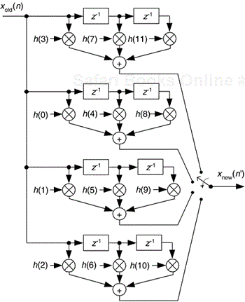
In the general case, if our polyphase filter is interpolating by a factor of M, then we'll have M sub-filters. A minimum-storage structure for the polyphase filter is shown in Figure 10-11, where three commutators rotate (in unison) counterclockwise through four sets of filter coefficients upon the arrival of each new x_old(n) sample. Again, four x_new(n') samples are calculated for each x_old(n) sample.

Figure 10-11. Minimum-storage polyphase filter structure using commutated coefficients.

This scheme has the advantage of reducing the number of storage registers for the x_old(n) input samples. If our polyphase filter is interpolating by a factor of M, then we have M sets of coefficients. We can validate our polyphase FIR filter block diagrams with z-transform equations. We start by describing our polyphase FIR filter with:

Equation 10-5. 

where is a unit delay at the input sample rate, and is a unit delay at the output sample rate implemented with the commutator. Because , and , we can write:

Equation 10-6. 

which is the classic z-domain transfer function for a 12-tap FIR filter. Equation (10-5) is called a polyphase decomposition of Eq. (10-6).

Concerning our Figure 10-9 example, there are several issues to keep in mind:

With the commutating switch structure of Figure 10-10 in mind, we can build a decimation-by-4 polyphase filter using a commutating switch as shown in Figure 10-12. The switch rotates through its four positions (D = 4), applying four x_old(n) input samples to the sub-filters, then the four sub-filters' outputs are accumulated to provide a single x_new(n') output sample. Notice that the sub-filters are unchanged from the interpolation filter in Figure 10-10. The benefit of polyphase decimation filtering means that no unnecessary computations are performed. That is, no computational results are discarded to implement decimation.

Figure 10-12. Polyphase decimation-by-4 filter structure as a bank of FIR sub-filters.

In practice, large changes in sampling rate are accomplished with multiple stages (where Figure 10-12, for example, is a single stage) of cascaded smaller rate change operations of decimation and interpolation. The benefits of cascaded filters are

This introduction to sample rate conversion has, by necessity, only touched the surface of this important signal processing technique. Fortunately for us, the excellent work of early engineers and mathematicians to explore this subject is well documented in the literature.

Several standard DSP textbooks discuss these advanced multirate filter design concepts [5–7], while other texts are devoted exclusively to polyphase filters and multirate processing [8–10]. The inquisitive reader can probe further to learn how to choose the number of stages in a multistage process [1,11], the interrelated considerations of designing optimum FIR filters [1], [12], the benefits of half-band FIR filters [4,13], when IIR filter structures may be advantageous [12], what special considerations are applicable to sample rate conversion in image processing [14–16], guidance in developing the control logic necessary for hardware implementations of rate conversion algorithms [12], how rate conversion improves the usefulness of commercial test equipment [17,18], and software development tools for designing multirate filters[19].

Before concluding the subject of sample rate conversion we'll introduce one final topic, cascaded integrator-comb filters. These filters have become popular for sample rate conversion in the design of modern digital communications systems.

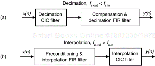
Cascaded integrator-comb (CIC) filters are computationally efficient implementations of narrowband lowpass filters and, as such, are used in conjunction with hardware implementations of decimation and interpolation in modern communications systems.

CIC filters, a special case of the more general frequency sampling filters discussed in Section 7.1, are well-suited for anti-aliasing filtering prior to decimation (sample rate reduction), as shown in Figure 10-13(a); and for anti-imaging filtering for interpolated signals (sample rate increase), as in Figure 10-13(b). Both applications are associated with very high-data rate filtering such as hardware quadrature modulation and demodulation in modern wireless systems, and delta-sigma A/D and D/A converters.

Figure 10-13. CIC filter applications: (a) decimation; (b) interpolation.

Because their frequency magnitude response envelopes are sin(x)/x-like, CIC filters are typically followed, or preceded, by higher performance linear-phase lowpass tapped-delay line FIR filters whose tasks are to compensate for the CIC filter's non-flat passband. That cascaded-filter architecture has valuable benefits. For example, with decimation, narrowband lowpass filtering can be attained at a greatly reduced computational complexity than a single lowpass FIR filter due to the initial CIC filtering. In addition, the follow-on FIR filter operates at reduced clock rates, minimizing power consumption in high-speed hardware applications. An added bonus of using CIC filters is that they require no multiplications.

While CIC filters were introduced to the signal processing community over two decades ago, their application possibilities have grown in recent years[20]. Improvements in VLSI integrated circuit technology, increased use of polyphase filtering techniques, advances in delta-sigma converter implementations, and significant growth in wireless communications systems have spurred much interest in, and improvements upon, traditional CIC filters. Here we'll introduce the structure and behavior of traditional CIC filters, present their frequency-domain performance, and discuss several important implementation issues.

Recursive Running Sum Filter

CIC filters originate with the notion of a recursive running sum filter, which is itself an efficient form of a nonrecursive moving averager. Reviewing the D-point moving average process in Figure 10-14(a), we see D-1 summations (plus one multiply by 1/D) are necessary to compute output y(n).

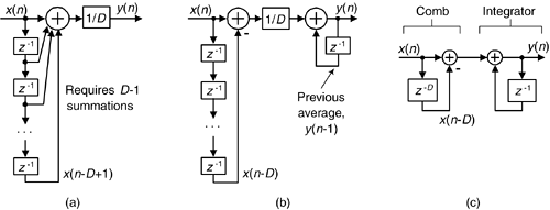
Figure 10-14. D-point averaging filters: (a) standard moving average filter; (b) recursive running sum filter; (c) CIC version of a D-point averaging filter.

The D-tap moving average filter's output in time is expressed as

Equation 10-7. 

The z-domain expression for this moving averager is

Equation 10-8. 

while its z-domain H(z) transfer function is

Equation 10-9. 

An equivalent, but more computationally efficient, form of the moving averager is the recursive running sum filter depicted in Figure 10-14(b), where the current input sample x(n) is added, and the oldest input sample x(n–D) is subtracted from the previous output average y(n–1). The recursive running sum filter's difference equation is

Equation 10-10. 

having a z-domain H(z) transfer function of

Equation 10-11. 

We use the same H(z) variable for the transfer functions of the moving average filter and the recursive running sum filter because their transfer functions are equal to each other. Notice that the moving averager has D-1 delay elements while the initial input delay line of the recursive running sum filter has D delay elements.

The running sum filter has the sweet advantage that only two additions are required per output sample, regardless of the delay length D! This filter is used in many applications seeking noise reduction through averaging. Next we'll see how a CIC filter is itself a recursive running sum filter.

CIC Filter Structures

If we condense the delay line representation and ignore the 1/D scaling in Figure 10-14(b), we obtain the classic form of a first-order CIC filter, whose cascade structure is shown in Figure 10-14(c). The feedforward portion of the CIC filter is called the comb section, whose differential delay is D, while the feedback section is typically called an integrator. The comb stage subtracts a delayed input sample from the current input sample, and the integrator is simply an accumulator to which the next sample is added at each sample period. The CIC filter's difference equation is

Equation 10-12. 

and its z-domain transfer function is

Equation 10-13. 

To see why the CIC filter is of interest, first we examine its time-domain behavior, for D = 5, shown in Figure 10-15. Notice how the positive impulse from the comb filter starts the integrator's all-ones output. Then, D samples later the negative impulse from the comb filter arrives at the integrator to zero all further filter output samples.

Figure 10-15. Single-stage CIC filter time-domain responses when D = 5.

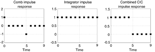
The key issue is the combined unit impulse response of the CIC filter being a rectangular sequence, identical to the unit impulse response of the recursive running sum filter. (Moving averagers, recursive running sum filters, and CIC filters are close kin. They have the same z-domain pole/zero locations, their frequency magnitude responses have identical shapes, their phase responses are identical, and their transfer functions differ only by a constant scale factor.) The frequency magnitude and linear-phase response of a D = 5 CIC filter is shown in Figure 10-16(a), where the frequency axis is normalized to the f_s = f_s,in input signal sample rate.

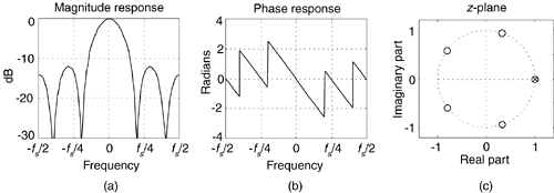
Figure 10-16. Characteristics of a single-stage CIC filter when D = 5: (a) magnitude response; (b) phase response; (c) pole/zero locations.

Evaluating the Eq. 10-13 H_cic(z) transfer function on the unit circle, by setting z = e^jω, yields a CIC filter frequency response of

Equation 10-14. 

Using Euler's identity 2jsin(α) = e^jα – e^–jα, we can write

Equation 10-15. 

resulting in a sin(x)/x-like lowpass filter centered at 0 Hz. (This is why CIC filters are sometimes called sinc filters.) The z-plane pole/zero characteristics of an D = 5 CIC filter are provided in Figure 10-16(c), where the comb filter produces D zeros, equally spaced around the unit-circle, and the integrator produces a single pole canceling the zero at z = 1. Each of the comb's zeros, being an Dth root of 1, are located at z(m) = e^j2πm/D, where m = 0, 1, 2, ..., D-1 corresponding to a magnitude null in Figure 10-16(a).

The normally risky situation of having a filter pole directly on the unit circle need not trouble us here because there is no coefficient quantization error in our H_cic(z) transfer function. CIC filter coefficients are ones and can be represented with perfect precision with fixed-point number formats. Although recursive, CIC filters are guaranteed stable, linear phase, and have finite-length impulse responses.

If we examine just the magnitude of H_cic(e^jω) from Eq. (10-15), we can determine the gain of our single CIC filter at zero Hz. Setting ω in Eq. (10-15) equal to zero, we have

Equation 10-16. 

Don't worry; we can apply the Marquis de L'Hopital's rule to Eq. (10-16), yielding

Equation 10-17. 

So, the DC gain of a CIC filter is equal to the comb filter delay D. This fact will be important to us when we actually implement a CIC filter in hardware.

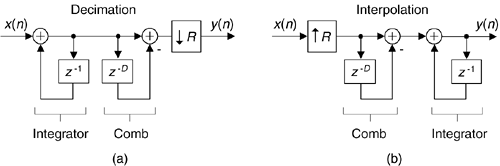
CIC filters are used for anti-aliasing filtering prior to decimation, and for anti-imaging filtering for interpolated signals[21]. With those notions in mind, we swap the order of Figure 10-14(c)'s comb and integrator—we're permitted to do so because those operations are linear—and include decimation by a sample rate change factor R in Figure 10-17(a). (The reader should prove to themselves that the unit impulse response of the integrator/comb combination, prior to the sample rate change, in Figure 10-17(a) is equal to that in Figure 10-15(c).) In most CIC filter applications the rate change R is equal to the comb's differential delay D, but we'll keep them as separate design parameters for now.

Figure 10-17. Single-stage CIC filters, used in: (a) decimation; (b) interpolation.

The decimation operation ↓R means discard all but every Rth sample, resulting in an output sample rate of f_s,out = f_s,in/R. To investigate a CIC filter's frequency-domain behavior in more detail, Figure 10-18(a) shows the frequency magnitude response of a D = 8 CIC filter prior to decimation. The spectral band, of width B, centered at 0 Hz is the desired passband of the filter. A key aspect of CIC filters is the spectral folding that takes place due to decimation.

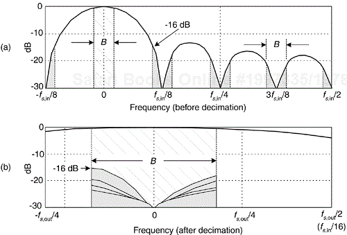
Figure 10-18. Frequency magnitude response of a first-order, D = 8, decimating CIC filter: (a) response before decimation; (b) response and aliasing after R = 8 decimation.

Those B-width shaded spectral bands centered about multiples of f_s,in/R in Figure 10-18(a) will alias directly into our desired passband after decimation by R = 8, as shown in Figure 10-18(b). Notice how the largest aliased spectral component, in this example, is approximately 16 dB below the peak of the band of interest. Of course the aliased power levels depend on the bandwidth B—the smaller B, the less aliasing after decimation.

Figure 10-17(b) shows a CIC filter used for interpolation where the ↑R symbol means insert R-1 zeros between each x(n) sample, yielding a y(n)output sample rate of f_s,out = Rf_s,in. (In this CIC filter discussion, interpolation is defined as zeros-insertion followed by filtering.) Figure 10-19(a) shows an arbitrary baseband spectrum, with its spectral replications, of a signal applied to the D = R = 8 interpolating CIC filter of Figure 10-17(b). The filter's output spectrum in Figure 10-19(b) shows how imperfect filtering gives rise to the undesired spectral images.

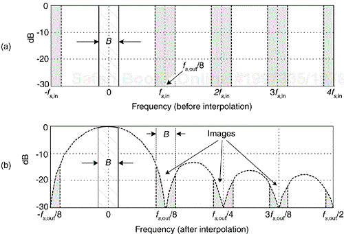
Figure 10-19. First-order, D = R = 8, interpolating CIC filter spectra: (a) input spectrum before interpolation; (b) output spectral images.

After interpolation, unwanted images of the B-width baseband spectrum reside near the null centers, located at integer multiples of f_s,out/R. If we follow the CIC filter with a traditional lowpass tapped-delay line FIR filter, whose stopband includes the first image band, fairly high image rejection can be achieved.

Improving CIC Attenuation

The most common method to improve CIC filter anti-aliasing and image-reject attenuation is by increasing the order M of the CIC filter using multiple stages. Figure 10-20 shows the structure and frequency magnitude response of a third-order (M = 3) CIC decimating filter.

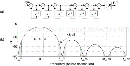
Figure 10-20. Third-order, M = 3, D = R = 8 CIC decimation filter: (a) structure; (b) magnitude response before decimation.

Notice the increased attenuation about f_s,in/R in Figure 10-20(b) compared to the first-order CIC filter in Figure 10-18(a). Because the M = 3 CIC stages are in cascade, the overall frequency magnitude response will be the product of their individual responses, or

Equation 10-18. 

The price we pay for improved anti-alias attenuation is additional hardware adders and increased CIC filter passband droop. An additional penalty of increased orders comes from the gain of the filter, which is exponential with the order. Because CIC filters generally must work with full precision to remain stable, the number of bits in the adders is Mlog₂(D), so there is a large data word-width penalty for higher order filters. Even so, this multistage implementation is common in commercial integrated circuits, where an Mth-order CIC filter is often called a sinc^M filter.

CIC Filter Implementation Issues

In CIC filters, the comb section can precede, or follow, the integrator section. However, it's sensible to put the comb section on the side of the filter operating at the lower sample rate to reduce the storage requirements in the delay. Swapping the Figure 10-17 comb filters with the rate change operations results in the most common implementation of CIC filters, as shown in Figure 10-21. Notice that the decimation filter's comb section now has a delay length (differential delay) of N = D/R. That's because an N-sample delay after decimation by R is equivalent to a D-sample delay before decimation by R. Likewise for the interpolation filter: an N-sample delay before interpolation by R is equivalent to a D-sample delay after interpolation by R.

Figure 10-21. Single-stage CIC filter implementations: (a) for decimation; (b) for interpolation.

Those Figure 10-21 configurations yield two major benefits: first, the comb section's new differential delay is decreased to N = D/R, reducing data storage requirements; second, the comb section now operates at a reduced clock rate. Both of these effects reduce hardware power consumption.

The comb section's differential delay design parameter N is typically 1 or 2 for high sample rate ratios, as often used in up/down-converters. N effectively sets the number of nulls in the frequency response of a decimation filter, as shown in Figure 10-22(a).

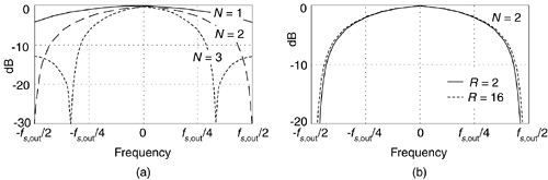
Figure 10-22. CIC decimation filter frequency responses: (a) for various values of differential delay N, when R = 8; (b) for two decimation factors when N = 2.

An important characteristic of a CIC decimator is that the shape of the filter response changes very little, as shown in Figure 10-22(b), as a function of the decimation ratio. For R larger than about 16, the change in the filter shape is negligible. This allows the same compensation FIR filter to be used for variable-decimation ratio systems.

The CIC filter suffers from register overflow because of the unity feedback at each integrator stage. The overflow is of no consequence as long as the following two conditions are met:

1. The range of the number system is greater than or equal to the maximum value expected at the output.

2. The filter is implemented with two's complement (non-saturating) arithmetic.

As shown in Eq. (10-17), a first-order CIC filter has a gain of D = NR at 0 Hz (DC), and M cascaded CIC decimation filters have a net gain of (NR)^M. Each additional integrator must add another NR bits for proper operation. Interpolating CIC filters have zeros inserted between input samples reducing its gain by a factor of 1/R to account for the zero-valued samples, so the net gain of an interpolating CIC filter is (NR)^M/R. Because the filter must use integer arithmetic, the word widths at each stage in the filter must be wide enough to accommodate the maximum signal (full scale input times the gain) at that stage.

Although the gain of a CIC decimation filter is (NR)^M, individual integrators can experience overflow. (Their gain is infinite at DC.) As such, the use of two's complement arithmetic resolves this overflow situation just so long as the integrator word width accommodates the maximum difference between any two successive samples (the difference causes no more than a single overflow). Using the two's complement binary format, with its modular wrap-around property, the follow-on comb filter will properly compute the correct difference between two successive integrator output samples. To illustrate this principle, Figure 10-23 shows how with decimation, using a four-bit two's complement number format, an initial integrator output x_int(0) sample of six is subtracted from a second x_int(1) integrator output sample of 13 (an overflow condition), resulting in a correct difference of plus seven.

Figure 10-23. Two's complement overflow (numerical wrap-around) difference example.

For interpolation, the growth in word size is one bit per comb filter stage; overflow must be avoided for the integrators to accumulate properly. So, we must accommodate an extra bit of data word growth in each comb stage for interpolation. There is some small flexibility in discarding some of the least significant bits (LSBs) within the stages of a CIC filter, at the expense of added noise at the filter's output. The specific effects of this LSB removal are, however, a complicated issue; we refer the reader to Reference [20] for more details.

While this discussion has focused on hard-wired CIC filters, these filters can also be implemented with programmable fixed-point DSP chips. Although those chips have inflexible data paths and fixed word widths, CIC filtering can be advantageous for high sample rate changes. Large word widths can be accommodated with multi-word additions at the expense of extra instructions. Even so, for large sample rate change factors the computational workload per output sample, in fixed-point DSP chips, may be small compared to computations required using a more conventional tapped-delay line FIR filter approach.

Compensation/Preconditioning FIR Filters

In typical decimation/interpolation filtering applications, we desire reasonably flat passband and narrow transition region filter performance. These desirable properties are not provided by CIC filters alone, with their drooping passband gains and wide transition regions. We alleviate this problem, in decimation for example, by following the CIC filter with a compensation nonrecursive FIR filter, as in Figure 10-13(a), to narrow the output bandwidth and flatten the passband gain.

The compensation FIR filter's frequency magnitude response is ideally an inverted version of the CIC filter passband response similar to that shown by the dashed curve in Figure 10-24(a) for a simple three-tap FIR filter whose coefficients are [–1/16, 9/8, –1/16]. With the dotted curve representing the uncompensated passband droop of a first-order R = 8 CIC filter, the solid curve represents the compensated response of the cascaded filters. If either the passband bandwidth or CIC filter order increases, the correction becomes more robust, requiring more compensation FIR filter taps. An example of this situation is shown in Figure 10-24(b), where the dotted curve represents the passband droop of a third-order R = 8 CIC filter and the dashed curve, taking the form of [x/sin(x)]³, is the response of a 15-tap compensation FIR filter having the coefficients [–1, 4, –16, 32, –64, 136, –352, 1312, –352, 136, –64, 32, –16, 4, –1].

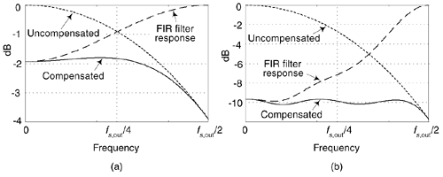
Figure 10-24. Compensation FIR filter magnitude responses: (a) with a first-order decimation CIC filter; (b) with third-order decimation CIC filter.

A wideband correction also means signals near f_s,out/2 are attenuated with the CIC filter and then must be amplified in the correction filter, adding noise. As such, practitioners often limit the passband width of the compensation FIR filter to roughly one-fourth the frequency of the first null in the CIC filter response.^[†]

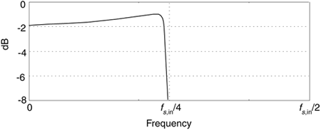
Those dashed curves in Figure 10-24 represent the frequency magnitude responses of compensating FIR filters within which no sample rate change takes place. (The FIR filters' input and output sample rates are equal to the f_s,out output rate of the decimating CIC filter.) If a compensating FIR filter were designed to provide an additional decimation by two, its frequency magnitude response would look similar to that in Figure 10-25, where f_s,in is the compensation filter's input sample rate.

Figure 10-25. Frequency magnitude response of a decimate-by-two compensation FIR filter.

After all of this discussion, just keep in mind: a decimating CIC filter is merely a very efficient recursive implementation of a moving average filter, with NR taps, whose output is decimated by R. Likewise, the interpolating CIC filter is insertion of R-1 zero samples between each input sample followed by an NR tap moving average filter running at the output sample rate f_s,out. The cascade implementations in Figure 10-13 result in total computational workloads far less than using a single FIR filter alone for high sample rate change decimation and interpolation. CIC filter structures are designed to maximize the amount of low sample rate processing to minimize power consumption in high-speed hardware applications. Again, CIC filters require no multiplications, their arithmetic is strictly additions and subtractions. Their performance allows us to state that, technically speaking, CIC filters are lean, mean filtering machines.

Section 13.24 provides a few advanced tricks allowing us to implement nonrecursive CIC filters, and this eases the word width growth problem of the above traditional recursive CIC filters.