CHAPTER 4

Technology Beyond the Standard

In order to better understand the implications of some of the items in the standard, this chapter will provide a bit of additional technical background. The material presented here cannot be considered to be complete, however. The selection of topics is based on many discussions and conversations about MPEG-4 with business-oriented professionals throughout recent years.

4.1. Why Do We Need Compression to Begin With?

Digitizing analog video signals expands physical bandwidth requirements. Physical transmission bandwidth or storage capacity is a natural resource that is scarce and thus expensive. This is where compression of digital data comes into play—to make transmission and storage of digital data economically feasible (Watkinson, 2000a [1], 2000b [2]).

Compression techniques have already been used during the age of analog audio and video as a way to achieve bandwidth reduction and to save cost and natural resources. For example, it takes about 10 times as much data for the digital represtentation of a linear-light progressive scan RGB (Red-Green-Blue) picture, when compared to the representation of the same visual impression as a gamma-corrected interlaced composite video. This fact can also be expressed in that a linear-light progressive scan RGB picture can be represented by the gamma-coded interlaced composite video with a compression factor of 10:1. While the first format is delivered natively by a camera during the course of a movie production, the second is used in television and other forms of entertainment video.

Composite video systems such as the analog domain TV standards PAL, NTSC, and SECAM are all (analog) compression schemes that embed a subcarrier signal, modulated with the color information, in a luminance signal such that color pictures are available in the same bandwidth as monochrome images. Already in the early days of television engineering, it was found that human vision is less sensitive to seeing very fine structures in color signals, i.e., we can see details best in a gray-scale image. This is one reason why color video is represented by color difference signals (YPbPr) instead of plain RGB (Red-Green-Blue). The effect is that the PbPr color difference signals can be presented with a reduced resolution (down-sampled), which lowers bandwidth requirements. Furthermore, the representation of video signals in terms of a gray-level channel (called luma Y) and two color difference signals (called chroma and denoted by PbPr) enabled a backward-compatible migration from black-and-white television to color television in 1953 (NTSC), while preserving the existing channel allocation in the physical frequency spectrum for the TV signals. Thus, consumers could still use their “old” black-and-white TV sets and upgrade to color TV whenever the wanted to. This is a good example of an upgrade policy that treats consumers responsibly.

Gamma correction (non-linear relationship between signal voltage and image brightness) is yet another analog technique to adjust the video signal and the physical characteristics of CRT screens and computer monitors—to better match the characteristics of the human visual perception.

Interlace scan is a widely used technique for signal compression in the analog domain (e.g., NTSC, VHS, etc.). There is a huge amount of legacy video material that is available in this format. The idea of interlacing is to display only one half of an image in one instant of time. This is achieved by showing the odd and the even lines of video images in an alternating sequence. If this alternating display of half images is done quickly enough, human perception is not negatively affected. In fact, interlacing helps to reduce the annoying flicker perception using a higher temporal resolution, while bandwidth is saved. However, in the world of digital video there are more effective ways to compress the video signals. Therefore, interlacing is not really needed any longer as a means for bandwidth reduction or compression. In addition to its being outmoded, dealing with interlaced video generally makes the lives of video engineers more difficult. Most MPEGers would like to get rid of interlaced video material, as do many people dealing with computer graphics and animation. However, there is a massive stock of television and movie content that is stored as interlaced video material, which represents an enormous amount of capital and investment. Thus, interlaced material has become a legacy problem for digital video when the broadcasting industry is the field of application. Today’s TV sets are still dominantly interlaced displays. If the application scenario is either computer-centric, targeting mobile, or handheld terminals, the displays are not interlaced, but are purely “progressive.” (By progressive scan we mean that all lines of one video image are shown at one instance in time.) However, the source material still may be interlaced.

There are several reasons why compression techniques for digital data are popular:

When it comes to compression of audio-visual data, be aware that there are different perceptions of what constitutes a compressed or an uncompressed signal. The attitude toward this question depends on the actual technical environment. A movie producer dealing with Hollywood-quality material filmed on 35mm film or working with high-quality digital production considers a signal that comes in a YCbCr format, using 4:2:0 chroma sampling at a resolution that, according to ITU-T Rec. 601, is a highly compressed signal (never mind the abbreviations). This is in contrast to the point of view of a video-coding expert at MPEG, who calls the very same signal “uncompressed.” A similar point can be made about audio signals. For audio-coding experts, a music signal that comes in stereo with a sample rate of 44.1 kHz with a resolution of 16 linearly quantized bits per sample can be considered an uncompressed signal. This opinion is in direct contrast to the thinking of a professional music recording engineer working in a mastering studio about the very same signal. This difference in the use of terms can lead to some confusion at times.

Let us finish this section with a comment on compression for medical applications. Medical doctors tend to be very critical when it comes to compressing videos and images. They are not willing to accept useful image and video compression technology because there is a chance for the decoded images (images after being compressed and subsequently being decompressed) to slightly deviate from the original images. If the compression technique is applied in an appropriate way, those deviations will not be visible to a human. This is true in particular if the compression is not too hefty. The fact that there may be a mathematical deviation between original and decompressed image is denoted as a lossy compression technology. In contrast to this, a lossless compression technology guarantees the mathematically identical reconstruction of the original image after decompression. In cases where there is a visible deviation between the original image and the decompressed version then those visible deviations are called “coding artifacts.” A lossless coding technology cannot produce artifacts. However, lossy image compression achieves more compression. We will talk about this in more detail later. No physician wants to be sued by some lawyer because he operated on a patient based on a coding artifact introduced by a lossy compression technology. So for medical applications, only lossless compression technology is acceptable, regardless of how lousy the imaging process is that produces the “original” images.

4.1.1. Numerology of Digital Audio-Video Data

Bits and Bytes: Sometimes the use of bits and Bytes can be confusing, especially when actual numbers are at stake. Both terms are commonly used in the context of digital technology. A few remarks on the use of these terms are in order to avoid unnecessary confusion.

The size of a file in the computer world is typically measured in terms of Bytes, where a Byte today is taken to be 8 bits. This is not a globally valid definition for a Byte, but it is the interpretation that most people have come to implicitly agree on. When data is transferred in a computer, for example, from a disk to an external device, the transfer rate is typically measured in Bytes per second.

In a communications environment, engineers measure the number of bits that need to be transmitted from A to B. Therefore, bit rates for transmission are measured in terms of bits per second. As indicated above, there is a factor of 8 between ‘bits per second’ and ‘Bytes per second’, which seems simple enough. Unfortunately, the situation is slightly more complicated. A kilobyte (KB) denotes 2¹⁰ = 1024 Bytes = 1024*8 bits, whereas a kilobit (kbit) = 1000 bits. Similarly, 1 Megabyte (MB) denotes 1024*1024 = 2²⁰ Bytes, and a Megabit (Mbit) is 1000*1000 = 10⁶ bits.

When bit rates for compressed or uncompressed media data are quoted, then the usual measure used is bits/second (bps). Sometimes, in particular when bit rates for video streams over the Internet are quoted, one may read data rates expressed in terms of Bytes per second.

As a general recommendation, we advise reading the quoted numbers carefully with the different meanings in the back of one’s mind.

Image formats and bit rates: The notion of image formats in our context describes the size of the images and the frequency with which the images are displayed as a sequence to generate the impression of moving images. Note that the images are not actually moving. It is a feature of our brain to fuse the fast display of images in order to create the perception of motion in video. Nothing is really moving; it is only pixels that change their brightness and color over time. In that sense, our technical language is somewhat sloppy in referring to moving images, motion estimation, motion in video, and so on. However, it is a useful language that helps to simplify the discussion.

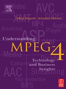
The main impact that actual image formats have in the course of this discussion has to do with the amount of data that the images are creating. In various markets, different image formats are used as input to the video and image encoders. We will cover the more dominant aspects of this topic in order to more easily calculate bit rates even before we start compressing. Table 4.1 lists a number of image formats. The formats differ in the size of the images, starting from the two formats for HDTV, which are the largest, all the way down to QCIF images, which are about 1/8 the size of a regular TV screen. The smaller formats may be used for mobile multimedia.

Table 4.1 Video formats and raw data rates

HDTV typically comes in two sizes. While the United States most commonly relies on the HDTV format with 720x1280 pixels and a frame rate of 60 fps, Europe seems to be more interested in the 1080x1920 format. The formats, according to ITU-T Recommendation 601, come in two versions; one is the 625 version, which corresponds mostly with European PAL systems, and the other is the 525 version, which is associated with the North American NTSC format.

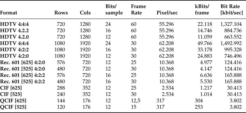
Table 4.2 shows how long video clips can be in order to be storable on either a standard CD-ROM or a standard DVD. (For the purpose of the example, we have assumed that either an HDTV video or a standard definition video clip is being stored.) That is, without compression, it is possible to store 43 seconds of a standard-resolution video on a 650MB CD-ROM. That is a very short movie. Compressing the video using an MPEG-2 video codec at a bit rate of 9 Mbit/sec, we can store a full-resolution video of about 25 minutes in length on a 650MB CD-ROM, and a video of about 74 minutes in length on a 4.7GB DVD. For this example, we have assumed a compression factor of about 13. Typical compression factors for broadcast TV are in the range of 35 or higher. For squeezing the video through an ISDN connection with 64 kbit/sec bandwidth, we require a compression factor in excess of 1900. Clearly, compression is both helpful and necessary.

Table 4.2 Storage of video on disks

Audio resolutions and bit rates: As with video, the main impact that audio formats have concerns the amount of audio data before a compressor starts its work.

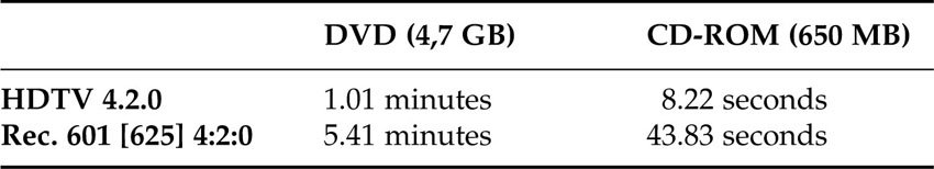
Looking at Table 4.3, one can calculate that a 650MB CD-ROM can store 64 minutes of uncompressed music (consumer CD), while a 64MB flash memory card can only hold stereo music of about 6 minutes in length. An MP3 player with a storage capacity of 64 MB can hold about 69 minutes of music if the material is compressed at a bit rate of 128 kbit/sec. Looking at the fanciest audio format in the table, it is easy to see that audio bit rates are dwarfed by the bit rates necessary for video, which may be one reason audio compression is often underestimated. However, the tremendous success of MP3 makes it clear that high-quality audio compression has a tremendous impact on the music business and the consumer electronics markets.

Table 4.3 Audio formats and uncompressed bit rates

4.2. What Actually Is Compression for Audio-Visual Data?

It is the goal of any type of compression to reduce or minimize the amount of data necessary to represent digitally coded information. Even though the layperson tends to interchange the notions of information and data, a clear distinction is made between the concepts when it comes to compression. Compression is reducing the amount of data while preserving somewhat the information contained in the data.

The data rate of a data source is reduced by the compressor or encoder. The compressed data are then passed through a communication channel or stored on a storage device and returned to the original rate by the decompressor or decoder. The ratio between the source data rate and the channel data rate is called the compression factor. The term “coding gain” is also used. The tandem of an encoder and a decoder is called a codec. Where the encoder is more complex than the decoder, the system is said to be asymmetrical.

Compression of digital data is divided into two major categories—lossless and lossy compression.

4.2.1. Lossless Compression

Lossless compression features a bit-exact reconstruction of data after decompression, i.e., when data is compressed and decompressed, the original data is restored exactly, bit for bit. This implies that there is no loss of information throughout the compression process, which is what a user expects when, for example, he compresses a text file using a ZIP program. After extraction of the corresponding .zip file, the original text file is restored.

The actual compression is achieved by a process that eliminates the redundancy inherent in a given data set. The information content (or entropy) of a sample is a function of how different it is from the value that can be predicted by knowing the value of other samples. Most signals have some degree of predictability. A sine wave is highly predictable, because all cycles look the same. According to Shannon’s theory, any signal that is totally predictable carries no information. In the case of the sine wave, this is clear because it represents a single frequency and so has no bandwidth, and all its values can be safely predicted. The amount of information increases with the unpredictability of an event. The message that the New York Yankees have won the World Series certainly carries less information than the message that the Boston Red Socks finally got rid of the ‘spell of the Babe.’ The second event is clearly harder to predict and may even make bigger headlines. Newspapers have a tendency to measure the amount of information by the size of the printed headlines. An alternative example is the headline “dog bites man” which represents a more predicable or more probable event than “man bites dog.” Therefore, the amount of information carried by the second news item is higher.

At the opposite extreme, a signal such as noise is completely unpredictable and as a result, all codecs find noise difficult or even impossible to compress. The difference between the information rate and the overall bit rate is known as the redundancy. Compression systems are designed to eliminate as much of that redundancy as is practical or perhaps affordable.

The performance of a lossless compression system is measured in terms of compression speed, or computational complexity, for encoding and decoding and the achievable compression factor (calculated as the quotient of the uncompressed file size and the compressed file size) when applied to a set of representative data sets.

Coding performance for lossless compression techniques applied to audio-visual data is typically restricted to compression factors of between 2:1 and 3:1. Lossless compression applied to other types of data, such as text, can lead to significantly higher compression factors. The interested reader may perform some experiments by applying a ZIP program (e.g., WinZIP) to various files sitting on the hard disk. Take for example a Word file, which only contains text, and compress it. Then take a PowerPoint file, which contains text and additional graphical elements or images, and compress this. There should be quite a significant difference in the achieved compression factor.

4.2.2. Lossy Compression

The main difference between lossy and lossless compression is that lossy compression does not allow for a bit-exact reconstruction of the original data after decompression, i.e., the decompressed data deviates from the original data. Therefore, lossy compression is not suitable for compressing computer data such as text files or .exe files.

Lossy codecs are used in situations where the end receiver of the data is a human being. In such a situation, the errors after decoding, that is, the deviation of the decompressed data from the original data, have the property that a human viewer or listener finds them subjectively difficult or even impossible to detect. In other words, the person watching images and listening to audio can not distinguish between the original and the decompressed data. Of course, this statement is conditional to the individual sensory abilities of the person involved. Some people see and hear more than others.

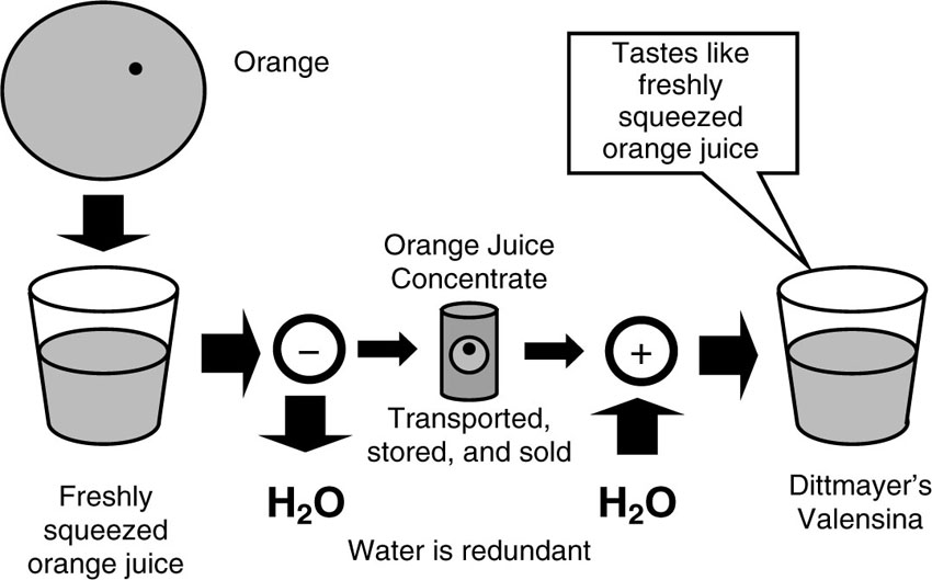
An example of a lossy compression application from everyday life will help to clarify the underlying concepts. For this discussion, consider the illustration in Figure 4.1. Orange Juice is to be produced. Oranges are picked in Florida and squeezed at a factory. If this “freshly squeezed” orange juice is supposed to be shipped around the world, it weighs a lot and the transport would be costly. The producers therefore would want to remove constituents of the juice that are redundant, that is, constituents that are not unique to orange juice from Florida. For example, water is redundant. The formula for pure water is fairly well known around the world (in contrast to the formula for Coca-Cola, for example). Therefore, water can be extracted from the orange juice. This process leaves us with orange juice concentrate, which weighs much less and takes less storage space, and is much easier to package and ship around the world. Once the orange juice arrives at its destination, water can be brought back in to recreate “fresh-squeezed” orange juice. Of course, the orange juice recreated from the concentrate is not identical to the original juice. However, if the process of extracting water, that is, the compression, is done in a faithful way, the recreated juice is hardly distinguishable from the freshly squeezed orange juice. The error is not perceptible, at least for the majority of people. (There will always be some French chefs who can clearly tell the difference.)

Figure 4.1 Schematic representation of the concept of lossy compression.

It’s the same situation with compressing video or audio data. There are always experts with those golden eyes or golden ears who can tell the difference between original and coded data. But the average person will not be able to detect the difference. Lossy compression aims to reduce or eliminate information that is irrelevant to the receiver. If we, as the final receiver of the audio-visual information, cannot hear or see the difference, then it is certainly irrelevant to us.

For a system to eliminate irrelevant information, a good understanding of the psycho-acoustic and the psycho-visual perception process is necessary. Compression systems based on such models or perception are often referred to as perceptive coders. Perceptive coders can be forced to operate at a fixed compression factor. However, in such a situation, the subjective quality of images and audio can vary with the “difficulty” of the corresponding input material.

The performance of a lossy compression technique is measured in terms of the complexity of encoders and decoders as well by assessing the tradeoff between compression factor and quality of the decoded images or audio. Measuring the quality of audio and video compression is a critical and difficult task, which we will discuss in more detail in a later chapter.

Compression factors achieved by lossy compression techniques applied to audio-visual data are generally much higher than the compression achieved by lossless methods, and lies sometimes in the range of 100:1, depending on the application.

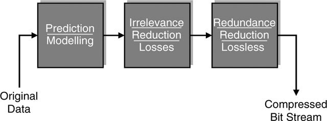
In summary, a data-compression system consists of three major building blocks, which are shown in Figure 4.2. The first box contains algorithms to predict the signal values that are about to be processed. If the system can make good predictions, it understands the signal well and there is not much that needs to be memorized or transmitted in order to recreate the signal. Whatever portion of the signal the predictor cannot predict or anticipate must be unanticipated and hence new information, which will be fed to the second box. In the second box, a mathematical model is included that helps determine which information is supposed to be irrelevant to the receiver. This is the part of the process where data may be lost and the final quality of the audio or video is determined. Finally, whatever is left as relevant information will be further analyzed for inherent redundancies, which can be exploited by a lossless compression algorithm. Thus, the elimination of redundancy in the data sets is also a topic for lossy compression systems.

Figure 4.2 Main building blocks of a lossy compression system for audio-visual data sets.

Of course, a pertaining decoder must invert those processing steps in order to recreate the audio or visual data. However, the information lost in the second block cannot be regained. The lost and (hopefully) irrelevant information is responsible for any type of mathematical deviation between the original signal and the decompressed one. If the model for distinction between relevant and irrelevant information is accurate and precise, a better compression performance can be achieved. This is actually the case with audio coding a` la MP3, where a mathematical model is used to determine the parts of the audio signal which are not perceivable by a human listener, and hence, can be discarded for achieving better compression. The various MP3 encoders in the market mainly differ in the quality of this model for the human hearing system.

In the field of lossy compression, there is no overall theory that helps to precisely predict the achievable compression results of the next-generation lossy compression schemes. The proof of the pudding comes after implementing a coding strategy and assessing the achieved performance by means of subjective tests.

4.2.3. Some Video Coding Terminology

An essential part of MPEG video coding is based on exploiting the similarity of subsequent frames in a video sequence. For a video sequence to make sense for a human the pixels should not change arbitrarily from to frame. If this were the case our brain would not be able to fuse the individual pictures into a continuous flow of moving pictures and the illusion of motion would be lost.

This effect can be used for compression. Subsequent frames of a video sequence have a lot of pixels in common. The pixels are either identical from frame to frame in which case nothing really happens throughout the video. This applies to the background of a scene or if still images are shown. If a picture has been already transmitted and is therefore known to the decoder it is sufficient to only transmitt the pixels that have changed since then in order to update the image. This helps to save bits. If it is not the background then a lot of pixels from the previous frame are still visible in the current frame, but slightly displaced at a different location. This displacement of pixels may be due to moving objects in the sequence. It is not necessary to transmitt all the changed pixels, but it is sufficient to tell the decoder where the pixels have moved in the meantime. This information is conveyed by means of so-called motion vectors, which need to be estimated in the encoder by means of a costly estimation process, the motion estimation.

Based on this concept of only sending information that has changed a compression is achieved for video. In this context three types of images are used, called I-frames, P-frames, and B-frames, which will be introduced in the following.

4.2.3.1. I-Frames

An I-frame is a single frame in a video clip that is compressed without making reference to any previous or subsequent frame in the sequence. This frame is compressed using techniques that are similar to still image compression techniques, such as those employed in the JPEG compression standard. For professional video editing systems that use compression as a means to extend hard disk capacities or required transmission bandwidth, so-called ‘I-frame only’ video codecs are used. This way, a frame-accurate editing of a video clip is still possible. However, using ‘I-frame only’ codecs for video compression is by all means a luxury as such codecs are inferior in compression efficiency as compared to a codec that uses B-frames or P-frames (to be explained in the next sections). For television systems, an I-frame is sent typically every half second in order to enable channel surfing. I-frames are the only frames in a video data stream that can be decoded by its own (i.e., without needing any other frames as reference).

4.2.3.2. P-Frames

P-frames have their name from being predicted from a previous reference frame. That means that if a particular P-frame needs to be decoded, a reference frame is needed which is a frame that appears at an earlier time instant in the sequence (see Figure 4.3).

Figure 4.3 Concept of a P-frame.

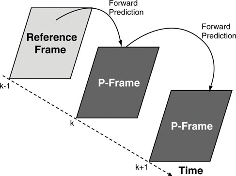
Even though P-frames are based on predictions coming from previous reference frames, a P-frame can again serve as a reference frame for predicting later P-frames. P-frames are an effective video coding tool to improve coding efficiency as compared to a pure image encoder, which compresses each frame individually without making reference to any other frame. All coding schemes offering premium coding performance have a P-frame mechanism employed. However, using P-frames for coding requires the encoder and in the decoder to store the reference frame. A price to be paid for using P-frames is that frame exact editing in the coded bit stream is no longer possible. In order to reconstruct a P-frame the pertaining reference frame is needed. If it is gone due to cutting the video material during editing, the P-frame is gone as well.

4.2.3.3. B-Frames

B-frames have their name from being bi-directionally predicted from at least two reference frames. That means for decoding a particular B-frame a reference frame that appears earlier in the sequence (reference frame 1) and one other reference frame that appears later in the sequence (reference frame 2) are needed (see Figure 4.4).

Figure 4.4 Concept of a B-frame.

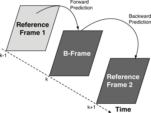
Even though B-frames are based on predictions coming from two neighboring frames, a B-frame is not itself used as a reference frame for predicting other frames. This would lead to an aggregation of coding errors, which kills coding efficiency or image quality. B-frames are an effective video coding tool to improve coding efficiency. All coding schemes offering premium coding performance have a B-frame mechanism employed. However, using B-frames for coding requires more memory in the encoder and in the decoder as an extra frame (reference frame 2) needs to be stored during the decoding process. Furthermore, B-frames introduce extra delay, which is unacceptable for example in conversational applications. There, no B-frames are used. This holds for H.263 and its precursors as well as for MPEG-4 Simple Profile. For television services based on MPEG-2, there are typically 2 successive B-frames between two reference frames to further increase coding efficiency. Another price to be paid by B-frames is that frame exact editing in the coded bit stream is no longer possible. In order to reconstruct the red coloured B-frame in Figure 4.4, both reference frames are needed. If either one of them is gone due to cutting the video material, the B-frame is gone as well.

4.2.4. Constant Bit-Rate Coding (CBR) vs. Variable Bit-Rate Coding (VBR)

CBR coding and VBR coding are two principles that are often mentioned in the context of video coding products. In this section, we give a brief explanation of those modes of operation for a video encoder. For the decoder, both modes are the same as long as the parameters and limitations set by the profiles and level definition are not breached.

Variable bit-rate coding: A compression system as shown in Figure 4.2 produces at its output a bit stream that has a variable bit rate. This variable bit rate is part of the principles employed as a compression algorithm in the encoder. The bit rate variations correspond to the difficulty of the signal to be compressed. In other words, the bit rate increases if the signal carries more relevant information, and it drops if there is very little relevant information in the signal. Hence the name, variable bit rate coding, or VBR for short. The variation in the bit rate is not controlled by any mechanism, and the image or audio quality stays more or less constant, corresponding to “quantization parameter Q,” a coding parameter in the irrelevance reduction block in Figure 4.5, which controls the amount of information that is considered relevant. Therefore, this particular variable bit rate coding mode is more correctly called “constant Q mode.” The bit rate of such an encoder is not predetermined, which is the reason why this mode is hardly ever used in real applications. But for research and development purposes, such as standardization work, this is the regular mode for encoding. One reason why ‘constant Q’ mode is used dominantly during the standardization work is that rate control is a component of the encoding process, which is not the main focus of MPEG standardization. Yet another reason is that in real products, the rate control algorithm is the part that makes the difference in quality between the products of different vendors. This is also the part of the encoder which contains the models for the human perception, to distinguish between relevant and irrelevant information. Thus, rate control is a major aspect of competition. Of course, no serious vendor of MPEG technology is willing to share her own approach or solution for rate control with the competitors during standardization.

Figure 4.5 Rate control for lossy compression system.

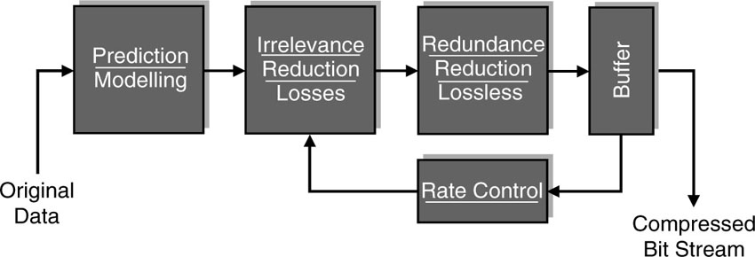
Constant bit-rate coding: An alternative mode of operation, and one that is more standard for an encoder in the market, is to introduce a mechanism to control the bit rate at the output of the encoder. The fullness of a buffer is measured, and according to the level of fullness, a parameter in the irrelevance reduction block is modified in order to influence the production of bits at the output. It is the purpose of the buffer to average out over time the fluctuation of the bit rate. The bit stream is read from the buffer at a constant rate, while it is filled at a variable rate. This works fine as long as the average filling rate is equal to the constant emptying rate. The corresponding encoder structure is shown in Figure 4.5. The result is that the encoder produces a bit stream at its output that has a constant bit rate. Hence the name, constant bit rate or CBR coding.

CBR coding is used when TV channels are distributed over satellite channels, for example. A fixed bandwidth or bit rate is assigned to a TV channel, say 6 Mbit/sec, and charged accordingly. CBR coding is also important when streaming video over the Internet, especially if the users are using connections with a fixed maximum bit rate, like ISDN or dial-up connections. The video needs to be compressed such that the best possible video quality is delivered. To this end, the encoder makes use of the maximum available bit rate. But the maximum coded bit rate must not exceed the transmission capacity, otherwise information may get lost and the video stops or goes black.

Variable bit-rate coding revisited: Let’s come back to variable bit-rate coding for a minute. As mentioned before, a variable bit rate is created by running an encoder with no rate control. But there is another way of creating a bit stream with a variable bit rate. This is done by controlling the bit rate as in the CBR coding scenario (Figure 4.5), but the rate control mechanism tries to adjust the bit rate to achieve a pre-specified average while not exceeding a pre-specified maximum bit rate. This may be seen as the true variable bit-rate coding setup. The benefit over the previously described VBR coding scheme is that the variation of the bit rate is not happening in a random and thus unpredictable way, but under the regime of a rate control algorithm. If the variation in the bit rate is controlled and therefore known, this can be used constructively by broadcasters, for example, to employ statistical multiplexing. Statistical multiplexing is a technique that enables multiple independent TV channels to be transmitted over a satellite link sharing a bulk of bandwidth. Each channel may come as a variable bit-rate stream, and the multiplexer assigns his bandwidth budgets dynamically to the individual channels. This allows savings on bandwidth and cost, somewhere in the range of 20%. However, it may be difficult to guarantee a specific quality of service for the individual channels. From a business point of view, this may make it challenging for the satellite service provider issuing the invoices.

4.3. Do We Still Need Compression in the Future?

Ubiquitous broadband access in the future: As has been widely discussed in press articles, there is a bright future ahead of us, where more and more bandwidth is available for delivering any sort of media data over a variety of transmission channels to any consumer, wherever she is. The list of transmission media includes the Internet (IP networks) and more traditional broadcast channels such as satellite, cable, or terrestrial distribution channels. Various flavors of DSL or cable networks also offer increasing transmission capacities contributing their share to this enjoyable future. Furthermore, wireless technologies such as WLAN, GPRS, or UMTS show the promise of adding further broadband capabilities to the bag of tricks. Regardless of which technology you choose, it is clear that, in the foreseeable future, broadband access will be ubiquitous and affordable for everyone.

Compression technology—dinosaur technology? Imagine a lively discussion between a compression technologist and technology-savvy business person about the long-term value of compression technology. In the course of the discussion, the compression technologist may be faced with the question of why we continue to bother to compress audio-visual data if there is enough bandwidth around to stream or broadcast or exchange any sort of media material. Isn’t media compression about to become the dinosaur of information technology, bound to be extinct once ubiquitous broadband access has arrived?

We could pull out many facts to prove the opposite, to make a strong statement in favor of the longevity of compression technology and to establish it as one of the crown jewels of information technology. Rather than giving such a formal explanation, we’ll draw on a simple story to make the point.

Electrical power generation and consumption 100 years ago: Consider the situation with electrical power at the beginning of the 20th century. While it was technologically possible at that time to produce electrical power, building a large-scale power plant was a technological challenge and not economically feasible. At that time, production and consumption of electrical energy was in its infancy, and the volumes were rather low compared to today. Imagine that there was an entrepreneur who wanted to build a large and modern factory utilizing the latest technology. The factory would contain a large number of machines, all powered by electrical energy. Asking a power production company around 1900 to provide an outlet to offer a couple of hundred Megawatt hours of electrical energy would have represented a major technological challenge and an insurmountable economic obstacle.

Today it still pays to save on electrical power: Today, providing the necessary amount of electrical energy for such a factory no longer poses any real technical or economic challenge. The power company would only ask how much energy is needed and when it should start delivering. In addition, the company would negotiate a price and ask a few questions concerning finances. This last bit of information is still required, as power doesn’t come for free. Today, energy consumption is of course much higher than what people used 100 years ago. But there is also far more electrical power available, and as the price for power drops, more and more appliances are being used that consume electrical power. Power outlets are ubiquitous and electrical power is always available (except for California and some developing countries). However, since energy still costs money, it usually pays to save energy, for example, by using energy-saving light bulbs or dishwashers with an economy mode, and so on. Companies often advise their employees to switch off electrical devices at the end of the day in order to save energy.

Even ubiquitous bandwidth will not be free: Compare this picture of power consumption today to the situation concerning broadband access today and tomorrow. If broadband access is widely available, getting high-speed data connections will no longer be an issue of technological feasibility. Also, as more and more bandwidth becomes available at lower and lower prices, we will be using more and more bandwidth. As a consequence, there will be more and more appliances in use, which will rely on seamless access to broadband data pipes. Finally, transmission or storage bandwidth will become cheaper as time progresses. However, bandwidth will not be completely free, and hence it will still pay to save on bandwidth for the simple reason of cutting cost. Compression is the technology to save bandwidth and thus to save cost. Saving money never seems to be out of fashion.

Ride the wave with largest growth: As a last comment on this topic, observe that the performance of compression is largely dependent on the available computation power. This also means that there is a connection between achievable compression and Moore’s law, which governs the speed by which computing power is increased. Typically, processor performance grows faster than transmission bandwidth. Therefore, it will be more economical to apply compression to digital data as a means to reduce the amount of data than waiting for the next generation of broadband access offering more bandwidth and/or lower prices. To this end, you will need to compare the cost of compression technology with the cost of transmission/storage media.

4.4. Measuring Coding Performance—Science, Marketing, or a Black Art?

Assessing the performance of audio-visual compression technology is done by calculating compression factors and comparing the resulting figures. Also, you may read press releases of companies who make bold statements that their most recent coding product is 10% better than the best previously known codec. While this sounds like a fair enough statement, it is quite difficult to come up with such a conclusion, as it is very difficult to actually quantify such improvements. It is often not clear what aspect of the codec has been improved by those 10%, and what are the conditions under which this claim needs to be seen. That’s all part of marketing and some level of murky statements helps to sell. Therefore, in this section we try to elaborate a bit more on how the quality or performance of audio-visual codecs can be thoroughly assessed. This process may appear to be straightforward at the outset, but the job of testing can involve a number of pitfalls.

4.4.1. Questions on Coding Performance

First of all, for lossy compression of audio-visual data, there is no theory that gives you a formula to determine the coding performance. The performance needs to be evaluated based on coding experiments that are designed to give answers to questions, such as the following.

Besides these questions, there are others that are frequently discussed in public mailing lists, press articles, conferences and the like, the meaning of which sometimes is a bit difficult to understand. Here are some examples.

4.4.2. Calculating a Compression Factor

Out of the many figures of merit, the compression factor achieved by any compression technology is certainly the most interesting single factor to express the performance of a scheme, reminiscent of the use of the clock cycles for expressing the speed of a microprocessor. It is not wrong to state that a computer with double the clock frequency offers more speed and performance than a computer with a lower clock frequency. But experience tells you that the actual performance of a computer system depends on more parameters and characteristics than clock frequency alone.

Compression factor is an easy-to-calculate quantity and a feature that is even easier to sell. So it runs the risk of sometimes being oversold. To calculate the compression, determine the file size or bit rate of the uncompressed material. Next, determine the file size or bit rate of the data after compression. Calculate the quotient of uncompressed and compressed file sizes and—voila—you are done! When comparing the compression performance of two competing systems or schemes, we may face the question of what happens if video parameters are very different and the compression ratios are hard to compare. As we mentioned earlier, there may be different points of view when it comes to the notion of uncompressed material. Starting from HDTV (720p, 60fps) material and compressing it to QCIF resolution at 10fps yields a different compression factor than compressing an NTSC resolution video to CIF resolution at 30fps. In order to compare coding systems operating on entirely different video material, it is helpful to calculate the bit rate in terms of bits/pixels to get a rough idea of coding efficiency, bit rates, and quality.

Let’s look at a small example. We take two video sequences denoted by S₁ and S₂, which have different technical parameters and playing time. The parameters for both sequences are listed in Table 4.4.

Table 4.4 Parameters for the two different test sequences

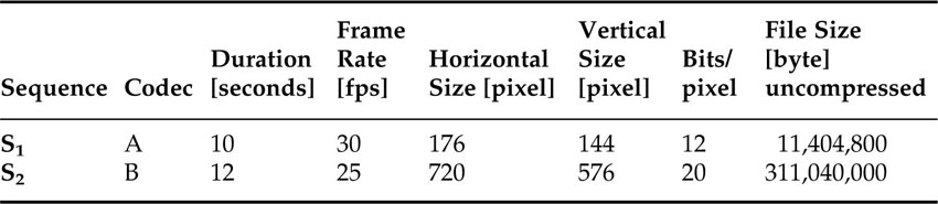
To continue with the same example, we have two codecs denoted by Codec A and Codec B. Sequence S₁ will be encoded with Codec A, and S₂ will be encoded using Codec B. The resulting file sizes for the compressed video sequences are given in Table 4.5 below. Calculating the compression factor based on those file sizes gives the impression that Codec B compresses better than Codec A since it results in a higher compression factor. It needs to be noticed that the two examples S₁ and S₂ are very different in terms of image size and frame rate, for example. In order to take those differences into account it is easy to calculate the average number of bits per pixel. Then it becomes apparent that Codec A and Codec B actually give the same coding performance.

Table 4.5 Parameters for the two different test sequences

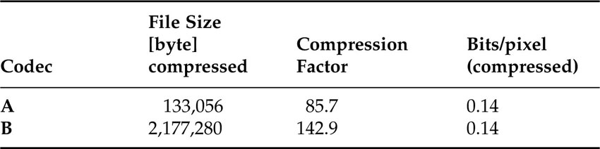
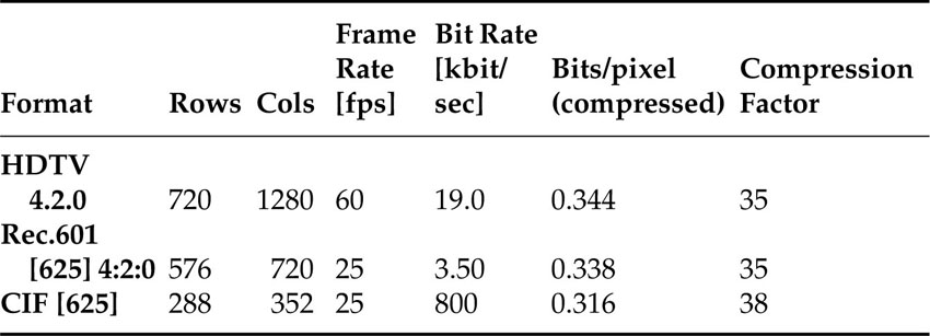
Table 4.6 shows three examples for bit rates that may be used for video services. HDTV television services may operate using bit rates somewhere around 19 Mbit/sec. For standard television services, 3.5 Mbit/sec is not uncommon. Finally, for services over DSL lines, a bit rate of 800 kbit/sec is reasonable. For each of these services, the image size has been reduced to make the video fit the size of the transmission pipes. The bit/pixel calculation for the compressed bit streams for the three services mentioned here show that the compression factor a video codec must provide is in the range of 35.

Table 4.6 Compression factors for three reference applications

Note that the calculation so far implicitly assumes that the visual quality generated by the codecs to be compared is the same. This is generally very difficult to achieve and even more difficult to guarantee. When lossy compression is used, we need to take into account the visual impairments in the compressed video.

This approach of calculating compression factors works well as long as lossless compression is employed exclusively. But if the compression introduces losses, then the compression factors are contingent on the distortion (amount of losses) the audio-visual has endured. There are two basic approaches to doing this.

Approach 1 is the most appealing from a marketing and sales perspective since the final message is easy to quantify and easy to communicate to people. If one particular codec produces 10% better compression, for example, this is easy to communicate and business benefits based on this improvement are easy to calculate. The difficulty with this approach lies in the task of adjusting the parameters for equal visual quality. What does equal visual quality mean and how do you measure it, not to mention shoot for a certain level of quality? In short, this may be a highly desirable way of comparing codecs, but practically speaking, it will not work. If you try to convince a video coding expert to do this type of test, you will immediately see an unhappy face.

Approach 2 is technically the only feasible and sound approach. The difficult part is still the measurement of visual quality, but this can be taken care of by the methodology that is used to design the experiments to be done and the type of measurements to be taken. We will further discuss the quality measurement issue in the section that follows.

4.4.3. Measuring Quality

As mentioned in the previous section, measuring the quality of the compressed video or audio is an essential part of determining the compression performance of a codec. In this section, we will elaborate a bit more on how to measure quality.

All the following explanations are based on the assumption that Approach 2 from the previous section is used. This means that test material is selected (audio or video examples), coding conditions are set, and target bit rates are specified for each test sequence. The encoders compress the test material to produce coded representations of the video or audio samples. Subsequently, the coded bit streams are decoded to create the decompressed video or audio, the quality of which needs to be determined. Quality in this context can be measured fundamentally by two different methods.

Objective measurements: As a unit of quality measurement, the root mean square error is calculated (RMS). The original audio/video signals are taken and the decoded versions are subtracted from them. The result is either an error image or an error sound. All error image pixel values are squared and summed up. The lower the RMS, the better the quality. Engineers often prefer to deal with logarithmic quantities for pure convenience, and therefore the RMS value is transformed into a logarithmic value, which is called PSNR (Peak Signal-to-Noise Ratio). A higher value for the PSNR implies a better quality image. If a quality measure is required for the entire sequence, then the PSNR values for all the frames in the sequence are averaged to produce one single number. The same procedure is applied in principle for audio signals. Interestingly, it has become common for sequence quality measurements to be calculated using the mean value over the PSNR values for all frames, which is mathematically different than calculating the average of the RMS values and then transforming the resulting mean RMS into PSNR. (The second way is the mathematically correct way of doing it.)

This a simple calculation and leads to consistent results. However, the PSNR values do not necessarily correspond very well with the visual quality that is perceived when people are actually looking at the images or listening to the audio. It often happens that in spite of a higher PSNR value, a sequence is visually judged to be inferior. Similarly, it just as often happens that a video sequence shows a lower PSNR value while still being judged to be superior. The same observation holds for assessing audio quality. PSNR is a mathematical tool that does not reflect human visual or audio perception very well, but which is often used due to its simplicity.

Using PSNR values to evaluate visual quality is a reasonable way of answering the second question that was formulated in the previous section. That is, during development of encoders, the progress can be efficiently measured using PSNR.

Unfortunately, in situations where comparisons are to be made between fundamentally different coding techniques, PSNR values become almost useless. This is because if coding techniques are fundamentally different, then they are likely to produce different types of artifacts and the distortions will look or sound very different. In such situations, PSNR does not tell you very much and what it tells you is usually inaccurate. One important method of assessing coding performance involves producing a so-called “rate-distortion curve.” Video codecs typically have a parameter, mentioned earlier, which is called quantization parameter Q. This parameter determines the amount of losses or distortion that a codec produces. Parameter Q has a certain range of permissible values, typically in the range of 1 to 32. In order to determine the rate-distortion curve, a video sequence is coded with all codecs that need to be compared. For each encoding run, a new fixed value for quantization parameter Q is set. This is called “constant Q” coding mode. After the encoding is done, the mean PSNR value for the coded sequence is determined along with the average bit rate (file size divided by length of sequence). Both values are entered in a chart the plots the PSNR values as a function of the average bit rate. An example of such a rate-distortion plot is shown in Figure 4.6.

Figure 4.6 Rate-distortion curve for three different video codecs using constant Q coding mode and measuring PSNR as a measure of quality.

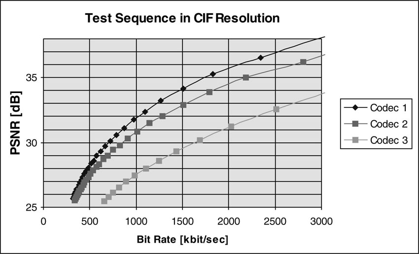
This is a reasonably sound approach for assessing the coding performance of codecs that are not too different in terms of coding techniques. The rate-distortion curve depicted in Figure 4.6 suggests that Codec 3 has only half the coding performance of Codec 2, (i.e., Codec 3 needs about twice the amount of data compared to Codec 2 to achieve the same level of quality). Codec 2 has a PSNR-measured quality of 31 dB at a bit rate of 1 Mbit/sec. Codec 3 requires a bit rate of 2 Mbit/sec to reach the 31 dB point. This observation indicates a 2:1 performance ratio.

Of course, when the rate-distortion curves of many sequences have been determined, then all the corresponding curves can be averaged again to come up with a summarized rate-distortion curve. All of the calculated numbers are easy to plot out and to publish. However, care must be taken not to draw the wrong conclusions from these curves, as they only loosely correspond to subjectively perceived video and audio quality.

Note that there is a lot of averaging going on here. That means that the actual benefits for one codec or another may differ significantly depending on the test material chosen.

Subjective testing: Since measuring compression performance is difficult and it is apparently much easier to issue bold performance claims for any given technology or product, we would like to discuss the subjective assessment of coding quality and performance in some depth. In essence, a thorough performance assessment requires that a subjective evaluation procedure be performed. To do this, people are put in front of a monitor where they watch images and listen to audio and are then asked to vote on what they saw and heard in a kind of blindfolded test. This way, the test subjects rank the codecs based on their subjective quality perception.

There are standards and recommendations for how the experimental setup is supposed to look—what type of monitor, the amount and type of ambient light, the color on the walls of the laboratory environment, the view distance, the voting procedure, and so on. The idea is to be able to create reproducible test conditions in any laboratory around the world and to minimize the influence of the laboratory setup. Another necessary step to ensure the success of the test is to measure the people’s visual acuity to exclude blind or nearly blind test persons. Finally, the choice of tools and techniques for doing the statistical analysis on the voting data is another important task. Detection and removal of outliers and other undesirable trends, as well as the validation of the results, are time-consuming jobs that require experienced and skillful engineers.

All this subjective testing is made necessary by the lossy nature of audio-visual compression technology, and it is the reason why the quality assessment of coding performance for lossy compression systems is a very difficult and costly procedure. Clearly, doing an objective measurement instead would be much easier.

The machinery is available to do such subjective meaningful measurements automatically without the inclusion of test persons, based on the concept of “just noticeable differences” (JND). However, those “objective measurements” are not yet able to provide the full truth—so far the coding experts only rely on real eyeballs if a final conclusion on coding quality is needed.

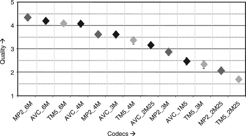
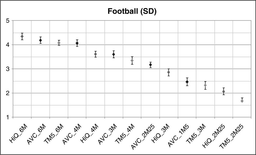
Figure 4.7 is an example of plotted data as it comes out of a subjective test. In this particular test, three codecs (MPEG-4 AVC/H.264, MPEG-2 TM5, and MPEG-2 High Quality) have been tested to compress a sequence called “Football.” The sequence had standard-definition resolution (SD) and was coded with five different bit rates (6, 4, 3, 2.25, and 1 Mbit/sec). The dots in the plot represent the average score the test persons gave, and an error bar is given to indicate the variation of the answers of the test persons. The value 5 represents excellent quality, whereas a value of 1 represents poor quality. A simple but reliable reading of this plot is based on the rule that if the error bars belonging to measurement points have an overlap, then the difference between the average scores are not statistically significant. This particular plot tells us that in this test, AVC at 4 Mbit/sec performed as well as the MPEG-2 High Quality codec at 6 Mbit/sec. Alternatively, one may interpret that AVC at 1 Mbit/sec is visually equivalent to MPEG-2 TM5 at 3 Mbit/sec. Now you can calculate the difference in coding performance and be sure that this is a sound result. However, this result is only valid for the one test sequence. For a more general statement a variety of test sequences need to be coded and voted on.

Figure 4.7 Example of a result from subjective testing of three different codecs (MPEG-4 AVC, MPEG-2 TM5, and MPEG-2 High Quality) on standard-definition resolution video material (“Football” sequence).

In Figure 4.8, another example is shown of a plot from a subjective test. In this particular test, two codecs (MPEG-4 AVC/H.264 and MPEG-4 Advanced Simple Profile) have been tested to compress a sequence called “Mobile and Calendar.” The sequence had a CIF resolution and was coded with four different bit rates (96, 192, 384, and 768 kbit/sec). The dots in the plot represent the average score the test persons gave and an error bar is given to indicate the variation of the test persons’ answers. This plot tells us that in this test, AVC at 192 kbit/sec performs as well as the MPEG-4 ASP codec at 768 kbit/sec. Now you can calculate the difference in coding performance for this case. When the tests are performed using any other set of test sequences, the differences between AVC/H.264 and ASP need not be as pronounced, but will be still significant.

Figure 4.8 Example of a result from subjective testing of two different codecs (MPEG-4 AVC and MPEG-4 Advanced Simple Profile) on CIF resolution video material.

In Figure 4.9, test results are shown for coding a high-definition sequence with an MPEG-4 AVC/H.264 codec, an MPEG-2 High Quality codec, and the MPEG-2 TM4 reference implementation.

Figure 4.9 Example of a result from subjective testing of three different codecs (MPEG-4 AVC, MPEG-2 TM5, and MPEG-2 High Quality) on HD resolution video material at two bit rate s (10 and 20 Mbit/sec). The interested reader is invited to surf the official MPEG Web site (www.chiariglione.org/mpeg), where a number of results on formal tests for earlier standards activities can be found and downloaded.

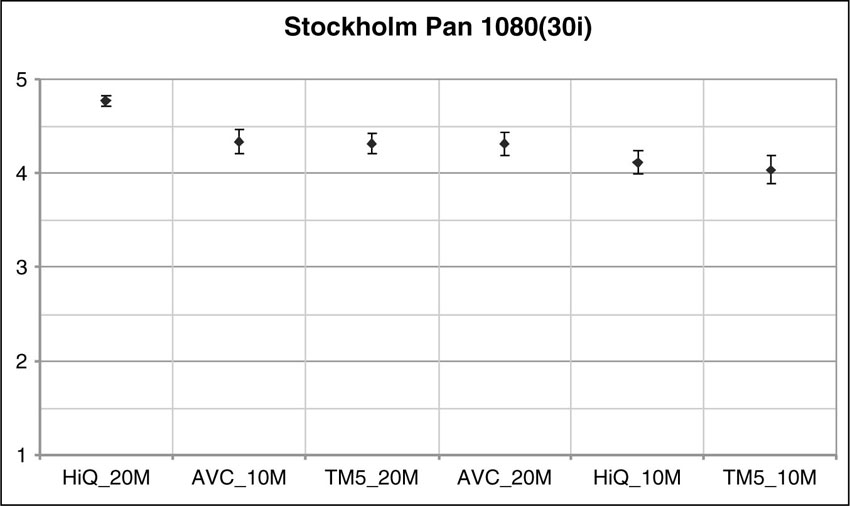
This plot doesn’t make any clear statement about the benefits of coding technologies. One conclusion could be that there is no clearly superior coding technology for this particular example. Another interpretation is that the test material was not sufficiently difficult to encode so that 10 Mbit/sec turned out to be a high enough bit rate to achieve excellent results for all tested codecs.

The choice of test sequences is certainly another important dimension for creating meaningful test results.

4.4.4. Some Notes on Test Material

Testing coding performance is dependent on the availability of good test material. During the development of coding technology, test material must also be produced. It is not always easy to determine what constitutes a good test sequence. Throughout the years, a couple of test sequences have been established as good test material, and these are regularly used. One of the problems with these test sequences is that they are used for development and for testing. This runs the risk of codecs being developed to match the characteristics of the test material used during the development phase. If the same sequences are used for testing and evaluating coding performance, one can expect that the codecs will do fairly well. In principle, the test set should be completely different from the development set. However, there is not much choice for commonly shared and accepted test material.

Another issue with test material has to do with copyright problems. A video has copyrights, and sometimes the sequences cannot be cleared of copyright issues, either because the copyright holder does not agree to grant licenses or because the copyright owner is unknown. Both scenarios lead to a situation of legal uncertainty for all companies involved in standardization. This legal uncertainty prevents the development of a generally accessible and freely usable suite of test sequences that can serve as a common test set for all parties involved in standardization related areas. A number of commercial entities have recently attempted to mend this situation (see Videatis GmbH at www.videatis.com [3] and Video Quality Experts Group [VQEG] at www.vqeg.org [4]).

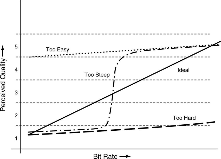
As we have seen in Figure 4.9, sequences may not be sufficiently appropriate to make a clear distinction between a good codec and a worse codec, i.e., the material is such that all codecs either can handle the video content equally well or equally bad. This makes it difficult to make a decision between good and better codecs. In Figure 4.10, test sequences are differentiated as being too easy, or too difficult, or too steep. The figure also shows how the ideal test sequence might look. The curves show the subjective quality perception as a function of bit rate. If the test material is too easy, then there is no clear distinction between different bit rates and it is difficult to assess quality differences. The same holds if the material is too difficult. Then the bit rates are never enough to achieve a good coding result. Too easy and too difficult sequences can also be seen as the upper or lower part of a curve that is too steep. The ideal curve shows a linear relation between bit rate and perceived quality. It is hard to say from looking at a sequence if it is appropriate for testing. Only testing will reveal that. That is why test sequences that have been found over time to fulfill the requirement of creating a smooth transition curve, as shown in Figure 4.10, are kept in the commonly used test set.

Figure 4.10 Classification of test material.

4.5. Different Value Networks for Compression

When talking about compression systems for audio-visual data, there are two major topics of discussion. One is about the perceptual quality of the compressed video and audio data, the question of which codec offers better quality. The other line of discussion is about the achieved compression factor, that is, the bit rate that can be achieved by a given codec. These two topics represent two sides of the same coin. Which topic is discussed mainly depends on the application environment where the discussion takes place. The application environment determines the set of values, which leads to two different viewpoints regarding the evaluation of compression technology.

4.5.1. Narrowband Scenario

In a narrowband scenario, bandwidth is the scarce resource that represents the limiting factor for any type of service using audiovisual data. Examples of this scenario are video streaming over the Internet or streaming to mobile or portable devices. In such a case, dial-up modems, ISDN connections, or so-called broadband connections (DSL, cable modems) are used, which offer a transmission bandwidth of 28 kbit/sec up to 1 Mbit/sec. In those situations, the offered bandwidth will be exploited to the maximum. Note also that the available transmission bandwidth is often subject to temporal variations. Here, the quest is for the best achievable perceived quality for a given transmission bandwidth; i.e., the audio-visual quality achieved is the main factor for competition between different codecs.

4.5.2. Broadband Scenario

In a broadband scenario, bandwidth is not unlimited, but it is also not a limiting factor in order to offer a particular audio-visual service. Typical examples are digital television over cable or satellite and DVDs. The available transmission bandwidth is in excess of 1 Mbit/sec, sometimes exceeding 10 Mbit/sec. In those cases, a minimum quality of service in terms of audio and video quality is required for the offered service to be feasible. This minimum quality can easily be achieved by using the available bandwidth to the full extent. However, from a business point of view, it is important to control the costs for the used transmission/storage bandwidth per program. The goal is to minimize the cost per channel while satisfying the minimum quality requirements. Hence, the quest is for the lowest achievable bit rate that still offers a given subjective quality level for video and audio.

4.5.3. Further Criteria

Comparing compression performance is of course the primary figure of merit for performance evaluation and competition for coding products. In this section, we will discuss a few additional criteria that must be taken into account to arrive at a final verdict about a coding product or technology. Implementing a coding system has associated costs, and there is a trade-off between coding performance and implementation cost. A simplified formula is that the ideal coding system for audio-visual data has high coding performance, causes a low delay between input and output, and it can be implemented at a low cost. If the system offers high coding performance, then it may need to include more video frames to base its coding decision on. This leads to extra processing delay. If the codec is supposed to be cheap and have low delay, coding performance will be compromised. Coding performance may be fixed even for low-delay codecs, but this is not cheap. The options are pair wise contradictory, such that the problem is that you can only choose two options at a time.

Every market or application domain where audio-visual data are used comes with its own particular network of values. The value networks pertaining to different applications put an emphasis on different aspects of a compression technology. While one aspect is important to one market, it may be rather unimportant in another market. In this section, we present a few of the prevailing criteria for evaluating compression technologies and products.

Real-time decoding: Such decoding is a minimum requirement for any compression technology. Today’s microprocessors offer enough horse power to enable real-time decoding of video and audio. However, to decode HDTV material in real time may still require dedicated hardware. But this frontier is moving fast, and more advanced technology is being developed all the time.

While decoding in real time is a must, real-time encoding is a highly desirable feature that is not requested for all application situations. Take for example the DVD as an application domain. The quality of the encoded material is of prime importance. Since the coded representation of a movie to be sold on DVD or CD is only encoded once, it may take hours or even days to produce the optimum result. Thus, real-time encoding is not critical.

The same holds true for movie material to be distributed to customers via TV channels or the Internet. If real-time processing is not critical for those applications, it is possible to let the video encoder go several times (at least twice) through the video material. This is called “multi-pass encoding.” The first run collects statistical information about the video material, which can then be used in the second run to optimize the coded video quality. In professional video encoding products, you’ll find two or more encoding chips, which can accomplish a kind of multi-pass encoding by virtue of tandem encoding in real time. The first encoder encodes the material in real time and passes on the statistical information to the second real-time encoder for optimized performance. This is not exactly cheap, but it works fairly well. For broadcasting applications in combination with statistical multiplexing and variable bit-rate coding, this is very useful.

Video editing tools and multimedia authoring software can survive easily without real-time encoding if the achieved quality is flawless and the processing time is not too outrageous.

In application scenarios like live broadcast or bi-directional communications (e.g., video conferencing), surveillance video real-time encoding is absolutely indispensable for the applications to be meaningful.

But also note that real time is not always as critical as it may sound. For example, take a weather station on TV that shows satellite imagery of weather changes. Typically, satellite images are delivered to the TV station on a frequency of one image every 15 minutes. That gives the real-time encoder quite a bit of time to encode a frame! Real time for regular TV means that one video frame needs to be encoded every 33 milliseconds (ms) (30fps frame rate). In Europe, the encoders can be a bit slower; they need to be done with encoding of one frame within 40 ms (frame rate 25 fps).

Low-delay encoding: For some applications, real-time encoding is not enough. Additional constraints may come from the requirement that the encoding process is not supposed to experience delays beyond a certain value. This is true for all sorts of bidirectional communications applications like video conferencing and video telephony, but also for broadcast applications where the program contains live interviews between someone who is present and someone who is located remotely. If there is a bi-directional communication going on, the perceived quality of the service is largely dependent on the so-called round-trip delay of the signals. If the delay is beyond, say, 50 ms, then the communication is about to break down. That means that the communication between people is suffering from those round-trip delays so badly that the conversation will be experienced as being very annoying or will be even ended. It is like doing transatlantic telephone conversations over bad phone lines, where you can hear the echoes of your own voice coming back quite loud. This is a very unpleasant experience since you tend to start stuttering quite badly.

Surveillance also demands low delay. Security personnel require immediate notification about any strange or suspicious happenings, with as little delay as possible.

Much of broadcast television services and many streaming services are not very sensitive to delay. For example, consider the tradition of delaying the broadcast of MTV shows like the MTV Awards for about 60 seconds in order for the producer of the live event to “beep” out any unwanted four-letter words that a person on stage may choose to use. The whole live experience of the show is not jeopardized, since none of the customers at their home TVs has an absolute point of temporal reference to gauge the delay.

The constraint of low-delay coding reduces the achievable compression performance of a codec. Improving the exploitation of the similarities between temporally neighboring pixels, frames or sound samples in videos in order to improve compression requires the encoder to collect and store a couple of frames to work on, that is, to keep a few fractions of a second’s worth of video or audio data. This produces additional delay commensurate with the number of frames being stored for this purpose. If you look at the definition of the visual profiles, you may see the term “B-frame.” The use of this type of frame implies improved compression performance but also increased memory requirements and additional coding delay. The more B-frames are used, the more pronounced this effect is.

Within MPEG-4, profiles have been defined to address such aspects like encoding with low delay. For example, the Simple Visual Profile has been designed with low-delay encoding applications in mind.

Low-complexity decoders: It is always beneficial to have low-cost decoding. However, for audio-visual services over wireless channels that will be received by handheld devices, low decoder complexity is more important. High computational requirements for decoding audio and images drain any battery within a very short period of time. Having to recharge the battery every couple of hours defeats the purpose. The same applies to some surveillance topics. However, for television, low complexity is not that critical, even though it is always beneficial from a cost point of view if a set-top box can function with less demanding components. If PCs are the receiving device, decoder complexity is also not a main concern, since the resources of a state-of-the-art PC certainly exceed the requirements for real-time decoding of video up to standard definition resolution. Most PCs with a DVD drive can decode MPEG-2 DVDs while the user is typing in a word-processing program.

Complexity for decoders is measured in terms of the required computational resources such as arithmetic operations, memory requirements, and memory bandwidth.

Again, several profiles have been specified in MPEG-4 to allow the implementation of low-cost decoding devices while still giving a satisfactory level of compression performance. The same is true for audio coding profiles, which have been defined to specifically address the requirements for low complexity.

AVC/H.264 is not necessarily categorized as a low-complexity codec. The AVC/H.264 video coding technology has been developed without considering complexity constraints. The goal was to find a new algorithm that can provide the best video compression performance possible. The question is still open as to whether it is possible to implement AVC/H.264 while keeping up premium compression performance.

Low-complexity encoders: MPEG is by definition an asymmetric compression scheme. By asymmetric we mean that the encoder is much more complex than the pertaining decoder. A symmetric coding scheme provides encoders and decoders with about the same level of complexity. In essence, this means that an MPEG-4 encoder is always much more complex than the decoder. Therefore, we can talk only about an encoder that is of relatively low complexity. Whenever the encoders must do their job in real time and when they need to be deployed very often, the complexity of the encoder becomes a subject of concern. For example, in video conferencing, each device contains an encoder and maybe multiple decoders. Therefore, for video conferencing it is beneficial to use a low-complexity encoder. The same would be true if plans to have video encoders included in hand-held devices come to fruition.

For broadcasting services or for video-on-demand type of applications, compression performance is the primary concern, rather than the complexity of the encoder. Since there are only a few encoders operated by the service provider, the cost for an individual encoder is not critical. Therefore, encoders for broadcast applications can be more complex and hence more expensive without jeopardizing the pertaining business models.

In the encoding process, the designer or implementer has a relatively high degree of flexibility. The encoder doesn’t need to include all coding tools specified in a profile; the implementer can choose to utilize only a subset of the possible tools to reduce implementation complexity for the encoder. If the implementer thinks that using B-frames or 1/4-pel motion compensation will render the encoder too expensive and complex, the feature can simply be dropped from the encoder. The bit stream that is generated is still fully compliant with, say, the Advanced Simple Visual Profile. As was discussed earlier, the encoder can always do less than is specified, whereas the decoder can always do more than is specified.

One problem that arises in the industry is that a company may advertise its video encoding product as implementing the AVC/H.264 standard. This does not necessarily mean that the product has implemented all the fancy coding tools. The customer may end up surprised to get a compression performance that is much lower than expected, because the company may not necessarily have advertised that the encoder has dropped, i.e., not implemented, some of the tools that are responsible for high performance.

Random-access stream editing: Random access in our context means that it is possible to start decoding a bit stream somewhere in the middle and still be able to decode the remaining part of the stream correctly. This is a typical situation for broadcasting or live streaming events. If you have missed the beginning of your favorite show, you may still want to tune in at a later point in time. In order to be able to do this, essential data for decoding needs to be retransmitted at a certain frequency. Also, care has to be taken to provide regular entry points (synchronization) at which a decoder can tune into the ongoing data stream. The entry points necessitate to retransmit configuration data characterizing the multimedia content, such that the decoder can be synchronized. The more granular the random access is, the more regularly the retransmission is necessary causing an additional data overhead. Therefore, the need to allow random access leads to a loss in compression efficiency due to this overhead. In broadcasting application, the rule of thumb says that there should be re-entry or random-access point in the stream every half a second. This number originates from the expectation of consumers concerning how fast a channel can be changed when channel surfing with the remote. In the United States, this results in a digital video stream that carries an I-frame every 15 frames (30 fps frame rate); an I-frame in European television occurs every 12 frames (frame rate of 25 fps). An I-frame is a coded frame that does not need any information from previous frames in order to be decodable. Since I-frames require the most bits in a coded bit stream, having a high frequency of I-frames reduces the compression efficiency.

In contrast to the broadcasting scenario that requires re-entry points, there are the communications applications, where random access is not an issue. The communication session is started at some point in time and the session is kept alive as long as necessary. There is less of a requirement to be able to jump into a stream, and the streams are initiated at the time the communication session starts. The participating parties stay in the session as long as it takes. Consider making phone calls as an example. If the line is dropped for some reason, you can initiate a new call, conveying all the necessary information at the beginning of the new call, and then continue. In other words, there is no urgent need to send synchronization overhead and extra I-frames for random access. This is beneficial for compression.

An extreme form of random access occurs in video editing applications such as those used in post-production studios, where the video material must be edited so that it is frame-accurate. In other words, it must be possible to cut a video scene at any arbitrary frame. This is not possible in the standard MPEG bit stream, since for decoding P-frames or B-frames, the preceding frames are needed. If those preceding frames are gone, due to some cut in the stream, they can no longer be decoded. The decoding can restart only after the next I-frame has been found in the stream. MPEG-4 Studio Profile addresses this requirement by coding a sequence in an I-frame-only mode. Of course, the compression performance is much reduced in comparison to using P- and B-frames, but this functionality is essential for video editing.

Further criteria: Functional aspects have not been considered in this chapter, as we are concentrating on assessing the compression performance of codecs. However, as mentioned in an earlier chapter, MPEG-4 offers additional features that are not necessarily tied to compression performance. There are scalability features, error robustness, and object-oriented functionalities. It is difficult to test these features, as their value depends strongly on the anticipated application. During the MPEG standardization process, verification tests were performed to evaluate the performance of both the object-based coding and the error-resilience tools. A report of the findings from those tests can be found on the MPEG Web site.

MPEG-4 has specified various audio and visual profiles to cover these additional functional requirements, such as the ARTS profile, which has been briefly introduced in the previous chapter.

4.6. Technology Landscape

The world is full of technology for dealing with multimedia data in various forms. MPEG is not an island, but it is surrounded by a wide range of alternative technologies, products, and concepts. Some of the more prominent contenders will be discussed in this section.

4.6.1. The Role of Proprietary Compression Technology

The search for the ultimate compression technology can be compared to the search for the holy grail. Compression technology is considered a basic enabling technology that can make its developers a pile of money. Therefore, numerous companies and research institutions are venturing into developing new compression schemes and testing new ideas in search of the holy grail of compression.

Compression of audio-visual data is a complicated subject. Even if a group of engineers or an individual has a great new idea for compressing video or audio, it takes a large amount of resources to actually implement a competitive system. For the system to be competitive, it is not enough to have a good idea that applies to a single part of the codec. The entire codec needs to be designed in a balanced and highly optimized way. This process takes time and runs the risk that a single start-up company that tries to develop new and proprietary coding technology will fall behind the current state-of-the-art quite quickly. This is mainly because, in the world of compression standards, there is an enormous drive to pick up new ideas and bring together the best minds to push the boundaries of technology. Each contributor in the standards world of MPEG or the ITU can concentrate on the stuff he does best and bring forward the most recent and innovative ideas and proposals, while being able to benefit from the technical progress that is achieved for other parts in the compression system. New ideas will be scrutinized by many experts in the field. If the idea is good, it has a chance of making it into the standard. If it is not good, then it is best to know this early on and start thinking of something else.

It is good advice for investors who are betting on compression-oriented start-up companies to push them to go to the standards to find out if their ideas are worthwhile. This is particularly true if the new ideas have an impact on the decoder. It’s vital to make sure that the new idea is good and is supported by the next generation of a standardized decoder.

The encoder is the domain where proprietary technologies and ideas can live and bloom. As stated earlier, the encoder is not specified by the standard as long as it produces standards-compliant bit streams. In that sense, finding better ways to encode video and audio is always a worthwhile endeavor.

The reader may want to check out the history of media compression technology to find products or companies that have achieved and sustained success while staying entirely proprietary—a difficult position to maintain, even for big companies.

Microsoft’s Windows Media: Windows Media is often considered the major competition for MPEG-4 when it comes to coding products for audio and video. Microsoft definitely has an impressive team of video and audio coding experts on their payroll, and the Windows Media products are among the best tools available. As a product line for building products and services, Windows Media is a very efficient implementation and quite a complete offering, which also includes a system for Digital Rights Management—a topic that is becoming increasingly important as more and more media content is offered in digital formats.

So far the formats and the algorithms in Windows Media have not been made publicly available. This produces a single-source vendor situation for service and content providers who decide to use Windows Media. The members of the EBU (European Broadcasting Union), who are the European public service broadcasters, typically find this situation difficult to accept in spite of the good products. As a business person, one must decide how important it is to be the master of one’s own destiny, and whether it is more beneficial to rely entirely on the willingness of a single vendor to provide long-term support. This is particularly true if the business is outside the mainstream and the package offered by Microsoft does not match 100%, or if Windows does not offer the control over the coding and decoding process needed for niche products. All in all, this topic demands a lot of political and strategic thinking.

More recently, Microsoft has shown willingness to submit its coding technology to SMPTE (Society of Motion Picture and Television Engineers) for standardization. This step may dramatically change the argument concerning the lack of publication of the bit stream syntax and the decoder semantics.

Whatever Microsoft is doing with Windows Media, one thing is clear: The coding technology is not fundamentally different from the technology used in MPEG-4. It is a very good implementation and the encoder certainly includes a number of very smart techniques. But if Microsoft would wholeheartedly support MPEG-4 and make Windows Media a 100% MPEG-4-compliant codec, we dare say that the resulting coding product would be among the best MPEG-4 solutions available in the marketplace, maybe even the best around. A lot of people would spend serious money to buy such an encoding and decoding product, which would also save them from being trapped in a single-vendor monopoly situation.

Such a step would also bring the discussion around streaming media to an end, which is dominated by questions around technological aspects of video coding. This technology-focused discussion lets streaming appear as an technically immature business proposition, which often causes confusion, uncertainty, and doubt among business strategists as well as end consumers. This move could potentially help to open up the market for streaming media, and maybe also for mobile multimedia. The ongoing discussion about the technology to be used for streaming hurts the market. Imagine a situation in which people would have to buy different TV sets in order to watch ABC or NBC programs, since each TV network has chosen a different video format. Or consider a telecommunications market where you cannot call your friend with your cell phone because she happens to own a Nokia phone while you have a Motorola product. This is similar to the situation with video formats for streaming. A content provider currently has to offer his video material in multiple formats—a Real stream, a Windows Media stream, and a QuickTime stream. This is clearly a less-than-ideal situation.

More recently, chip manufacturers have started moving in the direction of Windows Media to include those codecs as an additional option in their product portfolio. This seems to be a concession to the uncertainty chip manufacturers experience from their customers who may be afraid to place their bet on the wrong horse.

Real Networks: A lot of the statements that apply to Windows Media also apply to Real Networks’ video and audio coding products. However, Real Networks (RN) has recently started to embrace MPEG-4 as the basis for its audio and video coding. At the same time, Real Networks is still developing their own coding products. One of the main advantages of Real Networks’ products is that the server software is also available for the Linux operating system. The coding performance of RN’s products is excellent, but they are adding to the format confusion just as much as Microsoft. Ultimately, it is up to the marketplace to decide which products and technologies will be successful.

4.6.2. Other Standards and Technologies for Multimedia—W3C Recommendations

The World Wide Web Consortium (W3C; see www.w3.org) develops interoperable technologies (specifications, guidelines, software, and tools) for the Web [5]. It provides specifications for (X)HTML, XML, and PNG. The approach chosen by W3C to specify a multimedia description format is quite different from the approach of MPEG. While MPEG specifies the 2D and 3D primitives as well as the timing and the animation information in the same part of the standard (BIFS), W3C splits the recommendations in several pieces, taking advantage of the possibility offered by XML and the concepts of modularization and profiling.

SMIL: SMIL, Synchronized Multimedia Integration Language, defines an XML-based language that authors can use to create interactive multimedia presentations. Using SMIL, content authors can describe the temporal behavior of a multimedia presentation in terms of synchronization of the different media objects. The author can also associate hyper links with media objects and describe the layout of the presentation on a screen. Authors are able to create presentations that will adapt to the settings in the receiver selected by the user. SMIL does not include the description or compression of the media objects themselves. The media objects can be audio, video, still pictures, still text, text stream, and animations. SMIL benefits from all the technologies designed for XML (scripting, style sheets, linking, compression) and is seeing a lot of success in the Web community because of its integration in Microsoft Internet Explorer and RealNetworks’ RealPlayer.

The SMIL format is not stream-oriented, which means that a presentation cannot be updated since no update mechanism exists. SMIL does not define how the different types of media fit in its architecture, and thus it is not a complete multimedia description format. For using formatted text based on SMIL, the SMILþXHTML specification is needed. For inclusion of 2D graphics, a SMILþSVG specification is needed. If 3D content is to be used in a presentation, a specification is needed that describes how to use a 3D XML language like X3D in conjunction with SMIL. This need for integrating several separate specifications at a time can lead to interoperability problems in cases where rich content consists of mixes of 2D/3D graphics, text, and video. SMIL does offer mechanisms to perform synchronization of media objects, such as for a video track and an audio track, each being played back by referencing an external player. No model is specified by SMIL that describes the decoding of the media objects. Therefore, SMIL does not provide a fine synchronization mechanism. Finally, it does not offer any means of compression nor of encryption of the scene description.

SVG: SVG, Scalable Vector Graphics, defines an XML-based language for describing two-dimensional vector graphics and mixed vector/raster graphics. SVG comprises three types of graphical objects: vector graphic shapes, e.g., paths consisting of straight lines and curves (Be´zier or elliptical arcs); images; and text. In addition, graphical objects can be grouped, styled, transformed, and composited into previously rendered objects. SVG drawings can be made interactive (simple interaction based on pointing devices) and dynamic (using deterministic animations). Animations can be defined and triggered by embedding SVG animation elements in SVG content or via scripting. In both cases, the animation is entirely contained in the SVG document. SVG lacks mechanisms for updating a presentation dynamically as well as means for adapting the content to streaming. W3C has proposed a recommendation annex that explains how to use a lossless general-purpose tool (e.g., gzip) to compress description files. But such compression tools are not appropriate to support streaming of media content. More recently, SVG is specifying some profiles targeted to mobile terminals.

The main drawback of SVG is that it has not been designed to fully support streaming applications. Vector graphics and scene description will become increasingly important for authoring Rich Media presentations. The initial delay that occurs when downloading an entire presentation or all its graphics will be an obstacle for the adoption of this type of media. Therefore, such scenes require a streaming mechanism to enable a convenient way of viewing. It is rather inconvenient for a user to have to wait 5 minutes until a download is completed before he or she can start to watch a cartoon. This is even more of an issue if the presentation itself only plays for that long. Alternatively, the presentation can be streamed and viewed at the same time, that is, the presentation of the multimedia content can start before the download of the entire file is completed.

Proprietary solutions: Of course, many proprietary multimedia description formats exist. Each of them uses its own method of describing a multimedia presentation, resulting in little interoperability between the different solutions. A number of them are worth investigating because they have attracted a large amount of users and because they can adapt more easily to the user’s needs than the standards can. In this section, we will look at a number of these technologies, in particular those designed by Macromedia and by Apple.

Macromedia offers around 20 software products for the Web, ranging from text editors to full studios for creating multimedia presentations. The most interesting tools for our discussion are Flash and Director Shockwave Studio.

Flash is a piece of software that helps people create 2D vector-based graphics for the Web. It is currently the leading software product for designing 2D graphics and simple animations. Flash uses a proprietary binary format for publishing, which is very efficient in terms of compression. Although it is proprietary, the specification of this format is public, which means that many tools are available for editing content or for converting other graphical formats into this one and vice versa. Flash’s binary format is popular because it is adapted to the workflow of the graphics designer. The graphical primitives used in Flash are approximately the same as the ones used in SVG and are similar to the elements used in MPEG-4 BIFS.

The combination of Director Shockwave Studio and Flash is similar to the combination of SMIL and SVG. Director is a piece of software that enables users to create multimedia presentations by embedding audio, video, text, and Flash content. It is a reference tool for creating multimedia presentations for the Web. Director also has associated binary file formats for editing and publishing. The designer can specify the spatial organization on the screen and create animations for the different objects. Director makes use of a scripting language called “Lingo.” This language allows the user to assign quite complicated behaviors to different media objects. Among other possibilities, Lingo allows the graphics designer to employ interactive actions (mouse clicks and keyboard entries) to create simple synchronization between different mediums (key points) or to animate 3D worlds.

4.6.3. MPEG-4 and Interactive TV

Interactivity is the primary difference between MPEG-4 and MPEG-2. MPEG-2 is currently broadly deployed in digital television systems. Making interactive TV a reality in an MPEG-2-based environment implies that operators need to adopt one or more proprietary solutions, or solutions based on technologies not native to MPEG, and add them productively to an MPEG-2 delivery environment. This has led to the emergence of several proprietary add-on technologies competing for the business of ITV operators.

Each operator has a unique composite solution of technologies, usually determined by its MPEG compression platform, its Conditional Access System, and its Middleware platform (e.g., OpenTV). This may lead to the emergence of multiple vertically integrated solutions and markets that are mutually incompatible.

One promising technology for interactive television is specified by the DVB Project (Digital Video Broadcasting) and is known as the Multimedia Home Platform (MHP). In the United States, an equivalent approach is the Java-based Digital Applications Software Environment (DASE), which is an Advanced Television Systems Committee (ATSC) activity. Another similar approach has been undertaken by OCAP, the Open Cable Application Platform specified by the Open Cable consortium. This approach is also based on the MHP specification.

MPEG-4 and MHP: It is often asked how MPEG-4 relates to MHP (see www.mpegif.org [6]). DVB 1.0 specifies the transport foundation of the DVB family of standards for delivering media content over satellite, cable, and via terrestrial channels. So far, this specification has used MPEG-2 as the compression technology for audio and video, as well as for the systems portion. MPEG-4 is seen as a logical evolution, in which DVB will offer efficient means to deliver media services over IP. As of this writing, DVB has announced that it is considering the adoption of MPEG-4 AVC/H.264 and MPEG-4 AAC as extensions to the existing DVB specifications.

The Multimedia Home Platform is included in the DVB 2.0 specification and comprises a variety of next-generation delivery applications, including copy protection and copy management, as along with delivering DVB services over IP. The MHP defines a generic interface between interactive digital applications and the terminals on which those applications are executed. MHP specifies how to download applications and media content, which are typically delivered over any DVB-compliant transport stream. As an option, MHP is considering the presence of a return channel, which means that a receiver device such as a set-top box receives broadcasted data (e.g., through a satellite link, but it can also establish a communication link back to the play-out center by means of a dial-up connection or a similar Internet connection).

MPEG-4 can be seen as a natural complement to MHP applications. It can compress media objects to achieve a low bit-rate video stream. Furthermore, MPEG-4 provides scene description formats that can be delivered over IP by means of streaming mechanisms to set-top boxes. The application, interaction, and synchronization models of MPEG-4 allow dynamic content to be added to MHP-type applications. It has described the means to transport MPEG-4 media objects and streams over MPEG-2 transport mechanisms. This way it is possible to achieve a very fine-grain synchronization between the broadcast program and the MPEG-4 multimedia content.

Integrating MHP with MPEG-4 enables object-based interactive digital television services. The combination of MHP and MPEG-4 offers the chance to develop flexible and rich interactive applications for the interactive broadcast domain. The celebrated MPEG-4 features can be introduced smoothly and gradually, in a backward-compatible manner.

MPEG-J and DVB-J: The MHP architecture is defined in terms of three layers: resources, system software, and applications. Typical MHP resources are those elements that can be called upon by applications to perform certain functions, for example, MPEG processing, I/O, CPU, memory, and graphics handling. For the applications, the system software presents a standardized view of the resources offered by the platform. This way, MHP enables a high level of “platform independence.” Generic Application Program Interfaces (APIs) are specified in MHP, based on DVB-J(ava), which includes the Java Virtual Machine (VM) as originally specified by Sun Microsystems. MHP applications can only access the resources of the platform via these specified APIs. This is a feature that guarantees the stability of the platform and its robustness.

MPEG-J(ava) offers a set of functionalities complementary to those offered by DVB-J. MPEG-J in MPEG-4 is a set of Java APIs that may be present on a MPEG-4 terminal. MPEG-J applications, sometimes called MPEGlets, are sent in a stream as part of a complete presentation. An MPEGlet controls the capabilities and resources of the MPEG-J terminal through the use of the MPEG-J API’s.

4.7. Innovative Technology—FCB or Brave New World?

FCB stands for “Faster, Cheaper, Better,” and describes the use of new and improved technology to foster existing business models and established value networks, by making those businesses more profitable, by improving the quality of the service, or by introducing more features for existing products. The “established business” in our context is television or a related industry, which also includes streaming media or video conferencing. These applications and many others are requiring better and better compression for video and audio. This is why the adoption of AVC/H.264 and AAC has received so much excitement in the industry, as these technologies fuel the compression of audio and video as used in TV-like applications and beyond. The economic benefit of improved compression can be easily calculated and further investment can readily be justified.

The FCB-type of innovation is sometimes referred to as “sustaining innovation,” a term coined by Clayton Christensen [7]. A sustaining innovation is an innovation to an existing product or service that is meant to sustain its profitability by making the product cheaper to produce or to improve its performance or enhance its feature set. A few remarks on another type of innovation are in order here, which we will call “Brave New World” applications (with homage to Aldous Huxley).

As new technology becomes available, it must be picked up and embraced by people who have a clear vision of how to turn technological opportunities into innovative Brave New World products. By that term we mean applications that are creating new markets that were not in existence before. Browser software is an archetypical example of such a new application. It sometimes happens that technologies are ultimately used in products that address entirely different aspects of our lives than originally anticipated by the proponents of the technology. Take the overwhelming success of Short Messaging (SMS) in GSM phone networks. Nobody had anticipated this level of success for this technology. A similar observation may also apply to MPEG-4, but only the future will tell. At the time when the cinema was invented, one of its first applications was the filming of theatrical plays on stage. The idea was that the plays could then be shown in many places, far away from the location where the actors were performing. Some pessimists thought that this new cinema technology would kill the theatre, which did not in fact occur—the theatre lives on today. However, as it turned out, this type of cinema was rather boring to watch, as all the action happened in one place—on the stage. At the same time, there were creative people realizing that cinema technology, through the use of the camera, rendered possible an entirely different way of storytelling by using scene cuts and close-ups and even allowing the camera to move. This way, the cinematographers created a new and very different dynamic and a new language of images, which was not possible in theatrical plays.

Yet another wave of technological innovation is represented by the advent of television technology. After experimenting with the capabilities of this new technology, television started to develop its own culture and tradition, going beyond the immediate application of delivering movies via the television screen. Television has developed its own esthetics, and from its inception has differed from the tradition and style of the movie production industry. Television has replaced neither cinema nor the theatre. Instead, it has developed its own distinctive niche in the media world. The new markets and applications of television were created by bringing together new technology and inspired creativity.

The same may happen with interactive technology, as embodied by MPEG-4. The immediate idea to apply the new technology to shift scheduled television programming onto IP networks and offer video-on-demand may not even materialize. The streaming industry is still searching for killer applications for the technology. In the meantime, the parts of MPEG-4 that foster the progress of existing business models and markets, such as AVC or AAC, are in high demand. For the moment, the parts of MPEG-4 that are thought to be more bold and visionary, namely the interactive and object-oriented parts, are often despised as being stuff that nobody needs. However, it may only take a few creative minds to come up with innovative ideas and create something entirely new in terms of applications or esthetics. The technology needs to be better understood and embraced by creative people so they can create new digital content that people find attractive and exciting. Thus, educating the content creators, storytellers, movie producers and directors, writers, and so on about the capabilities of MPEG-4 will be the driving force for the establishment and sustainability of this new technology.

4.7.1. Some Final Remarks

You may read articles, or hear presentations given by experts in the field, in which MPEG-4 is accused of having diverted into technologies that nobody seems to need, such as scene description, interactivity, and all this object-based stuff. The often-heard criticism is that MPEG-4 has lost focus and therefore has not delivered technology at a competitive level compared to other standards bodies (ITU) and compared to various proprietary approaches (Microsoft, Real Networks). Its detractors say that MPEG-4 instead should have concentrated on developing technology for things like better compression of rectangular videos and generic audio.

These criticisms may sound very reasonable and down to earth, but they are also very conservative and lack vision. Back in 1994, when MPEG-4 started out pursuing the object-oriented track, it was felt on a fairly broad basis that this was the way to go. At that time, nobody seemed to have a clear vision of how a major step forward for compressing video could be made. After all, MPEG is not a research laboratory, but a standards body. It is true that very diverse ideas were brought to MPEG and quite a few obscure techniques were standardized. However, in hindsight, it is easy to criticize and also a bit unfair to beat up MPEG for its openness to new ideas and approaches. Maybe next month somebody will come up with an ingenious idea for how to make use of the interactive and object-based elements in MPEG-4 to venture into a new era of media services. As we’ve mentioned, it happens quite frequently that technology gets developed with a particular idea in mind and is then used successfully for something completely different.

When it comes to the critics of MPEG-4, consider the following history. For many years, the research and development in the domain of video and audio compression has been motivated by the vision of video telephony and video conferencing. While video conferencing technology has turned into a somewhat significant but limited market, video telephony has developed from a zero million dollar business to a zero billion dollar business and has been taken from the agenda for now. The video telephony vision may be re-juvenated by some sort of service in the realm of mobile communications. Most probably, it will then look entirely different than what was anticipated back in the 1980s. The recently celebrated AVC/H.264 standard is a descendant of those ideas geared toward video telephony and video conferencing. MPEG-4 started out with a similar motivation toward very low bit-rate coding, adopting a lot of technology from the video conferencing world (H.263), but took another route for a while (object-based coding) and has only recently rejoined the mainstream (AVC/H.264). The result of all these activities justifies the engagement and investment, in spite of the original motivation, which did not lead to the envisioned commercial success. We cannot foresee the future, but we can enable it.

4.8. Bibliography

DVB Web site. www.dvb.org

Internet Engineering Task Force. www.ietf.org

R. Koenen (Ed.). Overview of the MPEG-4 Standard. www.chiariglione.org/mpeg. Retrieved March 2002.

MPEG Web site. www.chiariglione.org/mpeg

C. Pearce. The Interactive Book. New York: Macmillan Technical Publishers, 1997.

F. Pereira, T. Ebrahimi. The MPEG-4 Book. Upper Saddle River, NJ: Prentice Hall, 2002.

A. Puri, T. Chen. Advances in Multimedia, Standards and Networks. New York: Marcel Dekker, 2000.

The Media Standard. MPEG Industry Forum White Paper. 2002. Download from www.mpegif.org

J. Watkinson. The MPEG Handbook. St. Louis, MO: Focal Press/Elsevier, 2001.

4.9. References

[1]  J. Watkinson. The Art of Digital Audio (3rd ed.). St. Louis, MO: Focal Press/Elsevier, 2000a.

[2]  J. Watkinson. The Art of Digital Video (3rd ed.). St. Louis, MO: Focal Press/Elsevier, 2000b.

[3]  Videatis GmbH. www.videatis.com

[4]  Video Quality Experts Group (VQEG). www.vqeg.org

[5]  W3C Consortium. www.w3.org

[6]  MPEG Industry Forum. www.mpegif.org

[7]  C. M. Christensen. The Innovator’s Dilemma. New York: Harper Business Essentials, 2002.