8

LEARNING FROM POPULATIONS: CENSUSES AND SAMPLES

Social scientists are often concerned with populations. One of the hallmarks of social research is precision; researchers must be very precise when defining concepts. Unfortunately, for many of the concepts we use there is a popular usage of terms that mistakes the very precise definition scientists must use. Generally when using the word population, what comes to mind is the population, meaning the population of a nation (and more specifically our nation). When social scientists use the word population, the population may not include any people at all. A scientific population contains all units of a set (sometimes referred to as a universe). So if we’re interested in the population of the United States, every single person in the United States is part of the set/universe. If we are interested in how fourth grade teachers in the state of Washington prepare their students for the state exam, all fourth grade teachers in the state of Washington are the population. If we are interested in how themes in pop songs from the 1960s differ from pop songs of the 2000s, then all pop songs from both decades would be the population of interest (of course, we would also need to define what counts as a “pop” song before we would want to collect songs from either decade). Researchers determine a population based on their research question and design. Depending on their goals or the size of the population, researchers can choose to collect data from a census or a sample.

CENSUSES

A census is an official count of a whole population (all units in the set) and recording of certain information about each unit. For example, the most famous American census is the U.S. Census, which attempts to enumerate every resident in the United States every 10 years (a decennial census). The 2010 U.S. Census counted 308,745,538 Americans and cost $13 billion (U.S. Census Bureau 2010). As shown in Figure 8.1, the 2010 Census asked just 10 questions.

Figure 8.1. The Census 2010 U.S. census form.¹

As you might guess, it is difficult to count more than 300 million people. In the previous national census, the 2000 U.S. Census, Americans were undercounted by more than 3 million people (PricewaterhouseCoopers 2001). Unfortunately, those who do not get counted are not missed randomly; those who are undercounted are not representative of the nation as a whole. The poor, as well as people of color and immigrants, are often undercounted. To correct for this bias, the 2010 Census recruited places of worship, charities, and community organizations to try to get marginalized populations to fill out the census form (The Economist 2010). The Census Bureau also embarked on a marketing campaign using celebrities and high-profile events like the Super Bowl to inform the American public of the arrival of the census form on April 1, 2010. These efforts helped the Census Bureau to obtain a 74 percent response rate by mail, saving $1.6 billion of the operational budget. Another 22 percent of forms not returned by mail were collected through interviews, an impressive return/response rate (U.S. Census Bureau 2010).

Censuses do not have to encompass a nation’s entire population and can be quite small. College professors have a census of their classes by way of their class rosters. A class roster enumerates all the members of the class, giving the professor information on name, class standing, major, e-mail address, and so on. Any enumeration of all the units in a set results in a census.

There are some limitations to doing a census. As the set of units in your population increases, it becomes more difficult and more costly to count all the units. The 2000 U.S. Census cost $3 billion, counting 281,421,906. Adding 10 years and 27,323,632 cost an additional $10 billion. Social scientists have been lobbying Congress for several years to move to a more cost-effective and more accurate count, using a random sample of Americans, rather than a census. Unfortunately, many people—even congressional representatives—do not fully understand the logic of counting a smaller sample of the population and how that can actually correct for those who are undercounted and give an accurate picture of the whole population. Like the word population, the words random and sample have taken on popularized meanings apart from the precise definitions used by social scientists. How often have you said to someone, “The most random thing happened to me”? Usually what we mean is that something odd or weird happened; in fact, whatever happened that you thought “random” was probably anything but random.

SAMPLES

In contrast to a census, a sample is a subset of units taken from the population. Samples are typically done in studies for practical reasons. It is unusual for researchers to have the time and money to measure every unit of a population (census). Therefore, researchers collect a random proportion of the population to serve as the study group and assume that the findings from this sample reflect the same values in the population.

Samples can be drawn using procedures that ensure they are representative of the population—representative means that the characteristics of the sample represent the overall characteristics of the whole population. By using random (representative) samples, researchers can reach conclusions about the entire population based on the sample study results (this is a probability sample drawn in such a way that each unit has an equal chance of being chosen). For example, we may not be able to measure every student’s academic achievement in the state of Washington, but we can select a smaller group of students in Washington (a sample) to measure their academic achievement and then generalize the results to all students in Washington based on those in the study.

It goes without saying (but we are going to say it anyway) that the way in which the sample is created has a huge impact on whether the sample values reflect the same values as those in the population (representativeness). In some cases, samples are drawn using procedures that do not result in representativeness. These “sampling” procedures, while sometimes necessary due to the nature of the study, may distort study findings because they do not reflect everyone in the population. In the following sections, we examine several ways in which samples can be created in the attempt to ensure representativeness.

PROBABILITY SAMPLING

To provide a useful description of the total population, a sample of individuals from a population must contain essentially the same variations that exists in the population. What does that mean? For example, if the population you’re interested in is composed of 50 percent women and 50 percent men, we would expect a random sample to closely match those percentages. The sample must be selected using probability sampling, where every unit in the set (population) has an equal probability to be selected for the sample, or the sample cannot be used as a representative sample (any data gleaned from a nonprobability sample is not generalizable to the population being studied). Taking nonprobability “samples” can be problematic if the intent is to generalize to a larger population. There are some reasons why you would not take a random sample, for example when doing research on unusual populations (members of new religious movements), populations that would be difficult or impossible to randomly sample (street youth), or when you are doing exploratory research (talking with people before you have a sense of any population). But generalizing from a nonprobability “sample” violates the assumptions of probability statistics and can mislead us about the nature of a population.

A probability sample is representative of the population from which it is selected because within a probability sample all members of the population have an equal chance of being chosen for the sample. Because probability samples rest on mathematical probability theory, we are able to calculate the accuracy of the sample. Even though a sample may not exactly mirror the characteristics of the population (for example, we may get 53 percent women and 47 percent men), probability sampling ensures that samples are representative of the population we are studying as a whole. Probability samples also eliminate conscious and unconscious biases because a representative probability sample approximates the aggregate characteristics within the population.

TYPES OF PROBABILITY SAMPLES

Sampling is the process of selecting observations. How these observations are chosen is important in social scientific research. A probability sample means that all units in the set (the population) have an equal chance (or at least a known probability) of being selected for the sample. As random/probability sampling is the backbone for scientific research dealing with describing populations (statistical generalization), it is important to think about the research question and design in choosing a random sampling technique. We present six probability samples, each contributing uniquely to selecting samples that make the most sense for the type of population being used and the type of data being collected.

Simple Random Sample

The simple random sample (SRS) is the basic probability sample. If you’ve ever seen someone pull a name from a hat, or watched a late-night lottery drawing, or played Bingo, then you’ve seen a simple random sample: all of the units from the population are included and have an equal chance of being selected. In Bingo, each letter and number is represented on balls that are then put into a container. As each ball is pulled out of the container and called, each ball has been selected at random—meaning that each had an equal chance of being chosen.

For smaller populations it is easy to select units/observations from a simple random sample. As populations get larger, however, this technique becomes more onerous. Imagine taking a 10 percent sample of a 10,000-student university population. In order to take a sample of 1000 students, you would first need to find a sampling frame, or a comprehensive list of the units that make up the university’s student population. Generally the registrar or the financial aid offices keep current lists of all enrolled students. These lists would be examples of sampling frames. If you take a printed list (sampling frame) and cut out all 10,000 student names in exactly the same way (so they are all equal in size), put them all in one big hat and draw out 1000 names (a 10 percent sample), you will have your random sample of university students and possibly a lot of paper cuts.

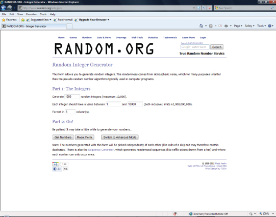
To avoid the paper cuts, you can assume that with the appropriate sampling frame, each student would coincide with a number (students 1 to 10,000). Another way to take a random sample would be to employ an electronic random number generator, like Random.org. Random.org uses true random number generation and is easy (and free) to use for most purposes. If you use the integer generator from Random.org to select a 10 percent (1000 people/units) sample from 10,000, what do you need to know? First, you need to plug in the total number of numbers you need (1000). Next, the program asks for the range of numbers needed. If the university has 10,000 students, the range would be 1 to 10,000. Figure 8.2 shows a screen shot of Random.org.

Figure 8.2. The Web site screen for Random.org.

Click on “Get Numbers,” and the screen will fill with 1000 integers all between the range of 1 to 10,000. Figure 8.3 shows the screen shot results for this specification. This is much simpler than drawing 10,000 names out of a hat.

Figure 8.3. The list of random numbers chosen from Random.org.

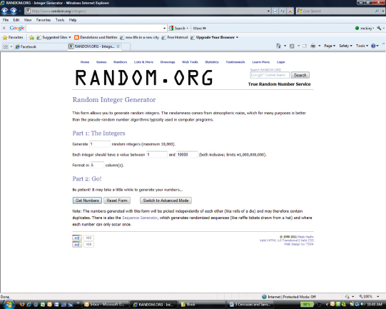
There is one problematic issue with a random integer generator, however. We change our example to select 50 numbers from a range of 1 to 100. Figure 8.4 shows this result.

Figure 8.4. Selection of a smaller sample using Random.org.

Do you notice anything about the distribution of numbers in Figure 8.4? It is likely that when choosing random numbers from a random number generator that integers will be repeated (like the numbers 6, 67, and 26 shown in Figure 8.4). That is problematic because you’ve set the parameters of the generator to match your needs. Since you will never know how many numbers will be repeated and if it will negatively impact your random selection, there is another way to use probability sampling that is helpful as populations increase.

Systematic Random Sampling

All probability samples use randomness as the basis for selecting observations. A systematic random sample does the same using a two-step process. Once you have a sampling frame—a list with all of the units in the population—the very first case/unit is selected randomly. Refer back to our example of taking a 10 percent sample of a 10,000-member university student body. Our sampling frame from the registrar’s office lists all currently enrolled students. Thinking that each name on the list corresponds to a number (from 1 to 10,000), we can use a random number generator like Random.org to select the first case. This is shown in Figure 8.5a. Using the integer generator (because we are selecting only one random number, there will be no problem with duplicate integers) to select one random number between 1 and 10,000, say we get the number 5398.

Figure 8.5a. Using Random.org to specify the first case of a sample.

Person 5398 on our list shown in Figure 8.5b becomes our random start. The second step in the process is to calculate a sampling fraction. A sampling fraction is calculated by taking the total number of the population and dividing it by the number of units/people needed for the sample: n.

Figure 8.5b. The first case in a systematic sample.

By dividing the total population (10,000) by our sample size (1000), we compute 10 as our sampling fraction. Since a random number (5398) has been generated for the starting number, each subsequent number is random. We begin by selecting person 5398 from the list for our sample and then take the sampling fraction to select every nth (or 10th) case until the end of the list is reached. Once 5398 is the selected person, 5408 is selected next, then persons 5418, 5428, 5438, and so on. Once we’ve hit person 10,000, we go back to the beginning of the list to select every 10th person until we get back to person 5398. (Since we started with number 5398, we have to make sure to systematically sample the cases “in front of” number 5398.)

Using SPSS to Obtain a Random Sample. 

Another way to obtain a random sample is to use the random selection process in SPSS. The procedure uses a process of nonreplacement so that the same case is not chosen twice. This means that once a case has been chosen, the remaining cases are selected from the group that remains (i.e., the number in the population minus the chosen case). Figure 8.6 shows the specification window.

Figure 8.6. The Selection window in SPSS that provides sampling.

Figure 8.7 shows the additional specification windows that appear once the SPSS user has requested “Select cases” from the “Data Analysis” window. As you can see in the example, we asked for “Exactly 50 cases” from the total number of cases in the population (1221).

Figure 8.7. The Random Sample menus in SPSS.

Telephone Polls (Random-Digit Dialing)

One of the ways social scientists conduct efficient probability samples is through the use of random-digit dialing. Most households have one telephone line given a unique 10-digit code (we called these telephone numbers). The 10-digit codes used as telephone numbers are more complex than just assigning households a unique identifier. The phone number is based in three parts: the area code, the exchange, and the four-digit random number. Together, these three parts create a number identifying roughly 96 percent of all American households. These numbers are also useful because both the area code and the exchange code are geographically based. Random-digit dialing allows scientists to program into software the area codes and exchanges that were needed to reach the appropriate sample populations for their research. For example, if we wanted to survey Seattle residents on their attitudes toward green energy initiatives, we could program the first three digits of the phone number to Seattle’s 206 area code. We could even program specific neighborhood exchanges to pinpoint areas even more precisely.

Using random-digit dialing gives researchers access to any household/number. Unlisted telephone numbers are equally likely to be dialed; therefore biases related to who has listed and unlisted numbers are eliminated. With the increasing use of cell phones, however, this process becomes more complicated. When researchers employ probability sampling, they have to make sure that every unit in the population has an equal chance of being chosen for the representative sample. In households that have multiple land lines and/or cell phones, the risk of duplicating people or households increases, impacting the representativeness of the sample.

Stratified Random Samples

As populations become larger and research questions more complex, probability sampling has evolved to take population characteristics into account. Stratified random sampling uses probability theory in a somewhat more complex way. The word strata means “layer.” You may think of stratification, or the rankings/layers of a society (e.g., richest to poorest, oldest to youngest, etc.). Depending on your research question, you may need to take this more complex approach. For example, if we are interested in how physics gets taught at the secondary level, we could do a probability sample of all secondary physics teachers in the United States. As we think about physics as a discipline, however, we might realize that it has an unbalanced gender ratio—men are more likely to teach physics than women. If we do a systematic random sample (or a simple random sample), we will have a representative sample of physics teachers. But what if our theory or previous research tells us that male physics teachers teach differently from female physics teachers? If physics teachers are 68 percent male and 32 percent female, we may not have enough variation between male and female to use sex as a variable. What if our random sample underestimates the percentage of female physics teachers? If sex is an integral variable to our research question, we need to make sure that we have enough variation between female and male to be able to use sex as a variable. Since significantly more physics teachers are male, we run the risk of getting more male respondents in our random sample and not enough female respondents.

Knowing that sex in an important piece of the research, we may want to employ a stratified random sample. A stratified random sample evaluates among the population the categories of a characteristic (stratum) that is important to the research. For our example, sex is a variable given two categories—female and male. In order to stratify by sex, we would need to know the proportion of the stratum in the population. Based on a report by the American Institute of Physics (White and Tesfaye 2010), we know that 68 percent of those teaching physics are male and 32 percent are female. When we use stratified random sampling, we sample with the same proportion of strata as the true value (parameter), eliminating statistical (random) error.

Rather than sampling the entire population, we would first create a sampling frame for each category of the variable for which we are stratifying. In our example, the variable for sex has two categories, so we would need two sampling frames—one for female physics teachers and one for male physics teachers. Once we have each group, we would randomly sample from each. Since each physics teacher has an equal probability of being chosen for the sample (because all are accounted for within the sampling frames), the sample is representative of physics teachers as a whole and can be generalized to the larger population of physics teachers. Stratifying a sample ensures that the sample is representative of the population as a whole while at the same time ensuring that the sample contains the appropriate variation for important variables.

Cluster Sampling

Cluster sampling is another two-step sampling process. What is unique about cluster sampling is that rather than beginning with individual units, we begin with aggregate units. By randomly selecting units, we can then survey the individual units within the randomly selected clusters and still have a random sample of individuals. Since each cluster has an equal chance of being chosen, by default, the individual units within the clusters also have an equal chance of being chosen, ensuring randomness.

For example, say that the United Methodist Church wanted to survey members on their attitudes toward politics. It is very difficult for the national denomination to maintain an accurate list of all United Methodists in the country, since people join congregations that are affiliated with the denomination, instead of signing up with the denomination. What the national denomination does have, however, is an up-to-date list of all of their church congregations. Using the sampling frame made up of all United Methodist churches in the country, researchers can randomly sample each church congregation. Once the churches have been randomly selected, it is easier to obtain the membership lists from each selected church, getting updated addresses for members and then sending each member a survey. Even though you are surveying people from the same congregation, as long as the congregation was chosen as a random cluster, the results of the survey will be representative of United Methodists as a whole—all members, via their congregation, have an equal chance of being selected. That is the key. There is an issue, however, of representativeness if your sample of churches includes several megachurches. Because megachurches have a disproportionate number of members (and they are not distributed randomly), the sample could be skewed. In order to correct for this, there is a sampling procedure that takes cluster size into account: probability proportional to size.

Probability Proportional to Size

When drawing from clusters, we cannot assume all clusters are the same size. This will impact the random sampling. Methodologists have taken this into account with probability proportional to size sampling. Probability proportional to size (PPS) sampling allows researchers to equalize clusters, making sure each cluster has approximately the same number of individual units, ensuring true random sampling. With PPS, a sampling fraction is calculated based on the size of the cluster relative to the size of the population. As with general cluster sampling, each cluster has the same probability of being included in the sample.

A good example of PPS sampling comes from the General Social Survey (GSS), which we have been using. Conducted by the National Opinion Research Center (NORC) in Chicago (see GSS 2010), the GSS is a semiannual survey that samples noninstitutionalized people living in the United States who are 18 years old and older. Based on U.S. Census data, PPS sampling draws from the full national population using probability statistics to obtain a sample of approximately 3000 people using geographic clusters (since it is nearly impossible to create a sampling frame of 308 million individual units). NORC uses a multistage PPS procedure as an advanced cluster sample (in effect, the United States is broken into geographic blocks that represent similar-size clusters). NORC divides the United States into primary sampling units (PSUs) based on counties. Each county has a total number of households, as determined by the most recent census. Counties with less than 2000 households are merged with adjacent counties to create similar-size PSUs. PSUs are randomly sampled, and then interviewers travel from the first dwelling unit in the block beginning at the northwest corner of the block and proceed in a specified direction until they have completed the block quota (canvassing the block finding the appropriate proportion of people, as designated by the census tract data). Therefore, a region, nation, and other very large areas can be broken into clusters with similar numbers of individuals so each cluster—and thus individual—has an equal probability to be chosen for the sample.

SAMPLING AND STATISTICS

Probability sampling not only allows us to collect representative data of populations, it also allows us to calculate how close we are to the actual (true) characteristics of the entire population. When we measure the “true” value of a variable within the population, we are measuring the parameter. The parameter is a “fixed” value, meaning that in the population there is one true value for that variable at that moment in time. Currently, the percentage of women to men in the United States is 51 percent to 49 percent, respectively. These percentages would be the true, or fixed value of women to men; they represent the parameters of the variable for gender. When taking a representative sample of the population, we are likely to slightly overestimate or underestimate the percentages of women and men (in other words, get a slightly higher or lower percentage of women and men than the parameter). We expect this since sampling deals with what we observe, or statistics.

Statistics are the observed values of a variable within a sample of the population. For example, the 2010 Census confirms that the consistent parameter (true value) of men and women in the United States is 49 and 51 percent, respectively. Looking at two probability samples of Americans gives us slightly different statistics—or observed values. The 2010 GSS sampled Americans finding 56.5 percent of their sample to be women and 43.5 percent men. The 2008–9 American National Election Study (ANES) counted 42.5 percent men and 57.5 percent women. Both surveys overestimate the percentage of women while underestimating the percentage of men in the population.

Again, getting statistics that slightly overestimate or underestimate the parameters of a variable is normal. When a sample includes a substantial proportion of the population, the statistic should be quite accurate: the larger the sample, the closer the statistic should be to the parameter. Sometimes we know the parameters, making it easy to compare to the statistics. Sometimes, however, we do not. For example, in national elections probability samples are taken regularly to determine the outcome of an election before the election happens. In the months leading up to a presidential campaign, a host of news agencies use random-digit dialing to collect data about voting preferences. Targeting approximately 1000 to 2500 adults over age 18, polls ask who you would vote for if the election were held that day.

Three organizations that polled Americans on their voting preferences on November 2, 2008, included Gallup, Diageo/Hotline Daily Tracker, and Reuters/C-SPAN/Zogby. These three organizations reported the statistics (observed values) of the percentage of the popular vote expected to go to McCain and Obama for November 2, 2008, and found in Figure 8.8.

Figure 8.8. 2008 preelection presidential poll statistics.

What’s nice about the observed values (statistics) listed in Figure 8.8 is that we will find out how accurate they are when the poll results (parameter) come in on that first Tuesday of November (designated as Election Day). Before that day, however, we can calculate how close the statistics are to the parameters—even though we do not know yet what the true value/parameter will be. The magic of mathematical probability theory allows us to calculate a confidence interval and a confidence level.

The confidence interval is an estimated range of values, based on the sample that should contain the actual population value a certain proportion of the time. A confidence level is the probability that the parameter (i.e., the “true” value) falls in that range (the confidence interval). For example, whenever political pollsters report their results, they give a range of percentage points (e.g., “plus or minus 2 percentage points”). The 2008 preelection results given in Figure 8.8 were reported with various margins of error. The percentage points given help us to create the range (confidence interval) for which we expect the parameter to fall. We take the statistic and we add the margin of error points to the statistic (e.g., “plus 2 percentage points”) and subtract the margin of error points (e.g., “minus 2 percentage points”) to create the range within which we expect the parameter to fall. Figure 8.9 calculates the confidence intervals for each of the three organizational polls.

Figure 8.9. 2008 preelection presidential poll statistics with confidence intervals.

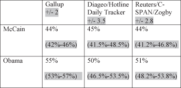
Thus, according to the example in Figure 8.9, a “95 percent confidence interval” would indicate which two percentage values that would contain the actual population opinion value 95 times out of 100. If the poll predicted McCain getting 44 percent of the popular vote, we would be 95 percent confident that the actual popular vote would fall between 42 percent and 46 percent. These values are shown in Figure 8.9 by the ±2 indicated as the margin of error in the Gallup Poll.

After Election Day we can evaluate how close the statistics (observed values) come to the parameter (the actual percentage of those who voted for McCain or Obama). Figure 8.10 reports the confidence intervals, as well as the actual percentage of the popular vote each candidate received.

Figure 8.10. 2008 preelection presidential poll statistics with confidence intervals and parameter.

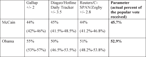
Clearly the parameter (true value) of the percentage of the popular vote for McCain and Obama fall within each of the three confidence intervals calculated on the preelection poll statistics.

POTENTIAL BIASES IN PROBABILITY SAMPLES

We have tried to make clear that for scientific research to be done on large populations (small ones too), representative data are useful. The only way to obtain representative data is to use random sampling techniques—probability sampling; otherwise, regardless of how well a survey is written, the data obtained cannot be generalized to the population. Once a probability sample has been diligently selected, there are a few things that can impact the representativeness, and thus the generalizability, of the sample. These issues include nonresponse, selective availability, and areal bias.

Nonresponse

We’ve outlined the steps needed to select a representative sample of a population. Even the most diligent researchers, however, must monitor the amount of nonresponse—people who do not respond—within the sample. In any data collection there will be people who refuse to participate, people who are unavailable to participate, and/or people who are too ill to participate. These people are the “nonresponders.” Researchers expect some people selected by probability sampling to simply not answer their phones, not return a survey, and so on. Unfortunately, if there is significant nonresponse, we cannot generalize the results of the data collection to the population because people who do not respond are not distributed randomly. Thus a high rate of nonresponse results in a sample bias. There are actually patterns or groups who are less likely to respond—younger people, males, residents of cities, conservatives, the very poor, and/or the very wealthy.

Selective Availability

Somewhat akin to nonresponse is the problem of selective availability. Although they may be willing to respond to a survey, some people are just difficult to find, including those who are institutionalized and those who are simply less available, resulting in selective availability. Institutionalized populations—people in the military, people who are incarcerated, and people who are in college—are less available and therefore less likely to participate, which again, can negatively impact our ability to generalize findings to a whole population.

Areal Bias

Another type of bias that can hurt the generalizability of a probability sample is areal bias, a geographic bias that occurs because sampling is based on geographic units. Stark and Roberts (2002) outline some of the issues regarding areal bias in the GSS’s primary sampling units (PSUs) from the 1990s. In selecting random units, none of them happened to fall in two regions: the western region or the Miami region. This means that the results of the GSS can be generalized to residents in America but cannot be used to generalize about certain subgroups including Mormons, cattle ranchers, and Cuban Americans. These specific groups are underrepresented in the data.

NONPROBABILITY “SAMPLES”

The previous examples of probability sampling are the only sampling techniques that allow researchers to generalize to a population. Unfortunately, we sometimes run into data that are collected using nonprobability “samples” to generalize to some population (often by well-meaning but ill-informed people). If random sampling—or probability sampling—is not used, then the data taken cannot be generalized to any population because the sample is not representative of any population. Just because we have data gathered from people within the population does not mean it is representative, and thus generalizable, to that population.

What if we are interested in how students think about the alcohol policy at our university? We develop a survey about the alcohol policy and then ask the students in our classrooms to complete it. We then take the data, analyze it, and report to our colleagues that our university’s students believe that the alcohol policy is a good policy. What is the problem with doing this? Do the students in our classrooms represent all the university’s students? They are students at our university. Do not they represent our students? The question to ask is “Did every student at our university have an equal opportunity to be chosen to take our survey?” If we only took our own students (even if we asked our faculty friends to give the survey to their students, too), then they are not representative of the university’s students as a whole, and any data we get from them cannot be considered representative. The data may tell us something about the students who responded to the survey but does not represent the students at the university and therefore cannot be generalized to the university student population. In such cases, the findings of our research could only be generalized to the set of students who took the survey. Data that cannot be generalized to the target population are less meaningful than representative data because we do not know who is represented by the results of the data.

A classic example of this problem lies in the popular prediction of a winner for the 1936 presidential election between Alf Landon and Franklin Delano Roosevelt (FDR). In several earlier elections, the largest periodical of the day, Literary Digest, had accurately predicted the winners of presidential elections. Literary Digest created an ambitious method to determine the presidential election outcome. Sending 10 million ballots to Americans, the periodical received 2 million responses—a fair response rate. The results of the poll showed Alf Landon with 57 percent of the popular vote and FDR with 43 percent of the popular vote. It looked as if Landon would win in a landslide over FDR. When Election Day rolled around, however, Landon carried only two states and FDR won 61 percent of the popular vote. How could Literary Digest’s statistics have been so far off the parameters?

The first question to ask is how did Literary Digest get a list of addresses for 10 million Americans? What was their sampling frame? Literary Digest got lists of all automobile owners and all telephone subscribers in order to send out their ballots. Are these two groups representative of all Americans? Think about what you know about the country in 1936. The United States was in the midst of the Great Depression. Did most Americans have their own cars and/or telephones? In the midst of the Depression in the United States, only those considerably more wealthy than average received ballots. There is a correlation between wealth and voting Republican, which may explain the inflated statistics favoring Alf Landon. Obviously these groups were not representative of the population as a whole; thus the results of the survey were meaningless.

In their defense, Literary Digest did not use probability sampling. They were using some of the most up-to-date techniques of taking data, but probability sampling was not in common use at the time. What we know now is that even with a much smaller sample (for example, national election polls draw on just 1000 people from a population well over 300 million), as long as each unit in the population has an equal chance of being selected for the sample, a probability sample can accurately predict/describe the entire population.

Convenience Samples

As we’ve noted previously, social researchers use words very precisely. When discussing samples, there is an expectation that a sample is equal to a representative group of units from some larger population. In popular usage, however—sometimes creeping into the vocabulary of the sciences—the word sample is often used to refer simply to a group of units (most often a group of people who may or may not be members of the population of interest, but who are not necessarily representative of that population). Technically, groups of units or people from the population who have not been randomly selected are not a sample; they are just a group of people. Data taken from this type of group are generally not useful because the results of the data cannot be generalized to any population—even the one to which they may belong.

The most egregious type of a nonsample “sample” is the convenience sample. Just as the name implies, units are selected conveniently, drawing on those that are most available. Even when some of the units are found within a common population, if they are not chosen randomly, the units are not representative of the population (or what we call a relevant population). Because the units are not representative of a relevant population, the data taken from them is not generalizable to any relevant population.

A great example of this would be the late-night talk show host who walks outside of his studio to ask people questions. A couple of years ago one of these hosts asked for graduates in his audience to answer the question, “How many planets are there?” In the seven or eight clips that were shown on television, none of the graduates could accurately identify the number of planets (this example predates Pluto’s demotion from a planet). The graduates’ answers caused great hilarity for the audience. When the host came back into the studio, his response (and that of the audience) highlights the problem with a convenience sample. The late-night host noted, “Look at the state of American education!” The audience clapped raucously in agreement with him that graduates from American schools—including high school, college, and one graduate student—could not identify something simple like the number of planets in our solar system. The host was generalizing to all people with educations from American institutions. Did the people he interviewed on camera represent all people with an American education? No, but both he and the audience (without too much thought) generalized his findings to the whole population of everyone who has an American education. We do not expect professional comedians and television hosts to know or use probability sampling. We must also recognize that journalists and even some scientists not trained in taking reliable sampling data from people may not understand the principles behind probability sampling and generalizing from a group of people/units to any larger relevant population.

Quota Sampling

Another type of a so-called sample that has a veneer of scientific accuracy is quota sampling. Quota sampling is based on a matrix that describes certain characteristics of a target population. The key to quota sampling is to find a current and accurate accounting of these characteristics. Like stratified random sampling, quota matrices rely on up-to-date information regarding the proportion of demographic characteristics in a target population. For example, several malls have video stations where you may be asked to participate in a study showing movie trailers to get your reaction to the films. These stations are usually staffed by people with a clipboard or electronic tablet and a quota matrix. The matrix will have a breakdown of the characteristics that are important to the organization collecting data. For films, perhaps market researchers want to find out how a general population responds, so a matrix will target perhaps 100 people, broken into several categories. If 51 percent of a population is female, the data collection will ask for 51 females to view the film trailers (and then 49 males). Each sex category may also be further broken down into age groups. So of the 51 women who are supposed to view the film trailers, perhaps 20 percent should be under 18, 30 percent between 18 and 25, 40 percent between 26 and 45, and 20 percent over 45, each percentage representing the proportion of those age groups who attend movies. So the person stationed at the video booth would need to have 10.2 women who were under 18, 15.3 women who were 18 to 25 years old, 20.4 women 26 to 45 years old, and 10.2 percent of women who are over 45 years old. Of course getting those extra “point 2s” may be tricky.

From gender and age, the matrix could be further broken down into more categories, for example race. Once each category has been filled, the data are collated and taken back to their respective organizations, where decisions are made based on the results (which are not random, even though the data are from people who represent each category). Although quota sampling resembles probability sampling, it still is not a scientific substitute for probability sampling. It is difficult to find accurate and current information on the population proportions of characteristics, and again, not everyone in those categories has an equal chance of being selected, so they cannot represent any type of relevant population, and thus the findings cannot be generalized to any relevant population.

Snowball Sampling

The remaining type of nonprobability “sample” can be helpful when doing exploratory research—when you do not know enough about a population to undertake a full-scale data collection using a probability sample. Snowball sampling is also useful for learning from special populations that may be difficult to locate (e.g., drug users, illegal aliens, sex workers, etc.). Like the “snowball effect,” snowball sampling occurs when researchers begin with one person of interest and ask that person to refer others from the population or who share the characteristics to be studied to the researcher. Although this type of group can give valuable insights, the data collected cannot be generalized to others—even those who share the same characteristics being studied.

For example, how do people decide to place their loved ones in a nursing home? Having no type of sampling frame that would identify people facing the decision to place loved ones in a nursing care facility, snowball sampling would be a good way to begin to collect data on this special population. Identifying support groups through hospitals or nursing care facilities may be a good way to begin to find people willing to be interviewed about making this decision. Once interviewed, those in the process of placing a loved one in nursing care mayknow of others experiencing a similar situation and choose to refer them to the researcher. Snowball sampling can be quite helpful in this type of research context.

Note

¹ The U.S. 2010 Census form is reproduced here by permission.