
DATA MANAGEMENT UNIT A: USE AND FUNCTIONS OF SPSS1
MANAGEMENT FUNCTIONS
In this section, we cover the essential functions that will allow you to get started right away with your analyses. Before a research procedure is created, it is important to understand how to manage the data file.
Reading and Importing Data
Data can be entered directly into the spreadsheet or it can be read by the SPSS program from different file formats. The most common format for data to be imported to SPSS is through such data programs as Microsoft Excel or simply an ASCII file where data are entered and separated by tabs. Some large data files, like General Social Survey (GSS), have already been converted into SPSS file format and are available simply by downloading the data from the Web site.
Using the drop-down menu command “File-Open-Data” (initiated in the upper left of the main menu ribbon in either Data View or Variable View) creates a screen that enables the user to specify the type of data to be imported (e.g., Excel, Text, etc.). The user is then guided through an import wizard that will translate the data to the SPSS spreadsheet format.
Figure DMUA.1 shows the screens that allow you to select among a number of “Files of Type” when you want to import data to SPSS. These menus resulted from choosing “File” in the main menu and then “Open Data.” The small drop-down menu allows you to choose a number of different file types to import data. As you can see in Figure DMUA.1, there are many common types including SPSS files, Excel files, and a number of others including text files (that you can see if you use the navigation bar within the small Files of Type menu).
Figure DMUA.1. The SPSS screens showing import data choices.

Sort
It is often quite important to view a variable organized by size or other consideration. You can run a statistical procedure, but it is a good idea to check the position of the data in the database to make sure the data are treated as you would expect. In order to create this organization, you can “sort” the data entries of a variable in SPSS.
Figure DMUA.2 shows part of the 2010 GSS database—a sample (N = 10) of cases and two variables: health of respondent (“health”) and sex of respondent (“sex”). As you can see, these two variables consist of a series of numbers that represents the coding of the data. For sex, the codes are Male = 1 and Female =2.
Figure DMUA.2. The SPSS screen showing the unsorted “Sort-example” data.
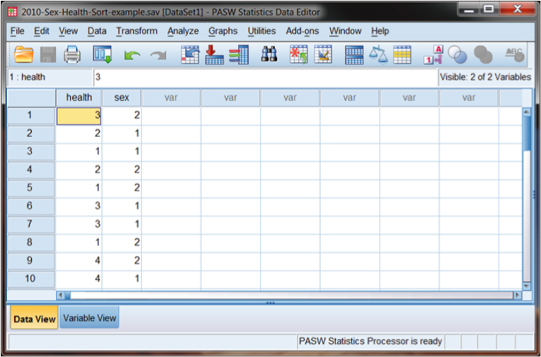
Figure DMUA.3 shows the Variable View of the spreadsheet that allows you to examine the codes for health. If you click on the cell for “health” under its Values column, you will see a separate menu box that lists the values of each of the numbers in the database. This box shows that 1 = Excellent, 2 = Good, and so forth.
Figure DMUA.3. The SPSS screen showing the Value Labels for the health variable.

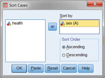
Sorting the data in SPSS is straightforward. The user can simply select “Data” from the main menu bar, and then “Sort.” This results in the screens shown in Figures DMUA.4a and DMUA.4b in which we have selected sex as the sorting variable. When you select “Data–Sort Cases” as shown in Figure DMUA.4a, you will then be shown the separate menu box shown in Figure DMUA.4b in which you can select “sex” by simply highlighting it and moving it to the Sort by: window using the arrow key.
Figure DMUA.4a. SPSS data screen showing the “Sort Cases” function.

Figure DMUA.4b. SPSS data screen showing “Sort Cases” specifying sex as the sorting variable.
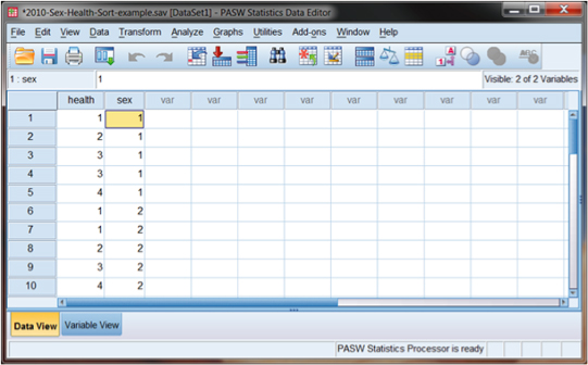
If we choose sex, as shown in Figure DMUA.4b, we can specify a sort that is either “Ascending” (alphabetical order beginning with “A” if the variable is a string variable or starting with the lowest value if it is a numerical value) or “Descending.” Selecting “sex–Ascending” results in the screen shown in Figure DMUA.5. There are many reasons to perform a sort, among which is that you can inspect the values of a related study variable on values of the sorted variable. Thus, for example, you can see in Figure DMUA.5 that among this example set of cases, males’ (sex = 1) health is generally a bit poorer than females (sex = 2). The data show that the males’ health values appear to be a bit higher (and therefore poorer) than those of the females.
Figure DMUA.5. The SPSS screen showing variables sorted by sex.

SPSS allows multiple sorts. Figure DMUA.6 shows the specification window for a multiple sort first by sex and then by health. Users can generate this result simply by listing multiple variables in the “Sort Cases–Sort by” window. Note that the each of the variables can independently be sorted in ascending fashion (signified by an “A” next to the variable name) or descending (signified by a “D”). Figure DMUA.6 also indicates the nature of the variable (string or numeric) by the small symbols next to each variable. Sorting (in either ascending or descending order) will therefore appropriately arrange the variables according to their type.
Figure DMUA.6. The SPSS Sort Cases window showing a sort by multiple variables.
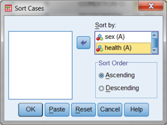
Figure DMUA.7 shows the result of this multiple sort. As you can see, the health values are nested within each category of sex. This makes visual inspection of the data somewhat easier. Compare this screen with the one shown in Figure DMUA.5. Sorting by multiple variables allows you to see the patterns a bit more clearly.
Figure DMUA.7. The SPSS screen showing the database results of sorting by multiple variables.
ADDITIONAL MANAGEMENT FUNCTIONS
SPSS is very versatile with handling large data sets. There are several useful functions that perform specific operations to make the analyses and subsequent interpretation of data easier. We do not cover all of these, but the following sections highlight some important operations.
Split File
A useful command for students and researchers is “Split File,” which allows the user to arrange output specifically for the different values of a variable. Using our sort example from Figure DMUA.5, we could use the “Split File” command to create two separate files according to the sex variable and then call for separate statistical analyses on each of the related sets of cases of the other study variable (in this case, health).
By choosing the “Data” dropdown menu, we can select “Split File” from a range of choices that enable us to perform operations on our existing data. Figure DMUA.8 shows the submenu for “Data” with “Split File” near the bottom.
Figure DMUA.8. The “Split File” option in SPSS.

When we choose “Split File,” we can then select which variable to use to create the separate data files. This is the Organize output by groups button shown in Figure DMUA.9. As you can see, if you choose this button, you can specify “sex” by clicking on it in the left column and moving it to the “Groups Based on:” box by clicking the arrow button.
Figure DMUA.9. Steps for creating separate output using “Split File.”

As Figure DMUA.9 shows, we selected the option “Organize output by groups” and then clicked on the variable “sex” in the database. By these choices, we are issuing the command to create two separate analyses for whatever statistical procedure we call for next, since there are two values for the sex variable (“1” and “2”). When we perform a split file procedure in SPSS, it does not change the database; rather, it simply creates separate output according to whatever statistical procedure you want to examine. We discuss many such statistical procedures in other sections. For now, it is important to understand that SPSS has this useful function.
As an example, the researcher might be interested in whether the health ratings differ by sex. We inspected the data in this way by looking at the screen in Figure DMUA.7. However, researchers cannot trust their eyes when it comes to analyzing and finding patterns in data. We can use some of the SPSS analysis functions to help provide a more objective way of examining the health differences by sex category.
With the file split by sex, you can call for SPSS to create separate frequency tables of health ratings. Figure DMUA.10 shows the menu screen that you can create to provide these tables. You obtain the Frequencies menu through the command ribbon in the original spreadsheet window.
Figure DMUA.10. The SPSS Frequencies menu.

As you can see in Figure DMUA.10, we have specified frequencies for the health variable. Recall that SPSS has already split the file, even though this is not indicated on the menu. With the Frequencies window, you can choose which analyses you would like to see by selecting from a list under the Statistics button in the upper-right corner of the Frequencies menu. Since the health rankings are technically ordinal rankings, we will simply use the default analysis which is a frequency table (note the checked box, “Display frequency tables,” in the lower left of the box.
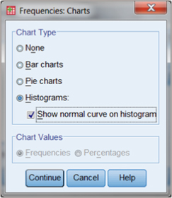
If you want a graphic display as well as a table of percentages, we can select the Charts button just below the Statistics button. Figure DMUA.11 shows the menu that appears when you choose the Charts button. Note that we have called for a histogram that includes a superimposed normal curve line.
Figure DMUA.11. The SPSS Frequencies: Charts menu.
When we make these selections, SPSS returns separate frequency analyses for males and females, since we have split the file by sex. As you can see in Figure DMUA.12a (the first part of the output, for Male respondents), most (three of five) of the cases show Fair or Poor health ratings. The frequency table (first panel of Figure DMUA.12a) is the numerical equivalent of the histogram. As you can see, two of the respondents indicated “Fair” health.
Figure DMUA.12a. The SPSS split file results for health ratings (Male).
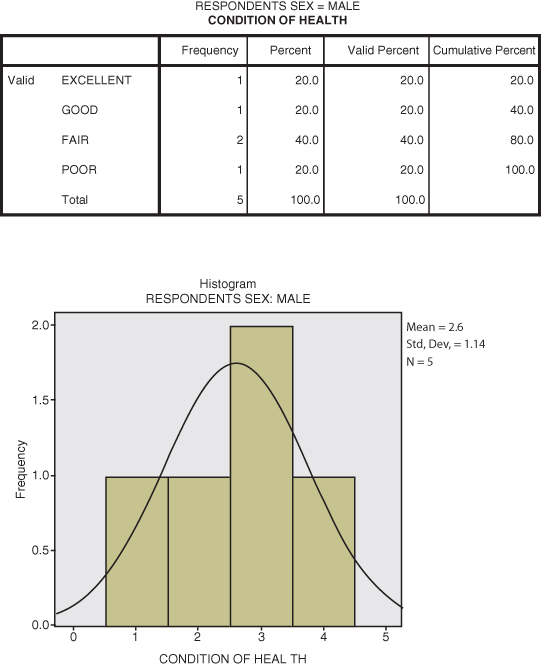
Figure DMUA.12b shows the second part of the split file frequency results. As you can see from the histogram, the cases tend to indicate better health ratings than the male findings. Both histogram and frequency table show more cases among the lower (i.e., better) health ratings. Two of the cases reported excellent health.
Figure DMUA.12b. The SPSS split file results for health ratings (Female).

Please note that when you use this procedure, it is necessary to “reverse” the Split File steps you used after you have created the desired output. Otherwise, you will continue to get “split results” with every subsequent statistical analysis you specify. SPSS will continue to provide split file analyses until you “turn it off” by selecting the first option, “Analyze all cases, do not create groups” at the top of the option list in the Split File submenu. You can see this option near the top of the submenu in Figure DMUA.9.
Compute (Creating Indices)
One of the more useful SPSS management operations is the Compute function, which allows the user to create new variables from existing variables. For this example, we use two variables from the 2010 GSS database that measure socioeconomic status (ses) to compute a new variable.
Socioeconomic status (ses) is a central concept in social science. It is a broad measure of one’s social standing in that it measures education, income, and occupational prestige. Researchers have devised a way to combine these measures to yield one index that serves as a general indicator of social standing.
The GSS, as we noted earlier, provides a ses measure for all respondents. The sei variable is an index measure of the respondent’s ses, and pasei is the respondent’s father’s ses rating. By using SPSS to divide the respondent’s ses index by the father’s ses index, we can create a new variable (generational ses mobility or “gensei”) that indicates the extent of social mobility that has occurred from father to respondent. If the resulting number is greater than 1.0, then the respondent has eclipsed the ses of the father.2
We can compute gensei using the main menus in SPSS. At the main menu, select the “Transform” and then “Compute Variable” option. This will result in a dialogue box like the one shown in Figure DMUA.13. In this example, we can create a new variable (“gensei”) by dividing the current “sei” variable by the “pasei” variable. The first step is to name the new variable by entering it into the “Target Variable:” the window at the upper left of the screen. Then, you can create a formula in the “Numeric Expression:” window. As Figure DMUA.13 shows, we clicked on “sei” from the list of variables and placed it in the window by clicking on the arrow button. Then, we entered a “/” mark using the keypad below the window. Last, we placed “pasei” in the window to complete the formula: sei/pasei.
Figure DMUA.13. SPSS screen showing the “Compute” function.
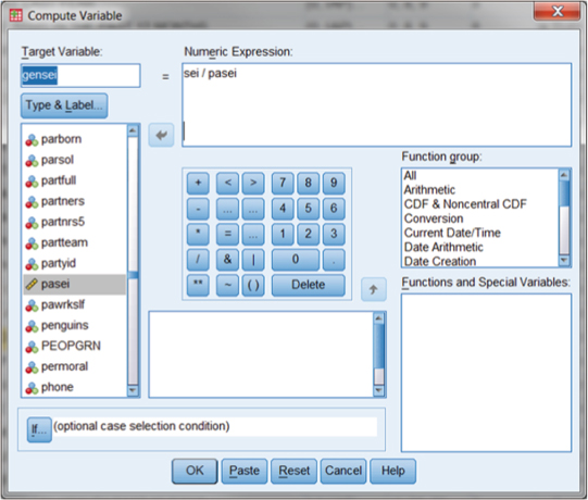
As you can see from the screen in Figure DMUA.13, you can use the keypad in the center of the dialogue box for entering arithmetic operators, or you can simply type in the information in the “Numeric Expression:” window at the top. You will also note that there are several “Function group:” options at the right in a separate window. These are operations grouped according to type. Scrolling to the bottom allows the user to specify “statistical functions” like means, standard deviations, and so on. You can select whichever operation you need and enter it into the Numeric Expression window by clicking on the up arrow next to the Function Group window.
ANALYSIS FUNCTIONS
Over the course of our study in this book, we will have practice at conducting statistical procedures with SPSS. All of these are accessible through the opening “Analyze” drop-down menu as shown in Figure DMUA.14. The screen in Figure DMUA.14 shows the contents of the Analyze menu. We will not be able to cover all of these in this book, but you will have the opportunity to explore several of the submenu choices.
Figure DMUA.14. The SPSS Analyze menu options.

DATA MANAGEMENT UNIT A: USES AND FUNCTIONS
| Use and Function | SPSS Menus |
| Read and Import data | File–Open Data |
| Sort the database according to a variable | Data–Sort Cases |
| Arrange output according to different categories of a variable | Data–Split File–Organize output by Groups |
| Compute a new variable or index | Transform–Compute Variable |
Notes
1 Some of the material in this section is adapted from Abbott (2011) with permission of the publisher.
2 In this example, we are not considering the age, gender, or sex difference of respondent vis-à-vis the respondent’s father. The example illustrates only the process of computing a new index from existing variables.