Key 3
Discover where and when to buy
The previous key showed you how to read any housing market and predict the likely direction of price and rent changes in any suburb or town. This key shows you:
 the different types of housing markets and how they work
- when they are likely to provide the best returns.
We look at owner-occupier-dominant and renter-dominant markets and show you how to find markets that are forecast to perform well and avoid those where price falls are likely.
The three dynamics of the housing market — people, purchasing power and properties — work together to cause price and rent changes and we can group households together by the way these factors combine. For example, first-home buyers are heavily reliant on the cost and availability of housing finance, while potential retirees have no need for finance at all and usually downgrade when they buy their final home. There are also times when high overseas immigration leads to a rise in rental demand in some locations, or when opportunity seekers move to a mining town or tourist resort and boost rental demand.
Understand different market dynamics
By understanding the dynamics of each of the different types of households, you will know when to invest in certain suburbs and when not to.
First-home buyer markets
The high cost of buying a home in Australia means that virtually every first-home buyer engages in a reluctant trade-off between that ideal home in a location they desire and the less satisfactory home in a location they can afford. Not only does this restrict first-home buyers to lower-priced houses in the outer suburbs and units along the major transport corridors of our cities, it also means that they will move to a better home in a more desirable location as soon as their circumstances permit.
Since 1991, first-home buyers have only made up about 15 per cent of property purchases annually, and they entered into just one-fifth of total housing finance commitments. Yet history shows that whenever their numbers rise significantly above those proportions, first-home buyers have acted as a growth catalyst, initiating price rises at the low end of the market that create equity for previous first-home buyers and precipitate movement upward all the way through the housing market.
Many new households will rent for years before they feel the need or are able to buy their first home, so their demand for housing flows largely into investment properties. The crucial demand dynamic in first-home buyer markets is the number of new or renting households that aspire to become homeowners. Our population growth from births has been slowly rising for many years, creating a steady increase in potential first-home buyers, but the rate of overseas migration has varied considerably. Many migrants arrive here in ready-made households and it takes them a few years to get settled to the point where they can successfully apply for a home loan. This means there is a time lag of three to four years before most overseas arrival households can hope to become first-home buyers.
Figure 3.1 shows the dramatic increase in the number of prospective first-home buyers that occurred in 2012 and 2013. This was mostly due to a rise in the number of overseas arrivals three to four years before.

Figure 3.1: prospective first-home buyers' origins
Source: Australian Bureau of Statistics.
Even though our population growth rate has now slowed to its long-term average of about 1.6 per cent per annum, when increases in overseas migration occur, they often lead to housing booms a few years later.
Although homeownership is an integral part of the great Australian dream it often seems to be out of the reach of first-time buyers. Lower-priced housing markets can experience little to no growth for years on end, and even occasionally suffer considerable price drops if buyers fall away. Whenever this happens, fingers are pointed at possible culprits such as:
- housing unaffordability
- high deposit requirements
- interest rates
- lack of government incentives
- economic slowdowns.
Although the cost of their first home must seem incredibly high for aspirational owners, they are not being asked to pay for it in cash. It is not the price of the property that deters them from purchase, but two components of the price:
- the monthly payment, which is related to the amount of finance that the lender is prepared to provide
- the deposit, which is the unfinanced portion of the purchase price.
Loan repayments are linked to the borrower's income, current interest rates, the period of the loan and the amount financed, but housing deposits are an artificial construct used by lenders to minimise risk and maximise return. They do this by setting the percentage of the property's value for which they are prepared to provide finance. When money is tight or lenders are nervous, they restrict finance by increasing the percentage of the price that borrowers have to find themselves. The effect of this tactic is shown in Figure 3.2, where high deposit requirements in some years have acted like a barrier, putting many budding first-time buyers out of the race.

Figure 3.2: the first-home buyer deposit barrier
Source: Australian Bureau of Statistics; housing data provided by Australian Property Monitors.
Although the Reserve Bank might cut interest rates to historical lows, it requires more than the cost of finance to enable aspiring first-home buyers to enter the market; they must also be able to raise the deposit. Figure 3.2 shows why first-home buyers did not participate in the Sydney housing boom in 2014: the deposits required by lenders were such a disincentive. If the required deposit is more than 80 per cent of a household's annual income it becomes too difficult. The figure also shows that in 2001 and 2008 the amount of household income required as a deposit fell to 30 per cent or less and led to first home buyer booms in those years.
When finance is easy and lenders are full of confidence about the housing market, they will finance about 90 per cent of the purchase price, even for a first-home buyer. This was the catalyst for the booms in first-home buyer markets in 2001 and 2008, although there were other factors that contributed to those booms, such as low interest rates and increases to the First Home Owner Grant.
How does an increase in a group of homebuyers normally comprising just 15 per cent of housing purchases precipitate a boom in the housing market? It's because the rules change. Low interest rates, increased home buyer grants and relaxed minimum deposit requirements, when they occur, apply to all prospective first-home owners, and if it's easier for one, it's easier for all. In addition, people with similar demographics tend to act together — when some lead, the rest will follow.
This is called the cohort effect, and it has a dramatic impact on first-home buyer markets when it occurs. The influx of buyers at the low end of the market enables existing owners to take advantage of the increased prices and upgrade to a bigger home or a better location. The owners of the homes they in turn purchase also then upgrade, and because each successive wave of upgraders has access to larger amounts of equity, prices escalate upwards along with values. By the time this wave of price-growth has made its way to the top echelons of the housing market, it will have already deserted the first-home buyer suburbs where it all started, which means that timing is everything.
Figure 3.3 shows how the growth in numbers of first-home buyers in 2000 to 2002 and 2008 to 2009 was accompanied by rising median house prices generally. These increases were across the board, working their way upwards through the housing markets from lower median-valued localities to higher-priced ones.
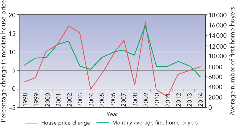
Figure 3.3: first-home buyer–led housing booms
Source: Australian Bureau of Statistics; housing data provided by Australian Property Monitors.
If prospective first-home buyers' desire for ownership is matched with increased government incentives, a period of low or reduced interest rates and lower deposit requirements, then the number of first-time homeowners swells dramatically. The good news for investors is that the longer such a mix of buyer incentives is delayed, the greater the pent-up demand for first-home purchases and the bigger the housing market boom that follows.
Upgrader markets
First-home buyers are constrained by the cost and availability of finance, so their first home may not be their preferred type of dwelling, or in an ideal location. This means that, usually after an average of four years has passed, they tend to move to accommodate a growing family's space and schooling needs, or to be closer to work, or family and friends. They may make several moves as their housing needs change and their ‘perfect location’ changes with their lifestyle and aspirations. We call these homeowners movers and improvers or upgraders. They comprise all those households that have made the transition to their second or third home, but are still paying off their mortgage. They represent about four million households, which is well over one-third of all households in Australia. As time passes they become progressively more financially secure and less at the mercy of interest rates.
Both their repayments and the passive growth in the housing market increase the equity they have in their home. Instead of needing a deposit to buy another home, they use this equity in the home they sell as a deposit. In addition they have acquired a proven repayment record and their loan repayments are gradually reducing as a percentage of household income. For this group of homeowners, affordability now becomes a measure of the equity in their home compared with the price of a new home and their ability to meet the new loan repayments. It means that each move is usually upward to a more desirable home or a more sought-after location.
This continual turnover of properties presents excellent opportunities for investors, because owner-occupiers buy and sell properties for personal reasons. It may be a buyer's market rather than a good time to sell, but many homeowners would not be aware of this. The area they move to may be a seller's market, and, again, they may be unaware. This is why investors who research these facts will always achieve more than the long-term growth rate in any area, because they are buying and selling at the right time to make the maximum gain.
One of the main causes of the Sydney housing boom in 2013–14 was established owner-occupiers who took advantage of lower interest rates and their improved financial conditions to upgrade to a bigger house in a better location, with the bank lenders willing to provide finance to established homeowners.
We can predict when and where such upgrader-led booms will occur. The best time to buy in upgrader markets is when:
- There has been an extended period of little to no growth in the market.
- Economic conditions are stable and unemployment levels are low.
- Housing finance is freely available to existing homeowners.
The issue is that you don't buy an entire city; you buy a property in one suburb. If this information is to be of value you need to know which suburbs are likely to rise in price, when this is likely to occur and how long it is likely to last. Although the median price-growth in the Sydney market was about 17 per cent in 2013 and 11 per cent in 2014, these modest numbers disguised some huge variations in house prices, such as those shown in Table 3.1.
Table 3.1: Sydney's best and worst performers 2012 to 2014
| Year | Best performer | Price rise in year | Worst performer | Price fall in year | Difference in performance |
| 2012 | Cabarita | 30% | Edgecliff | −27% | 57% |
| 2013 | Rhodes | 40% | Abbotsford | −10% | 50% |
| 2014 | Edgecliff | 45% | Tamarama | −7% | 52% |
Source: Housing data provided by Australian Property Monitors and Property Power Database, Property Power Partners.
The difference between the best and worst performing suburb in each year was quite staggering — it was 50 per cent or more! While some suburbs started rising in price during 2012, most were still falling in value; but even during 2014, when most suburbs were rising in price, some were falling. Most suburbs only rose in price in one or two of the three years, and many only went up in one year, to fall in value the next. There were some suburbs where house prices rose in every year from 2012 to 2014, but not very many, and some suburbs hardly went up in price at all.
If you jumped into the Sydney market in 2013 you may have done very well, or you may have achieved very little overall growth. How would you have any idea of which suburbs were most likely to rise in price and which to avoid?
Key 2 shows how to read the house or unit market in any suburb by the relationship of listings to sales. There are five types of markets: stressed and buyer markets have a surplus of properties for sale, neutral markets are in balance, and seller and boom markets have a shortage of properties for sale. Table 3.2 shows how to read suburb house or unit markets quite quickly by seeing whether there is a surplus or shortage of stock, and whether prices are likely to be rising or falling as a result.
Table 3.2: how to read housing markets
| More current listings than annual sales | About the same | More annual sales than current listings |
| Stock surplus prices falling | Balanced stock no change to prices | Stock shortage prices rising |
Source: Property Power Database, Property Power Partners.
Had you done this exercise in 2012, it would have helped to identify those Sydney upgrader suburbs that were about to boom and which ones to leave alone, as Table 3.3 indicates.
Table 3.3: reading the Sydney upgrader housing market 2012 to 2014
| Year | Best performer | Market reading | Worst performer | Market reading |
| 2012 | Cabarita | Stock shortage | Edgecliff | Stock surplus |
| 2013 | Rhodes | Stock shortage | Abbotsford | Stock surplus |
| 2014 | Edgecliff | Stock shortage | Tamarama | Stock surplus |
Source: Property Power Database, Property Power Partners.
House prices in Cabarita rose by over 30 per cent in 2012 because there was a huge stock shortage, while they fell by nearly the same amount in Edgecliff, where there was a high surplus of stock. By 2014 the situation had reversed itself, and Edgecliff now had an acute stock shortage that caused prices to rise by 45 per cent in one year. Such high price-growth is sweet but it doesn't last long, once again demonstrating the importance of timing the market.
You now have some simple, logical techniques to use when it appears that upgraders may be on the move and prices may change as a result.
Retiree markets
Some housing markets have provided excellent returns when growth was hard to find elsewhere. Seaside resorts such as Byron Bay, Coffs Harbour, the Gold Coast and Sunshine Coast enjoyed spectacular periods of growth in the recent past, but the data also tells us that growth in these markets inexplicably stopped even though the rest of the market was booming. The reason for their growth was their popularity as retirement destinations and the cause of their decline was when they stopped being attractive to retirees. Potential retirees make up one-fifth of the housing market; their houses are mostly owned without debt, they are located in many of the higher priced localities of our major cities, and the number of people approaching retirement age as a proportion of our population is actually increasing.
Australians have always looked to retirement with hopes for security, health, independence and sufficient fitness and finances to enjoy their extra free time. The prospect of selling the family home with its comforts and memories is another matter, often dreaded and put off as long as possible. Eventually, a number of factors can force their hand:
- health and money issues
- maintenance of a larger-than-necessary home
- the changing nature of the local area.
When they decide to seek a new location they'll search out areas that offer:
- better lifestyle
- appropriate health, recreation and entertainment facilities
- demographically similar neighbours.
This last factor is the most important, and explains the extremely high growth in retiree housing markets that have occurred in the past — retirees tend to move to the same locations at the same time, creating some spectacular housing price booms.
The growth can only occur when the numbers of retirees over a short period of time are enough to make a difference. These housing markets are unique because retirees, unlike first- or second-home buyers, are not fussed if banks are tight on finance, or if interest rates are rising as they have no need for finance. They are not concerned if unemployment is rising, or economic conditions are deteriorating, as they are leaving the workforce for good. Even so, each retirement location has its limits, because virtually all retirees endeavour to have cash left over from the sale of their home to spend or keep for the future. If there's been too much price-growth in their desired location, new retirees will seek another more affordable area, creating more demand for housing as they move. That's certainly not been the case until recently, so what has caused the change?
The answer is to be found in a series of economic downturns that have occurred and are still playing out across the world. The Global Financial Crisis of 2008 severely depleted the value of all investors' shares and superannuation holdings, and had the effect of encouraging potential retirees to wait until their investments recovered, or at least improved. This created a backlog of potential retirees, as shown in Figure 3.4, who are now biting the bullet and starting to retire.

Figure 3.4: Australian retirement trends
Source: Australian Bureau of Statistics.
Retirement housing markets around Australia will boom no matter how the rest of the market performs, but where will these booms occur? The recurring pattern of growth and decline in retirement locations, especially if retirees form a significant proportion of the total population, provides the answer. The pattern starts when a new retirement area is ‘discovered’ by generational trendsetters, making it better known and desirable. As retirees settle in the area, it becomes more popularised and the housing market starts to boom. Rather than deterring more retirees, rising prices and publicity encourages them to join in and the influx grows. Demand increases further as local business and commerce changes to accommodate the needs of retirees with specialised health care, therapeutic, education, entertainment and recreation services. The initial retirees also help to transform the town, having both time and money on their hands. These are now the locations that it seems everyone wants to retire to. Housing demand in such locations keeps rising along with prices until the cost of purchase exceeds the capacity of new retirees to buy, giving them the incentive to discover cheaper locations elsewhere.
After the growth period runs its course the housing market in these now established and well-known locations stagnates. The need for respite care and nursing homes grows as the population ages. New retirees will shun such locations, not just because prices are still relatively high, but because there are so many people older than they are, serving an unwelcome reminder of what lies in store down the line. This pattern repeats every fifteen years or so, reaching its low point when retirees move to hospices and then pass away. As the median age of the community and the proportion of older people falls, increasing numbers of properties come onto the market, placed there by relatives and heirs of the original retirees. There are often so many on the market at the same time that prices start to fall, but they will not be attractive to a new wave of retirees until the old retiree tide has totally receded and the pattern starts all over again.
When any retirement location's prices start to approach those of the areas from which retirees are relocating, demand flows into nearby areas that still have lower prices. Again, as these prices rise, demand increases in other areas until prices rise there as well. This causes retirement housing markets to boom at different times and has left them with varying numbers of older people. The retirement boom in far north NSW started in Byron Bay and Lennox Head, and then moved out to Ballina, Brunswick Heads and finally Tweed Heads as prices escalated.
As the opportunity to find previously undiscovered locations around coastal Australia has long gone, the next wave of retirees will seek areas that are already developed, and meet their requirements for:
- location
- services
- facilities
- prices
- generational attraction.
Potential locations are not hard to find, and there are hundreds of them near our major capital cities and beyond. First select areas that have good access to capital cities by road, or have local airports. Then remove those that do not have excellent health care services such as a local hospital and keep those that have educational, recreational and entertainment facilities aimed at mature residents. In Table 3.4 (overleaf) I have done this for towns on the New South Wales south coast, and this indicates that both Moruya and Merimbula meet the criteria.
Table 3.4: location and facilities
| Location | Transport | Services | Facilities |
| Jervis Bay | Highway | Good | Excellent |
| Swanhaven | Highway | Good | Good |
| Batemans Bay | Highway | Excellent | Excellent |
| Moruya | Airport | Excellent | Excellent |
| Tuross Head | Highway | Good | Good |
| Narooma | Highway | Good | Good |
| Bermagui | Highway | Excellent | Good |
| Tathra | Highway | Good | Good |
| Merimbula | Airport | Excellent | Excellent |
| Pambula | Highway | Excellent | Good |
To ensure that there is sufficient capacity for price-growth, also restrict your search to those towns and localities with median housing prices below the median prices of the nearest capital city. Then to find areas with the highest generational attraction, select only those communities that have low proportions of people aged 65 and over, but where this is rising.
You can do this simple research at home, using Australian Bureau of Statistics–provided population age profiles for any suburb, town or urban area in Australia. Simply Google ‘Basic Community Profile’ and update the data to the present time, remembering that the proportion of older people in retirement towns has been reducing over recent years. Median prices can be obtained from the Databank at the back of your Australian Property Investor magazine. These simple research steps will enable you to produce your own list of potential retirement areas. When you've identified that a new wave of retirees is about to move into a certain area, you'll be ready to catch the housing market boom they create.
Renters and their effect on housing markets
Rent is the bread and butter of investors, providing a regular and usually reliable return. Best of all are those areas that provide a positive cash flow, where the income from rent exceeds all expenses including interest repayments, and the property is paying itself off. We can actively raise our rent returns through cosmetic improvements, renovations, adding a granny flat or engaging in student stacking, but finding genuine passive cash cow locations is often difficult. Rental guarantees and high rental yields caused by falling prices can make research complicated.
About 2 500 000 households in Australia are private renters, which means that their dwellings are owned by investors. It is a mistake to think of renters as just a source of rent, because they can have an indirect but significant effect on property prices. For example, in a town with a large and volatile rental population (such as a tourist resort or mining town) the following sequence of events can occur if rental demand rises:
- As more renters are attracted to the area, rental vacancy rates reduce.
- Asking rents rise as tenants compete to rent properties, and rental yields rise.
- Prices rise as investors compete to buy properties.
- Investors increase the rental supply by buying properties to rent out.
- Developers are attracted to the area and create more rental supply.
- Rental surpluses translate into longer vacancy periods.
- Investors compete for tenants and asking rents start to fall.
- Investors start selling their properties.
- Surplus stock on the market leads to longer time on the market.
- Investors compete for buyers and asking prices start to fall.
- More investors decide to sell out.
- Investors selling out reduces the rental supply.
Eventually, the balance of rental demand and supply is restored as the properties sold by investors are bought by owner-occupiers and the rental supply reduces. This can take years, especially in areas that have been overdeveloped, and it means that you need to be aware of:
- the types of renters that live in the area where you are investing
- whether their numbers are rising or falling
- whether there is a current and potential shortage or surplus of suitable rental properties.
Rent returns can vary widely due to the different types and locations of investment properties, and to the types of households that rent in an area and the reasons that they rent there.
Rental demand can change property values
Even the experts can misjudge rental demand, with disastrous consequences for investors who follow their predictions. A few years ago, locations such as Gladstone and Moranbah were being touted as Australia's hottest investment locations with claimed rental yields of over 20 per cent. The rising rental demand in these towns was usually attributed to high population growth and property shortages due to new resource projects providing more jobs. Something went horribly wrong in many of those areas, with prices and rents failing to rise and even falling dramatically in some of them. Why were the optimistic rental market predictions for these areas and many like them so completely incorrect? And why did the drops in rent lead to collapsing house prices? To find out, we need to look at the dynamics behind housing markets where renters call the tune.
Unlike owner-occupiers who want the security and stability that home ownership provides, or investors whose aim is profit, renters are often after a particular lifestyle. The benefit of living in a particular dwelling or area is related more to proximity to work, recreation, friends and entertainment and has little to do with the property apart from its facilities, views and the weekly rent.
Most renters can be categorised in one of these four main groups.
The permanent renters — low risk, low price investment areas
The lower socio-economic localities of Australia are home to large proportions of permanent renters, households that will never buy a property, with many also relying on some form of temporary or permanent government assistance. These households reside in ex–housing commission suburbs located on the outskirts of suburbia, in ex–holiday homes along coastal fringes and in rural towns that have affordable rentals. Many of these households are long-term residents unwilling or unable to relocate. Because of government rental assistance, rental yields in these markets tend to be higher than in urban rental markets. Vacancy rates are very low, and defaults are rare. Typical house prices will vary from $200 000 to $400 000 providing rental yields of about 6 or 7 per cent. These are the typical cash cow suburbs, generating a reliable and secure source of income to investors.
New households — high rental yields, but risk of overdevelopment
Although the assumed key to Gen Y renter markets is natural growth, this is misleading, because their numbers in the large eastern capital cities are boosted by the large and continual interstate movement of younger people from the smaller states and the territories, and also by well-educated younger overseas arrivals who prefer urban living. The demand for inner suburban modern units in Sydney, Melbourne and Brisbane near recreational and entertainment facilities is therefore higher than the numbers might suggest, and it is growing. Many live in rent sharing groups and so investors are looking at purchase prices from $500 000 upwards, with rents that are forecast to rise rapidly in the medium term.
The unwillingness of younger people to buy properties increasingly turns to inability, as high rents make deposit-saving difficult and as banks remain reluctant to lend to first-home buyers. This increasing pressure on the demand for such rental accommodation offers investors excellent long-term rent opportunities that are relatively low risk in the current economic environment.
Overseas arrival destinations — moderate risk, high yield
The middle distance, older, well-established suburbs of our major cities have always been an initial destination for overseas arrivals. They look for ethnically friendly localities, close to shops, schools, places of worship, public transport and employment. In such suburbs, they can form most of the households and because their mobility is limited, they periodically send rents shooting upwards, generating rental yields of over 8 per cent, and form excellent cash cow opportunities in the process. Extremely reliable renters, their aim is to save enough money to buy a dwelling as soon as possible, often within four years and usually elsewhere. The number of overseas arrivals and their ethnic origins are important to investors because if the number of overseas arrivals who prefer a particular area starts to drop, then rental demand will slow. The key to this market is to watch the trend in number and country of origin of overseas migrants and their propensity to rent in ethnically friendly areas.
Opportunity seekers — creating both rent and price rise potential
This last group of renters is comparatively small in size and they live mainly in regional and rural areas. They are workers who seek high incomes on infrastructure development projects or mine and port expansions. They are students residing away from home in university towns and they are also workers in tourist resorts who combine good incomes with recreational lifestyles in attractive locations. Because they rent in small and sometimes remote locations, they can have a huge effect on asking rents when their numbers rise dramatically. It was the demand for housing by mine workers that created high rents and yields during the last mining boom and resulted in the surge of investor buying activity in the mining towns and ports shown in figure 3.5 (overleaf).

Figure 3.5: peak levels of investor ownership during the mining boom
Source: Australian Bureau of Statistics.
The percentage of investor-owned properties in towns such as Moranbah reached their highest levels in 2013 just as the demand for rental properties was easing due to coalmining cutbacks and closures. This picture was repeated all over mining towns and ports around Australia and in some cases resulted in surplus rental stocks, which led to increased vacancies with falling rents.
Many investors tried to bail out by placing their vacant properties on the market, which only led to falling prices as investors competed with each other to find buyers.
Renters on the move
Because renters tend to move more often than owner-occupiers, they can have a significant effect on rents in suburbs and towns where their numbers are high; if enough of them decide to move in or out, this leads to rental shortages or surpluses. If sufficient renters move away, the fall in rental demand can lead to panicked investor sales (as it did in many of the towns shown in Figure 3.5) and then prices fall as well. This normally only happens if a significant proportion of properties in the town or suburb are investor-owned and large numbers of renters leave, but it can also occur in a town where the number of investor-owned properties rises, either because existing properties are being snapped up by uninformed investors, or because new housing developments are being marketed to investors. Either way, when the rental supply starts to exceed the rental demand, rents begin to fall and the problems for investors start.
Growth can only occur in country or regional housing markets when the number of buyers increases beyond the supply of properties on the market and competition between prospective purchasers pushes up prices. This usually occurs in captive rental markets where workers on a new mine, railway, port or resort development are forced to rent locally because there are no large cities in the vicinity. As the supply of available rental properties is exhausted, rents start to rise and the rental yield goes up as well. Investors start to take notice and buy properties, causing price rises as demand grows. This then encourages more investors to buy and the process continues as long as the rental demand remains greater than the supply of rentable properties.
The bubble bursts if the supply of rental properties starts to exceed the demand for them. This can be due to a combination of circumstances. Every investor-purchased property becomes a rental property, so over-investment can lead to a surplus of rental properties, as can overdevelopment by exuberant developers. The first indicator of the start of this cycle is when the number of rental vacancies suddenly falls, as this usually means that the first wave of surveyors, inspectors and engineers has arrived. By keeping track of rental vacancies in communities where such projects are proposed you can then confirm the cause with a phone call to a local property manager and be one of the first investors to reap the benefits of the anticipated growth in both rents and prices. Figure 3.6 shows how the number of rental vacancies in the southern NSW town of Hay declined from December 2013 to August 2014.

Figure 3.6: the fall in rental vacancies in Hay, NSW
Source: Property Power Database, Property Power Partners.
The reason for this decline in rental vacancies was that Auscott was planning to build a huge cotton gin in Hay in time for the 2015 cotton crop, and construction was due to commence in February 2014. Construction workers engaged on the project quickly leased all available properties in town and were then put on rental waiting lists. Table 3.5 shows the effect this had on the local housing market in Hay as asking rents started to rise from January 2014, causing the rental yield to rise to 8 per cent a few months later.
Table 3.5: rent, yield and price movements in Hay, NSW
| Month | Median weekly asking rent | Rental yield | Median house price |
| Dec 2013 | $100 | 6% | $90 000 |
| Jan 2014 | $125 | 7% | $90 000 |
| Feb 2014 | $135 | 8% | $90 000 |
| Mar 2014 | $145 | 8% | $95 000 |
| Apr 2014 | $145 | 7% | $110 000 |
| May 2014 | $150 | 7% | $120 000 |
| Jun 2014 | $155 | 6% | $140 000 |
| Jul 2014 | $160 | 5% | $170 000 |
| Aug 2014 | $160 | 5% | $175 000 |
| Sep 2014 | $170 | 5% | $180 000 |
| Oct 2014 | $180 | 5% | $180 000 |
| Nov 2014 | $185 | 5% | $190 000 |
Source: Property Power Database, Property Power Partners.
The rise in rental yield attracted investors who started buying investment properties from March onwards and by November 2014 the median house price had doubled, while rents had grown by over 20 per cent. Table 3.5 also shows that because prices rose faster than rents the rental yield started falling, yet few housing markets anywhere in Australia were providing investors such incredible outcomes over such a short period. Of course, when the cotton gin is completed, rental demand will return to longer-term levels and rents will fall. Because of the potential for overinvestment in Hay, prices will probably fall as well, but the number of rental vacancies holds the key and astute investors in Hay will be watching the rental vacancy trend closely. Tracking rental vacancies enables investors to find investment opportunities in towns such as Hay just before price-growth starts and sell before it ends, but for those of us who don't like interpreting numbers and trends there's a far easier way to benefit from growth in regional housing markets.
Measure rental supply and demand
How do you accurately measure changes in rental demand and supply? While property buying and selling involves titles, contracts and settlement periods and is controlled by government agencies providing accurate sales data, renting is very much a private affair with little data available apart from weekly asking rents, rental vacancies and vacancy rates. Most rental-market predictions are based on population growth figures but the census is the only accurate measure made of where people are living and renting, and it's only conducted every five years. The first safety measure investors should use in measuring rental demand is not to rely on predictive reports that use outdated information.
The second is not to rely on hearsay. Just because a new mine is about to open or expand, or a new freeway, hospital or university is planned, such new infrastructure can only have a speculative impact on housing markets until the project is underway. In any case, rental demand is only likely to grow during the construction phase of such projects and may disappear when the work is complete. Lastly, don't fall into the trap of relying on the past performance of renters in an effort to predict their future behaviour. This is because the conditions that changed rental demand in the past are very likely to be different in future and, even when the demand for rental accommodation in a city, region or suburb is identical to some previous point in time, the supply of rental stock may be different.
Luckily, there is a very simple way you can track rental demand in any suburb or town and get a good idea of whether demand is rising or falling and, even more importantly, whether there is a surplus or shortage of rental stock. This is because there is a strong relationship between the number of investor-owned properties in a town and the number of renters. By estimating the number of investor-owned properties and then looking up an online listing site to obtain the number of rental vacancies, you can quickly determine the percentage of investor-owned properties that are vacant. Figure 3.7 shows you the percentage of vacant investor-owned properties in the same towns that had a high percentage of investor-owned properties in Figure 3.5 (see p. 84). The towns are ranked from left to right by the percentage of rental vacancies.

Figure 3.7: rental vacancies are an early warning system
Source: QuickStats 2006, 2011, Australian Bureau of Statistics.
The towns on the left are suffering from rental vacancies amounting to over 10 per cent of all investor-owned properties, which means severe stress for the owners, with high vacancy rates and rents falling dramatically. As we move to the right along the scale the situations improve, with the percentage of vacant investor-owned properties falling. Whyalla is the only town with a rental vacancy rate below 5 per cent, which still equates to a fortnight's turnaround between rentals. All of the towns on the left suffered dramatic drops in weekly asking rents since 2013, which then led to falling prices as investors tried to sell their empty properties.
You can estimate this relationship between renters and investors in any area by looking up the total number of rental vacancies provided by major listing sites for a suburb, town or city, and then determining the total number of investor-owned properties in the same area using QuickStats. Although this is census data, the number of investor-owned properties usually doesn't change as much as the number of vacancies, and it is the ratio of vacancies to total investor-owned properties that tells you the current state of the rental market and whether rents are likely to fall or rise as a result. You can also use this simple technique to find areas with possible rental shortages, or those where you suspect that rental demand may rise, such as new or expanding mining towns, ports, tourist centres or regional growth centres. Table 3.6 shows an example of how rental vacancies levels can be used to forecast asking rents.
Table 3.6: example of how rental vacancies forecast asking rents
| Suburb name | Hay, NSW | |
| Month | Current rental vacancies | Median asking weekly rent |
| 1 | 15 | $150 |
| 2 | 14 | $150 |
| 3 | 8 | $150 |
| 4 | 5 | $160 |
| 5 | 2 | $180 |
| 6 | 0 | $200 |
| 7 | (Wait list) | $220 |
| 8 | (Wait list) | $270 |
Source: Property Power Database, Property Power Partners.
In the western NSW town of Hay, the number of rental vacancies dropped as construction of the new cotton gin commenced and there was soon a wait list for prospective tenants, with asking rents rising by 80 per cent in just eight months. The secret to rent changes in such locations is the number of rental vacancies, which works as both an early warning system of areas to avoid and an early opportunity system for areas with possible investment potential.
High rental yields are not necessarily a good growth indicator
Despite the general consistency of rental demand in regional markets, it is always important to check the cause of high rental yields. Rental yield is a function of both prices and rents: it is the rent obtained in a year expressed as a percentage of the median sale price. The rental yield allows you to compare different possible investment locations by their cash-flow potential. The issue is that if median house prices fall and rents don't, or if they fall more than rents, then the rent yield actually rises. There are hundreds of small towns scattered around Australia with very high rental yields caused by savage house price falls over recent years. A small amount of research reveals areas where locals have been steadily moving out of towns due to mine closures, farm consolidations, drought or declining tourism, leaving a legacy of shuttered shops and empty houses with fading ‘for lease’ and ‘for sale’ signs. Apart from such ‘no go’ areas, it seems that there is a trade-off in regional housing investment which offers higher cash flow in return for lower capital growth, but we can have our cake and eat it too if we time an investment purchase when price-growth is about to start and sell when it is about to end.
The ripple effect
One of the best-known causes of house price-growth is known as the ripple effect. The theory is that rising housing prices spread steadily outwards, like ripples in a pond, from inner suburbs to those further from the city centre and from larger regional towns to smaller ones. The price ripples are caused by home buyers who are forced outwards in their search for affordable dwellings, and by investors who are attracted to the same areas by rising prices. Together they cause further price rises as they compete to buy properties and so the ripple moves slowly outwards.
Figure 3.8 demonstrates how the ripple effect occurred in Queanbeyan, a large city in New South Wales located on the ACT border.

Figure 3.8: how the ripple effect works
Source: Property Power Database, Property Power Partners.
Canberra's growth has led to Queanbeyan becoming an integral part of the national capital, with many of its 40 000 residents commuting to work there. In 2004, the median house price in Queanbeyan was only 70 per cent of that in the ACT, and the graph shows that rapidly rising house prices in Canberra from 2006 to 2009 led to similar price rises in Queanbeyan a year later as home buyer demand rippled out of Canberra. Depending on the amount of demand and the housing markets where it occurs, the price ripple may take several years to run its course.
This lag effect means that prices may still be rising in outlying regional areas after growth has ceased in the nearby capital city, which can lead to very short-lived growth in the outer areas. If interest rates rise at the same time or housing finance is otherwise restricted, prices can fall as overextended first-home buyers are forced to sell and investors lose heart and pull out as well. Figure 3.8 shows that there was only one year of high price-growth in Queanbeyan (2009–10) and that since then house prices have fallen slightly. This shows us that timing is everything.
![]()
This key showed you the very different types of buyer and renter markets — the types of households they comprise and what causes their prices and rents to change — so you will know which ones are likely to provide the best results and which to avoid. The next key shows you how to narrow down your search and identify the locality and type of property with the greatest potential to deliver the results you want.