Key 1
Understand how the housing market works
This key unlocks the door to the secrets of the housing market, showing how to get the greatest benefits when you invest in residential property. You will:
 see which of the 15 000 suburbs and towns in Australia are shooting stars with high imminent price-growth potential
- discover where the income-generating cash cows are
- learn how to find long shots if you are prepared to speculate
- discover how these outcomes are generated by the three demand dynamics of the housing market:
- people
- purchasing power
- properties
- see how these demand dynamics work together to cause price and rent changes.
Many investors think that accurately predicting the property market is next to impossible. They believe that no-one is clever enough to pick the best time to buy or sell, because the housing market seems to behave in strange and unexpected ways. They rely instead on hearsay, gut feelings or speculation, and, while a few strike it lucky, most end up with results way below their expectations.
Such experiences have led many investors to adopt the buy and hold method, also known as time in the market. This ‘safety first’ strategy is based on the belief that housing prices always rise over time and that this growth evens out, so it doesn't really matter where you buy an investment property or whether prices fall for a year or two, because prices will eventually go up everywhere and, over time, all areas of the market will eventually achieve the same rate of price-growth.
This idea is simple and anyone can use it. Some experts take this notion a step further, by claiming that house prices double in value every eight or so years. On what basis are such statements made? They are built on the past performance of the housing market. Experts promoting the buy and hold theory often produce charts such as Figure 1.1, showing that house prices did indeed double in price every eight years during the 1970s and 1980s.
You can see why this theory has become so popular. If property prices double every eight years, you need to do little more than find a property in your price bracket. The location is not crucial or even important because, once a property is secured, you only need to hold and hope. But surely, if we are going to base future housing performance on the past performance of the market, we should first check to see whether our current economic, social and financial conditions are roughly the same as those prevailing during the period we are using for comparison.

Figure 1.1: house prices doubled in value every eight years from 1967 to 1990
Source: Australian National Library's online Trove facility and Mitchell Library archives.
When we do this, we find that the years from 1970 to 1990 were not typical at all, and certainly nothing like what we are experiencing or likely to experience in the foreseeable future. The 1970s and 1980s witnessed the highest inflation levels in our history; many of those years had double-digit inflation, which was responsible for much of the house price-growth. There was little real price-growth. Those who analyse the past to predict the future ignore this fact completely. Maybe they don't really understand the long-term performance of the housing market at all, or just maybe they promote this theory because it gets them off the hook. Imagine you buy a property and the price starts to fall, and keeps falling for several years. What happens if you complain to whoever advised you? They'll tell you to wait, and assure you that growth will come because it always has in the past. If prices keep falling, they may hope that you'll forget who it was that gave you such bad advice and they'll be off the hook completely.
This focus on past performance is also pushed by project marketers and developers, who use high past price-growth as an indicator of expected growth. ‘Get in quick,’ they'll tell you, ‘or you'll miss out. These properties are selling like hot cakes.’ But does past performance guarantee future growth? Some of the best-performing suburbs and towns from 2000 to 2010, where house and unit prices regularly rose by well over 10 per cent per annum, such as the Gold Coast, Mackay, Gladstone, Moranbah and Bowen, suffered massive price falls in the following years. Investors who bought in those towns at the peak of the boom in 2010 then watched in dismay as rental vacancies shot up and prices plummeted by over 50 per cent. Relying on past performance to predict the future is like trying to drive a car by looking through the rear-view mirror. It's a good method to see where you've been, but completely useless at showing you which direction the road ahead is taking.
What we've learned from historical data
The only way that past performance is going to tell us anything at all about the behaviour of the housing market is if we go back not just forty or so years, but far enough to see how it performed through economic booms, recessions and depressions, periods of high and low inflation, war and peace, easy housing finance and no finance, high population growth and low growth. In short, we need to go back in time as far as the data allows us. Luckily some academics have done just that and we can share in what they discovered. Here are their studies:
- Stapledon, Nigel, Long Term Housing Prices in Australia and some Economic Perspectives. Sydney: University of NSW, 2008.
- Eichholtz, Piet, M. A., A Long Run House Price Index: The Herengracht Index 1628–2008. Maastricht: Real Estate Economics, 2010.
- Lindeman, John, Mastering the Australian Housing Market. Melbourne: Wrightbooks, 2011.
- Conefrey, Thomas, and Karl Whelan, Demand and Prices in the US Housing Market. Dublin: Central Bank of Ireland, 2012.
The Herengracht study analysed nearly four hundred years of house price movements in Amsterdam, while Stapledon's study at the University of NSW researched over one hundred and twenty years of house price changes in Sydney. My own study, published in my previous book, Mastering the Australian Housing Market, covered Australian capital city house price movements from 1901 to 2010, while Thomas Conefrey and Karl Whelan analysed the performance of the US housing market from 1968 to 2012. All of these studies came to three very similar and quite amazing conclusions about how the housing market performs over long periods of time. The following pages summarise these findings.
House prices do not double every eight years
Figure 1.2 shows the performance of the Australian capital city housing market since 1903, and it provides a far more sombre picture than that promoted by the buy and hold advocates.

Figure 1.2: house price movements every eight years from 1903 to 2014
Source: Australian National Library's online Trove facility; Mitchell Library archives.
Since 1903, there have only been four times when house prices doubled in price over eight years. Far more significant is the fact that every other eight-year period has failed to meet this performance benchmark. Not only have there been lengthy periods with little price-growth, house prices actually fell during the 1930s and failed to rise during the 1950s. The price-growth achieved by houses in Australian capital cities every eight years has been about 55 per cent, which means that, on average, it takes 13 years for house prices to double, not eight or even ten.
Unfortunately, even that information is of no use when it comes to predicting the future, because the rate of house price-growth has been highly irregular. It all goes to prove that:
- past performance does not predict future performance
- there is no housing market cycle or property clock
- housing prices have not doubled in price every eight or even ten years
- these common assumptions about the housing market's performance are not based on facts, but on assumptions that can be quite misleading.
Luckily for investors, the studies have also identified the cause of this apparent unpredictability.
House prices closely follow the underlying inflation rate
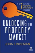
Much of the irregular price-growth of housing is caused by the underlying inflation rate, and it was high inflation that led to the well-touted doubling of house prices every eight years in the 1970s and 1980s. Figure 1.3 (overleaf) demonstrates this correlation, with house prices closely copying the inflation rate, but usually performing slightly better.
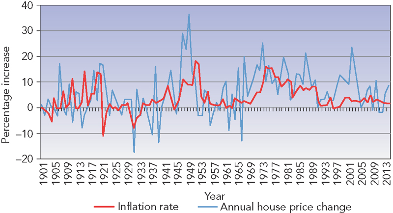
Figure 1.3: house price movements mirror the underlying inflation rate
Source: Australian National Library's online Trove facility; Mitchell Library archives; CPI and IRPI data adapted from Data on Request, Australian Bureau of Statistics.
In fact, the only years when house price-growth significantly exceeded the rate of inflation was during the postwar baby boom years of 1947–50, during the years 1970–73 when the baby boomers purchased their own houses, and then again during 1998–2002 when the children of the baby boomers purchased their homes.
The close correlation between house prices and inflation means that the behaviour of the housing market is actually quite predictable, but only when measured at a national level and only over long periods of time. House price-growth in major cities has consistently averaged about 2 per cent per annum above the underlying inflation rate since 1901, but since the end of the Second World War in 1945 this rate has risen to about 3 per cent per year. The cause of the slightly higher growth rate is due to higher demand for housing in capital cities. Our overseas migration rate has been much higher since the war, and most of these new residents prefer to live in cities such as Sydney and Melbourne, resulting in a higher demand for housing than in regional and rural markets.
High demand for city living is unlikely to change anytime in the foreseeable future, giving us a simple rule of thumb to predict price-growth. Over long periods of time, the rate of house price-growth is likely to average about 3 per cent in capital cities plus the underlying rate of inflation. This means that when the annual rate of inflation averages about 2 per cent, a typical investment property is likely to deliver 5 per cent per annum total growth, even though there might be significant price swings from year to year. That is the best that a buy and hold strategy can offer you, because it is based on the actual long term performance of the housing market. If this were all that housing investment provided you might be tempted to buy shares or even gold instead, but it is the third finding about how the housing market performs over long periods of time that is the most significant of all and demonstrates why property investment has the edge over other forms of investment.
Housing prices change in accordance with supply and demand
Some of the years since 1901 witnessed extremely high house price-growth, and others none at all, but the overall performance of all capital cities tends to even out the booms and the busts. When we drill down to individual capital cities as figure 1.4 (overleaf) shows, each year since 2002–03 has produced a different highest price performer.
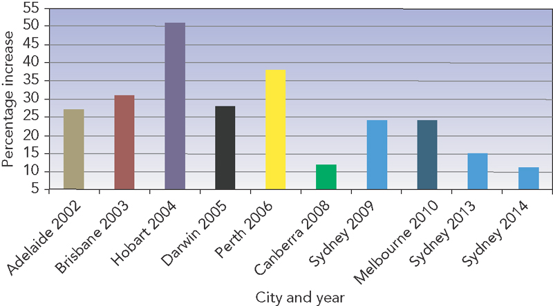
Figure 1.4: every capital city takes its turn as the highest price performer
Source: Australian Bureau of Statistics.
Adelaide's house prices rose by over 25 per cent in 2002 and Brisbane's shot up by more than 30 per cent the next year. Not to be outdone, Hobart's house prices rocketed upwards by 50 per cent the following year. In the next ten years, however, there was little price-growth in any of these three capital cities. Sydney, on the other hand, had virtually no house price-growth from 2003 onwards until 2009, and then was the best performer again in 2013 and 2014. But even including these three best performing years, Sydney's total house price-growth from 2002–14 has averaged only 6 per cent per annum, which is still lower than Brisbane, Adelaide, Perth or Hobart over the same time.
Although the annual price-growth of all capital cities was close to the long-term annual average, you can see that each city performed quite differently. This is because price booms are rare and they don't last longer than a year or two, being caused by a sudden increase in buyer demand combined with a shortage of stock available for purchase. While such growth spurts are sweet for investors, they are also short because the high price rises in themselves dampen demand and buyers look elsewhere. They take place in all types of housing markets, at any time — and just as the growth rates between cities can vary hugely, so can the growth in the suburbs of each city.
Some suburbs may be about to boom while others are falling in price. Past performance won't tell you which suburbs are likely to boom, because the conditions that caused price and rent changes in the past are very likely to be different in future. Housing is a commodity and prices will change according to changes in supply and demand. You would think that this simple truth would end the mystery and misinformation out there once and for all, but it hasn't because the housing market doesn't appear to act that way at all.
Housing behaves differently from other commodities because there are in effect two housing markets. About a quarter of the dwellings that make up the property market are investor-owned rented properties. Rental properties and owner-occupied properties can behave very differently from each other in accordance with the changing relationship of demand and supply for properties in each. Demand for housing can flow into either market, so that when housing finance is tight or costly, rental demand increases and the rental market grows in size and value, while if housing finance is cheap and freely available, buyer demand rises and the renter market declines and rents may fall.
Because most suburbs have a combination of both rented and owner-occupied dwellings, prices may rise while rents will fall in some suburbs, although in others both rents and prices may rise or fall or rents can rise yet prices fall. While each of these markets has its own dynamics of demand, they are connected because households move from one to the other, starting out as renters and then usually becoming buyers and sellers. This means that there needs to be a constant supply of properties for them to purchase in the buyer–seller market, and as they leave the renter market there also needs to be a constant supply of new renting households to keep up the rental demand. If you remember that renter demand controls the renter market, while buyers and sellers control the price market, you can unravel the mysteries of why the market behaves as it does and make some meaningful predictions.
The future will not be the same as the past
Some housing market analysts link the housing market's future performance to intangibles such as unaffordability, or to interest rates; national, state or local economic performance; unemployment; infrastructure development; or even to consumer confidence. No matter which of these dynamics (if any) is right, the facts are that the future of our housing market will be very different to its past. No period in history is exactly like any other, and we continually face climatic, social, economic and financial situations that we have never had to deal with before. Analysing these changes helps us to understand why the housing market has performed in the way that it has, but it also teaches us that relying on the recent past to point the way forward is futile.
The difference between making a prediction and a prophecy is to know just how far into the future we can actually see with some certainty. No-one could have accurately predicted the housing market's performance in 2008–09 without also anticipating the intensity of the Millennium drought and the onset of the Global Financial Crisis, along with the subsequent changes in housing finance lending and overseas migration.
This is why long-term prediction is difficult: even with the benefit of the most accurate prediction methods, the further into the future we attempt to predict, the greater the likelihood of unanticipated events that will throw our forecasts into disarray. No matter how good our explanations, short-term forecasts are likely to be more accurate than long-term ones. Luckily the housing market is on our side, because prices and rents can move substantially in relatively short periods of time, and they do so in accordance with easy-to-understand supply and demand principles.
The secret to unlocking the housing market's future is to understand that housing is a commodity that we buy and sell, just like a car, a boat or even an apple. Yet we don't usually think of housing as a commodity, because we normally don't buy our homes as investments but for other reasons. Home provides us with security and comfort, a place to raise a family or retire to. Another reason that we don't think of housing as a commodity is that it doesn't seem to behave like one. Its behaviour often confounds even the most serious analysts, yet if we rely on facts rather than on fables to forecast the future we find that the market behaves in predictable ways.
The housing market suits all types of investors
Understanding how the housing market works enables you to choose the best type of investment because, just as there are different types of investment outcomes, so there are different types of housing markets that can deliver those results. Some suburbs are suited to active ‘make it happen’ investors who conduct cosmetic or structural renovations for short-term gain, while other areas suit passive ‘let it happen’ investors who engage in flipping and trading. Some investors want high cash flow and others seek suburbs that have boom price potential. There are even localities with few prospects apart from hearsay or gossip that something big is about to happen, where investors speculate on a ‘hope it happens’ basis. Because the housing market is a huge jigsaw puzzle with 10 million properties spread over 15 000 suburbs, we need a simple way of putting the pieces together. This way we can categorise all these suburbs into a few groups that offer similar opportunities, risks and likely performance results.
Figure 1.5 divides the 15 000 suburbs into four distinct groups, each of which offers different outcomes for property investors. These groups are called cash cows, shooting stars, long shots and sleepers. The suburbs in each have certain characteristics in common that identify them, such as:
- types of properties
- types of renters
- price ranges
- location.
Figure 1.5: solving the property investment puzzle
This makes them easy to find and, armed with this knowledge, you will have a much better chance of buying the best possible property in an area where you understand what opportunities are on offer and which hidden dangers may lurk in the background.
Most suburbs are sleepers
Sleeper suburbs form by far the greater number of our capital city and regional town housing markets. This is where median prices and rents move in tune with the overall performance of the market, and the reason this happens is due to the sheer weight of sleeper suburb numbers — it's their rent, price and yield performance that is responsible for the capital city median house and unit price changes we read about. It is therefore essential that investors in such suburbs fully inform themselves about the average performance of the market and the implications for their investments. The key to investment success in sleeper suburbs is being able to read them well enough to pick suburbs for short-term investment just before any price-growth starts, and then sell before it stops.
Some investors get itchy fingers watching the ebb and waiting for the flow of prices in sleeper suburbs, and so they decide to saddle up in search of the elusive long shot suburb where spectacular returns await the more adventurous.
Long shots promise high returns but with high risk
The hope of buying in a town or suburb just before it bursts into spectacular growth is something that appeals to us all. It would truly be like winning a property lottery, because only very few who make investments in long shots ever hit the jackpot. Such investments are based mostly on pure speculation around expectations of increased housing demand in the future, from a new or expanding mine operation, proposed railway line, port or freeway — or from other investors.
Announcements about possible mining or infrastructure development in remote and previously unheralded towns are always accompanied by an increase in house buyers. As a result, the local housing market quickly moves from ‘stressed’ to ‘seller’ conditions, and may even boom. But without any genuine housing demand, the number of profit-taking sellers also rises and prices can quickly reach a tipping point if the number of properties on the market approaches the number of buyers. Within a matter of months, prices are stripped down to where they started and even lower, because the number of potential sellers is now far greater than the number of buyers, even though the total number of buyers and sellers during the entire course of the drama is equal.
These price movements have little to do with land's real value, but are all about speculation. For those of you willing to obtain such rewards, remember that the risks are high as well.
Cash cows offer high rental yield and security
Cash cow suburbs are the holy grail of many investors because they provide high rental yield and price stability driven by a constant supply of renters. Rental yield is a function of both the house price and rental rates, as it is the annual rent from a property expressed as a percentage of the purchase price. Because 2 per cent of a property's value is usually spent each year in maintenance, management and expenses, an investment property whose rental yield also covers the loan interest plus the holding costs is said to be positively geared. This is because it provides net cash flow back to the investor from the rent. The higher the yield, the better the return; and the highest rental yields usually come from three sources:
- Overseas arrivals who move into older, well-established suburbs typified by large ethnic communities and proximity to public transport.
- Emerging households (young people leaving home for the first time) who prefer inner urban medium- and high-density living close to recreational and entertainment areas.
- Reservoirs of permanent renters: low-income households who live in ex–housing commission dwellings and former holiday homes on the fringes of cities and country towns.
Cash cow suburbs suit investors with fairly modest buying price ranges whose aim is positive cash flow along with the security of price-growth over time. The main risks come from over-development, particularly in inner urban unit precincts, and reduction in the migrant intake due to changes in government policy.
It is also important to determine where overseas arrivals are likely to come from in the future, as this will play a large part in choosing locations where these groups prefer to live until they become established and buy homes of their own. The easiest way to find cash cow suburbs is their shared characteristics of high rental yield and rental demand. Out of all the suburbs and towns in Australia, less than half usually have short-term rent growth potential and, of these, just half again have long-term price stability. It's even more difficult to isolate those suburbs where there are properties that can generate a positive cash flow from day one.
The issue that investors have to face is that the suburbs often featuring in high rental yield lists are there for the wrong reasons. Rental yield is the amount of rent received in a year expressed as a percentage of the purchase price, so if prices fall, it pushes the rental yield up. The rental yield may even rise enough for the suburb to feature as a ‘high rental yield’ performer, even though this has been caused by falling prices rather than by rising rents. Indeed, some of these suburbs can have abysmal rental vacancy rates. Yet even though there are only a few hundred cash cow suburbs they are not hard to find, because the percentage of renters is well above the national average, housing prices in the suburb are stable and the rental yield is attractive. If the numbers add up, you may well have found your own cash cow suburb.
Shooting stars provide both high rent and price-growth
When the sleeper, long shot and cash cow suburbs are removed from further consideration we are left with something special: the shooting stars, which are investment areas that have high price-growth potential, high rent-growth forecasts and high rental yield. The number of potential candidates diminishes rapidly as we discard suburbs that don't meet all these criteria. Due to the high risk and performance volatility of mining towns you won't find shooting stars there, nor are they in the attendant dormitory towns, ports and processing centres. The attraction of shooting star suburbs for investors is enhanced by the usually low median buying price, normally far less than the median price for the state as a whole, which leaves plenty of room for price-growth. They tend to be located in areas of high population growth with high rental demand and local housing shortages.
The three dynamics of housing markets
Shooting star, cash cow and long shot suburbs are defined by the households moving into them and whether they rent or buy, creating shortages in the process. These changes are called the dynamics of housing markets, which simply means the causes of price or rent changes. So to identify the individual investment prospects of any suburb, we need to understand its dynamics.
Knowing how the dynamics of any housing market operates will remove a great deal of uncertainty from your property investment decisions because they reveal the reasons why prices and rents are likely to rise or fall. The good news is that there are only three key housing market dynamics that you need to understand and track to make accurate predictions:
- people
- purchasing power
- properties.
The bad news is that they are so little understood that they seem to be secrets, zealously guarded by the few who know their predictive power. Let's uncover these property prediction secrets and discover how to use them — to see:
- how people create housing demand
- why purchasing power turns this demand into rentals or purchases
- how local shortages or surpluses of properties then result in housing price and rent changes.
One of the reasons that these three property prediction secrets are so little understood is that they always work together to create price and rent changes. Relying on just one in isolation, such as high population growth, or the availability of cheap and easy finance, or a local housing shortage, to predict future performance is flawed, yet many property market predictions are made this way. Because such predictions often fail, they may leave us thinking that the housing market behaves erratically or even illogically and that its current performance is no exception. To discover what is causing seemingly illogical market behaviour and what the likely outcome will be, we need to see how the three key dynamics — people, purchasing power and properties — work together.
People create demand for housing
We all need a place to live, so every new household increases our overall housing demand by one. Figure 1.6 shows the annual change in our population that has occurred since Federation in 1901.

Figure 1.6: Australia's population has always been growing
Source: Australian Bureau of Statistics.
The most significant fact is that it has always been growing, even during the darkest years of war, recession or depression. From its lowest annual growth rate of 0.5 per cent in 1944, our population grew by a record 2.7 per cent just a few years later in 1953. Not only has this created a more or less constant shortage of housing, the shortage has been greater in our capital cities, where most of us have preferred to live.
This pressure on housing in capital cities has been worsened by a constant drift to cities by people from the country. In fact, existing households moving from one location to another have a far greater effect on housing markets because every household moving into a suburb increases the demand for a dwelling by one, while at the same time increasing the supply by one in the suburb the household has moved out of. Moreover, the numbers of existing households who move each year is far greater than the numbers of new households, so they have a far bigger impact on local housing markets.
While this movement changes the demand and supply balance wherever it occurs, it is the type of households who are moving into and out of areas that directly affects prices or rents, as well as the number of investors who buy and sell, but don't actually live in the houses or units that they own. Table 1.1 (overleaf) shows the various households who buy and sell properties and the types of housing markets that they create.
Table 1.1: the main types of buyer and seller markets
| Type of market | Total households | Average stay | Typical family types | Location of houses | Location of units |
| First home buyers | 1 000 000 | 4 years | Ex-renters | Outer suburbs | Transport corridors |
| Moving and improving upgraders | 4 000 000 | 10–30 years | Families with children | Established suburbs | Beaches, bays and views |
| Retirees | 1 000 000 | Rest of life | Older households | Coastal towns and retreats | Recreational resorts |
| Renters | There are about 2 500 000 private investor–owned properties as well as about 500 000 government-owned properties, also known as public housing. | ||||
The four main buyer and seller groups are:
- first-home buyers
- people upgrading to a bigger home or a better location
- retirees making their final purchase
- housing market investors.
First home buyers usually buy in the same city where they have been renting, but not the same suburb. They may have been renting an inner urban unit close to recreation and employment, but can only afford to buy an outer suburban house or unit in a growth corridor in a less-than-perfect area. After several years in their first home, most owner-occupiers usually decide it's time to move either to a bigger home in the same location, or to a better location. They hardly ever upgrade to another city because of family, employment and social ties, so the demand they create when they move is concentrated in well-established locations with good facilities and services in the same city and in their purchasing price ranges, which are generally around the median price for the capital city.
After one or two such upgrading moves, the average family does not move again for about 25 years or so, providing the well-established suburbs where they live with the greatest price stability of all types of housing markets. The final move a buyer and seller family makes is when the children have grown up and left and the family home is too big, requires too much maintenance and possibly also represents their greatest asset. The choice of a retirement location is ultimately determined by the nature and location of the new area, the relative purchase price compared to the sale price of the family home and its proximity to the children and grandchildren.
These three types of owner-occupier types of markets make up nearly all of the sleeper suburbs covered earlier in this chapter. So where are the shooting star, long shots and cash cows? They are located in the last group of buyer and seller markets — in those suburbs where investors own most of the properties.
Investors form the second-largest group of buyers and sellers but don't live in their properties. They are motivated purely by profit, can buy and sell without moving and do so more often than other buyers and sellers, but they also create accommodation for renters and so we need to consider the housing markets where they buy and sell properties differently to owner-occupier markets — as the four types of renter markets shown in Table 1.2.
Table 1.2: the main types of renter markets
| Type of market | Total households | Average stay | Typical family types | Location of houses | Location of units |
| Permanent private renters | 500 000 | Permanently | Low incomes, single-parent families | Ex–housing commission, ex–holiday homes, rural outskirts | Older unit enclaves |
| Overseas arrivals | 1 500 000 | 4 years | Permanent arrivals from overseas | Ethnic enclaves in affordable rental suburbs | Ethnic enclaves near services and facilities |
| New households | 600 000 | 2 years | Young households leaving home | Established inner suburbs | Inner urban areas with services and facilities |
| Opportunity seekers | 400 000 | 1 year or less | Singles, groups | Mining, tourist towns, dormitory towns | Mining, tourist towns, dormitory towns |
Permanent private renter markets offer high yields and low risk and many form cash cow suburbs, but because of their low prices the opportunity for capital growth is diminished. Temporary renter markets cross a wide spectrum of prices and offer great variations in growth potential and rental yield as well as presenting varying degrees of risk depending entirely on the types of renters moving into and out of an area. They may be inner urban high rise precincts favoured by new younger households looking for quality lifestyle, modern facilities and proximity to entertainment and employment, or older suburbs where recent arrivals from overseas can find rental accommodation near ethnically similar neighbours, schools, shops and religious institutions. They may be new mining towns or tourist resorts where the people seeking employment are renters with no intention to buy a property, because they will only stay while the opportunities last.
Every type of housing market performs differently as time goes by — sometimes first home buyers lead a growth charge, at other times it may be retirees. Investors may buy into high rental demand areas such as mining towns or inner urban unit precincts and create growth and then depart again if rental demand dries up. On the other hand, there are some regions and localities where populations are falling. Decreasing populations in Australia are caused by people moving to another state, or another area within the same state; such movements may be hidden by commonly used statistics. Figure 1.7 shows that while Tasmania's two largest cities, Hobart and Launceston, maintain a healthy population growth rate, the rest of the state is falling in population.

Figure 1.7: Tasmania's annual rural population drain
Source: Australian Bureau of Statistics.
Thousands of younger Tasmanians leave the state each year, seeking better employment, educational, recreational and social opportunities. This is causing a population decline in rural Tasmania that is hidden because, at the same time, an almost equal number of older people move from the mainland looking for affordable retirement options or lifestyle changes. Although young people leave empty nests behind rather than empty houses and interstate arrivals need housing immediately, the effect is more dramatic on the housing market in rural areas because the younger people leaving are not being replaced.
Tasmanian rural towns such as Zeehan, Roseberry and Queenstown often feature in free reports because they periodically generate the highest rental yields of any Australian housing market, but be warned: younger people are deserting those towns, leaving behind ageing populations, high rental vacancies, falling house prices and a rising number of derelict and deserted homes. This is why you need to understand the type of housing market that predominates in any area where you may be thinking of buying an investment property and how the demand is changing — that is, what types of households are moving in and which are leaving — as this helps you to estimate whether prices and rents may change.
Purchasing power creates buyers or renters
When new households are formed or move from one area to another, they will either rent or purchase a property. First home buyers borrow as much as they can afford in order to live in an area and type of dwelling that meets their needs, but there is usually some trade-off involved, because the amount they can borrow as well as the repayment commitments are limited by lenders. Upgraders will have some equity, may have higher incomes and the interest rate may have shifted in their favour over time, so they can afford to move to a bigger dwelling, or a better area by increasing the borrowed amount. Over time, they may even be able to use their equity to reduce the amount financed and still be able to upgrade. In fact, most retirees will use their equity to buy a suitable retirement home, retire their debts and still have a nest egg left over for the future. Investors will either buy for capital growth, in which case they will borrow most of the purchase price to leverage their investment, or buy for cash flow, in which case they will borrow as little as possible and provide rental accommodation.
Just as not all buyers need finance, not all renters intend to buy. The crucial point here is that most aspiring home buyers will purchase their first home in a different suburb to where they live. A young couple renting a high-rise unit in inner Sydney or Melbourne is highly likely to buy their first home in an affordable outer suburb, where they intend to start or expand their family. Overseas arrivals will rent in affordable middle distance suburbs until they are sufficiently well settled to buy their own home, and this is likely to be a statement of their successful establishment in a new country. This means that as new households and overseas arrivals change from renters to purchasers, they reduce the demand for rentals in the suburbs they leave and increase the demand for purchased homes in the areas they move to. There are, however, two groups of renters whose primary aim is not to purchase a home — at least not directly. They are the 500 000 permanently renting households on low incomes in ex–housing commission and holiday home areas. Although they are located on the outskirts of our major cities, they may also rent older, less desirable units in urban areas as well as older houses in country towns. The other group are the opportunity-seeking renters, looking for high income employment in mining towns, casual employment and holiday lifestyles in tourist resorts or education in university towns. Although they have no immediate intention to purchase homes of their own, and certainly not in the towns where they are renting, they are a highly mobile group of renters and control the fortunes of investors who buy properties in such areas. It is their demand for accommodation or lack of it that sets the boom or bust sequence in motion.
We have seen that the continual rise in our population has led to a more or less constant shortage of housing, especially in capital cities, but this does not automatically lead to a rise in housing prices, because some households cannot afford to buy a home, or don't want to. Figure 1.8 (overleaf) shows how this has played out since 1901, with rents rising strongly during periods such as the Great Depression in the early 1930s, when housing finance was simply not available, or during the early 1950s when large numbers of postwar overseas arrivals were forced to rent for several years until they were settled.

Figure 1.8: either house prices or rents have always been rising
Source: Australian National Library's online Trove facility; Mitchell Library archives.
At other times, such as the immediate postwar years of 1919 to 1921 and 1946 to 1951, house prices rose strongly as soldiers arrived back home from years of service, keen to start families and buy homes with generous government war service home loan assistance. Figure 1.8 shows how rents actually fell in those years as new households left rental accommodation to move into new suburban homes they were buying.
Demand and supply changes in properties lead to shortages or surpluses
Because of the issues with collecting timely population movement data and housing finance data for areas smaller than capital cities and states, some predictive systems resort to other methods of trying to estimate demand, such as time on market, vendor discounting, rental yield, or even online search interest ratios, none of which may be accurate or even appropriate. How then can we measure the number of people moving into or out of a suburb and determine whether they are renters or owners?
We can simply do this by measuring the effect they have on the housing market. If people move into a suburb and buy properties, the numbers of property sales rise and the number of properties for sale goes down. If they move out, the number of property sales falls but the number of properties for sale goes up. This will only lead to a rise in property prices if the number of potential buyers climbs above the number of properties for sale. In other words, if there is a shortage of properties available for purchase, and potential purchasers start to compete with each other to buy. So if the number of buyers rises but there are plenty of properties for sale on the market, prices will not go up. This is the law of supply and demand and it works in the property market just as it does with any other commodity. It also means that a fall in sales will not necessarily lead to a fall in price, unless the number of properties for sale, that is the supply, is more than the demand.
Some movers don't buy; they rent. But the same rules apply, in that if the number of potential renters rises above the number of rental vacancies, rents are likely to rise as prospective tenants compete with each other. On the other hand, if rental demand drops and results in a rise in rental vacancies, investors trying to let their properties will compete with each for tenants and rents will fall.
It would seem, then, that all we have to do is determine where households are likely to move in future, and whether they are likely to purchase or rent, and we can accurately predict housing demand in those areas. We can estimate whether this could lead to a shortage or surplus of properties and even forecast the probable changes in prices and rents.
In fact there are some predictive systems in the market that attempt just this task, but there are some fundamental issues with this approach. First, housing data such as the number of renters, number of properties, even number of residents in a suburb is only gathered every five years by the Bureau of Statistics in the Census of Population and Housing. More frequent updates are trend estimates and not provided at suburb level, so the data being used in these predictive systems is not current, and could be up to six years out of date. Second, the only effective ‘rent or buy’ statistic is Housing Finance, but although this is provided monthly by the Bureau of Statistics, it does not drill down below capital city and states, so we don't know where owner-occupiers or investors are buying properties. In addition, housing finance data doesn't give us any information at all about purchasers who don't need finance, such as retirees.
It is as if there are two housing markets in any suburb: one for renters and another for buyers and sellers. They can behave very differently, but it will always be the supply and demand situation in each that determines whether rents or prices will rise or fall.
![]()
This first key has unlocked the mysteries of how the housing market works and demonstrated the importance of looking forward rather than backwards. We have solved the investor puzzle and revealed the three dynamics of the housing market, to show you how they lead to price and rent changes. The next key shows you how to easily measure the current state of any housing market and predict its likely price and rent performance.