
The Old and the New
Array formulas have a reputation – and it’s not a particularly good one. For many spreadsheet users, they’re Excel’s equivalent of a dark alley at 3 in the morning; one just doesn’t go there.
Why not? Possibly because array formulas ask the user to think of, and work with, ranges in a way that displaces them from their comfort zone. Every spreadsheet formula works with ranges, of course, but array formulas – both the earlier and the newer dynamic-array kind – subject the values to a different kind of collective treatment.
=SUM(LEN(A1:A3))
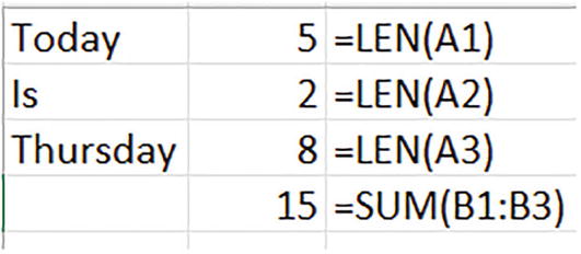
A table of 2 columns and 4 rows. The data in the last column and rows have the formula for LEN and SUM on the right.
Going to great lengths: adding the lengths of words individually
=SUM(A1:A1000)
That task, then, would require 1001 formulas.
While of course these results will be correct, the array alternative could engineer the same outcomes with exactly one formula. If you needed to calculate the total lengths of 100,000 words inundating the A column, you’d have to direct 100,001 formulas at them. The array formula count? Again, one.
=LEN(A1:A3)
And you’d then surround, or wrap, that formula with the SUM function.
This array formula carries out two operations – the cell-by-cell length calculations as well as their overall sum – and again, within the space of one formula. It’s this way of thinking, in which the formula is made to multitask with multiple values, that may be new to you, but a bit of reflection about the array process along with some directed practice will serve you well.
=LEN(A1:A3)
freed of SUM, will release its results into multiple cells. It’s as if the SUM function locks its data inside the formula, forcing a single aggregated result into a single cell.
An Important Reminder
=SUM(LEN(A1:A3))
=LEN(A1:A3)
can only be successfully written in Excel 365 or later, because it will lodge its results in multiple cells.
Remembrance of Keystrokes Past
And those reminders recall another reason why so many Excel users crossed the street when they saw an array formula coming. If a user mustered the courage to actually write one of them in the bygone, pre-365 days, the array formula was instated in its cell not via a simple tap of the Enter key, but by banging out a fearsome triad of keystrokes instead: Ctrl-Shift-Enter.
=LEN(A1)
=LEN(A1:A3)
But Ctrl-Shift-Enter forced, or as the geeks like to put it, coerced, formulas to suppress their just-one-result instinct and make room for multiple results instead – even if for first-generation array formulas those results were confined to the formulas themselves. That process is called lifting, and is integral to array formulas; but more to the point, lifting now serves as Excel’s default formula capability. In any case, we’ll have more to say about lifting later.
{=SUM(LEN(A1:A3))}
The brackets, those squiggly formations we’ve seen attaching to arrays in the inner recesses of formulas, here showed up in actual formulas in their cells, doubtless triggering the same question in the minds of countless Excel users: what in the world are those?
That, too, was a good question, once upon a time. But not to worry, with the advent of dynamic arrays, both Ctrl-Shift-Enter and the brackets flanking array formulas have been abolished, and if you never knew about them to begin with, you’re in luck – there’s nothing for you to unlearn. They’re gone. Nowadays, every Excel formula, array or otherwise, springs into action with Enter and nothing more. As for the brackets, more need be said, but rest assured: you won’t see them clamped around formulas in their cells.
A handful of pre-365 formulas, most notably SUMPRODUCT, were empowered with native array formula status and so only required the user to press the Enter key. But even SUMPRODUCT could still only deliver its result to a single cell.
Back to the Basics
=FORMULATEXT(C1:C4)
Press Enter, and the deed is done. One formula, multiple instances of FORMULATEXT (again, “spilling”), and no brackets. Just remember that you can’t write this one in earlier versions of Excel.
And that spilled range bears a closer look. We’ve written the formula in C1, and of course a click on that cell will disclose what we’ve written there. But click on C2 and the same formula will appear, but dimly – in a kind of shadow emanation of the original. You won’t be able to delete C2, or any cell that’s been spilled by the source formula. Delete C1 – the cell featuring the actual formula, on the other hand – and the entire spill range will vanish.

A table with 4 rows. The values read John, Paul, George, and Ringo.
A quartet of values
=Beatles
anywhere in the worksheet (or any other sheet in the workbook, by default), and immediately spill those names down its column.
That’s pure dynamic arraying at work, and that kind of range can offer to the thoughtful user more than gimmickry. A teacher could list all her student names in a range and call it Class, and by typing =Class anywhere else in the workbook could immediately summon all the names for grading, attendance, or any other administrative purpose. A work supervisor could do the same with a staff roster; type the range name, and the roster appears.
And by way of review of our discussion in Chapter 1, be reminded that writing =Beatles in pre-365 Excel and tapping Enter would result in “John” – and only John.
Now for the record, a multi-cell workaround of sorts did avail itself to the pre-365 generation. If I were to select four cells first, proceed to click in the formula bar and enter =Beatles, and then enter Ctrl-Shift-Enter, the names of each of the Fab Four would indeed make a place for themselves, one to a cell. But that’s a tricky – and inefficient – ask.
The One-Formula Grader

A table of 3 columns and 10 rows. The column headers are quest dot, answer key, and student. The values are given for all 10 rows.
Multi-cell multiple choice exam
The answer key occupies B4:B13, alongside the student’s replies in C4:C13. The obvious objective: to determine the student’s overall grade.
=IF(C4=B4,1,0)

A table of 4 columns and 11 rows. The column headers are quest dot, answer key, student, and blank. The values are given for all 10 rows. The blank column has the formula IF and SUM on the right side of the values in the final row.
Assessing the assessment: calculating the student’s grade
(We could go further and divide the correct-answer total by the number of exam questions, returning a score of 60%; but that step isn’t necessary for our demo purposes.)
=SUM(IF(B4:B13=C4:C13,1,0))

A screenshot of the function arguments window. It has input boxes for the options, logical test, value if true, and value if false. An arrow points to the equal to value at the bottom.
Rights and wrongs: the test answers gathered in an array
We’ve just encountered another instance of lifting – this time a special case called pairwise lifting, in which each pair of values sprawled across their rows are compared, as the formula spills its results down the D column. Our single IF formula has been made to tear up its job description and evaluate data in a range of cells; and those 1’s and 0’s – all housed in the inner sanctum of the formula – total 6, the student score.
=IF(B4:B13=C4:C13,1,0)

A table of 4 columns and 10 rows. The column headers are quest dot, answer key, student, and blank. The blank column has the formula IF on the right side of the first cell.
Going solo; a single IF statement calculates each grade.
Shades of LEN(A1:A3). Here too, the IF statement – minus SUM – assigns its 1’s and 0’s alongside each student answer. Again: one formula that disgorges multiple, spilled results in their cells – an outcome only possible in Excel 365 and beyond.
The Return of the Brackets

A table of 7 columns and 10 rows. The column headers are name, s o c, Philosophy, Political Science, Art, Physics, and Chemistry. The values are given in each row.
Six subjects in search of a formula
Once again, we’re asking a formula to step out of character – the venerable VLOOKUP had been genetically tweaked to look up the values in a single column, and now we want it to track down the values in two columns at the same time – and compute their average, besides. What would that VLOOKUP look like?
=AVERAGE(VLOOKUP(I9,All,{2,5}))
And we learn that Jane averaged 69 for the soc and art exams.
But there are those brackets again – the ones you thought had been permanently banished from array formulas, and tucked irretrievably into the archives. But those brackets were of the automatic variety, the ones that leaped into a cell whenever you put the finishing touches on an old-school array formula via the now-obsolete Ctrl-Shift-Enter. These brackets are user-selected and user-typed, and they throw an actual, on-the-fly array smack-dab into a formula. The values between the brackets are called array constants, so named because they’re hard-coded, or simply typed. But don’t get the wrong idea – the constants aren’t inert text: here they serve to quantify the column numbers you select, and so in our case they tell VLOOKUP to search for data in columns 2 and 5. If we had entered {2,5,7}, the VLOOKUP would go ahead and compute Jane’s average for soc, art, and chem: 64.67. The bottom line is this: the array constants force VLOOKUP to undertake a multi-column search for values. And once again, because all this derring-do yields a one-celled answer – the test average – our formula can be written in previous versions of Excel, but remember that if that’s where you find yourself, you’ll need to ratify the formula with Ctrl-Shift-Enter.
=VLOOKUP(I9,All,{2,5,7})
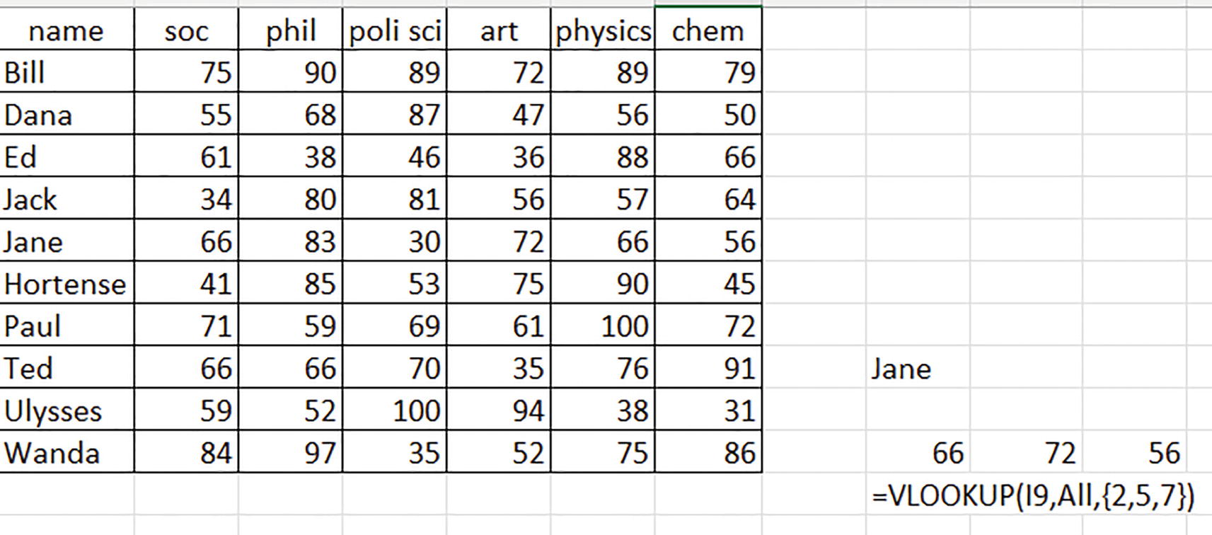
A table of 7 columns and 10 rows with values. The column headers are name, s o c, Philosophy, Political Science, Art, Physics, and Chemistry. The formula V LOOKUP is given on the bottom right for the entry Jane and its values.
It’s all academic: Jane’s scores in soc, art, and chem
And again, that output confirms the multi-cell capability of dynamic array formulas. You’re doubtless getting the idea.
Getting Re-oriented
But that last formula raises a new question. You’ll note the horizontal alignment of Jane’s three scores; but why do they proceed across a row, and not down a column instead?
{2,5,7}
=VLOOKUP(I9,All,{2;5;7})
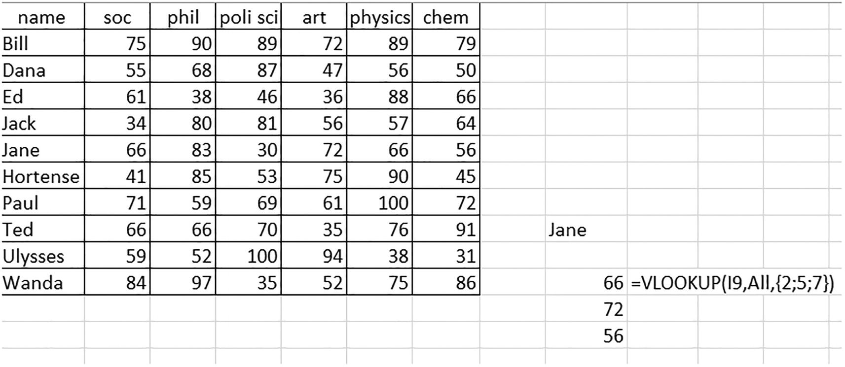
A table of 7 columns and 10 rows with values. The column headers are name, s o c, Philosophy, Political Science, Art, Physics, and Chemistry. The formula V LOOKUP is given on the bottom right beside the value 66 of the entry Jane.
Downward trend: Jane’s scores in vertical orientation
More of the Same
=LARGE(A1:A100,3)
=LARGE(A1:A100,{1,2,3})
Again, the formula would roll out three results, one per cell; and because the array is comma-separated, they’d spill across a row.
But a Workaround Is Available
But if you just don’t like those pesky brackets, here’s a surprisingly obscure but easy workaround that can make your array formulas bracket-free:
=VLOOKUP(I9,All,I10:K10)
That new take achieves the same results, sans brackets; and if you want to change the column numbers to be looked up without editing the formula directly, just enter a different number somewhere in I10:K10.
Summing Up
We’ve devoted this chapter to a review of some of the essential features of first-generation array formulas, the new complement of dynamic array formulas, and what distinguishes one from the other. Note that – and again this is important – our review has run through its paces without having called upon any of the new dynamic array functions. That purposeful omission is a reminder that Microsoft’s grease monkeys have installed the dynamic array engine into most of Excel’s functions, and not merely the new ones. In the next chapter we get a bit further under the hood and explore some of the additional mechanics of the engine. No overalls required, though.