
What’s Unique About It?

A table has 5 columns and 15 rows. The column headers are country, salesperson, order date, order I D, and order amount.
Selling point: Salesperson data to be subject to the UNIQUE function
The problem, of course, is the recurring appearances of each salesperson’s name in the field – because we want to view each name exactly once.
=UNIQUE(Salesperson)

A table has 3 columns and 9 rows. The function involved is, equals unique (sales person) and the name Buchanan in column 2, row 1 is highlighted.
One time only: each salesperson listed uniquely
Bravo – Excel users have been looking for that kind of performance for a long time.
And if you redefine the dataset as a table and introduce new names to the Salesperson field, UNIQUE will see to it that their names will automatically appear in its result.
=COUNTA(UNIQUE(Salesperson))
=SORT(UNIQUE(Salesperson))
will again return the salesperson names uniquely, but this time in alphabetical order (SORT and SORTBY will make their official appearance in the next chapter).
How It Works
=UNIQUE(range/array,by column,exactly once)
The “range/array” term simply identifies the data to be impacted by the function, recognizing that, as a terminological matter, one person’s range may be another’s array. Here, range and array are in effect equivalent.

A table has 1 column and 1 row. The row entries from left to right are Jane, Ted, Mark, Ted, and Alice.
Getting re-oriented; finding unique names in a horizontal range
=UNIQUE(B7:F7,1)
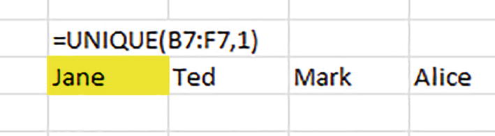
A table has 4 columns and 3 rows. The name Jane in column 1, row 2 is highlighted and the function involved is, equals unique (B 7 colon F 7, 1).
Something’s missing: only unique names returned
Note that, unlike SEQUENCE, both vertical and horizontal ranges are referenced by UNIQUE in the first argument. It’s the optional 1 that orders the formula to recognize the range as a horizontal one (you can also enter the word TRUE in lieu of the value 1).
=UNIQUE(B7:F7,1,1)
will yield Jane, Mark, Alice (again the 1 associated with the third argument can also be replaced by the term TRUE).
While you may be hard-pressed to dream up a real-world use for the exactly once alternative, here’s a couple of possibilities. If you needed to search a list of names for typos, the exactly once option could – could – be of some service. If you had mistakenly keyed in Peacock once in the Salesperson field, UNIQUE’s third argument would find it – but of course if I had committed the same error multiple times, it would not.
You could also apply the exactly once argument to, say, a list of student names in which each name is to be entered a solitary time. Running UNIQUE with the exactly once argument would then simply duplicate the entire list – but would exclude any name inadvertently entered twice.
UNIQUE Stretching Across Multiple Fields
=UNIQUE(Country:Salesperson)

A table has 2 columns and 14 rows. The country France in column 1, row 1 is highlighted and the function involved is, equals unique (country colon salesperson).
Internationally unique: each salesperson is matched to every country in which he/she works
(Again, these data can be sorted, and you’d probably want to do just that; but the how-to’s of sorting will be reserved for the next chapter.)
The formula works by deploying the semicolon to link the adjoining Country and Salespersons fields, building a kind of meta-field which, understood in cell reference terms, reads A2:B799. And UNIQUE then proceeds to dispatch every unique combination of Country and Salesperson to the spill range.
=UNIQUE(first field:third field)
That expression would span the three fields.
Distant Fields

A table has 5 columns and 15 rows. The column headers are country, order date, salesperson, order I D, and order amount.
Faraway countries: the Country and Salespersons fields are separated by a third field
Given that scenario, the footwork for gleaning UNIQUEs for Country and Salesperson gets a little fancier. We need to lace on the INDEX function, a classic spreadsheet tool that, like so many other entrenched functions, has undergone a major dynamic-array renovation.

A table has 7 columns and 11 rows. The column headers are name, s o c, phil, poli sci, art, physics, and chem.
Those grades, again
=INDEX(A1:G11,3,4)
would alight on 87, the grade residing in the range’s third row and fourth column. But now INDEX has been invested with a new aptitude, an important one – for marking and carving out whole ranges. And here, in our case of the Country and Salesperson fields distanced from one another by a third, intervening field, we want INDEX to wrench Country and Salesperson from their current columns and set them down in a new, impromptu dataset consisting of just those two columns/fields; and once they’ve been reunited, we can run a UNIQUE with the Country:Salesperson pairing we’ve already seen.
=INDEX(A1:C800,SEQUENCE(ROWS(A1:C800)),{1,3})
And then we wrap UNIQUE around it all.
Now obviously that formula calls for some explaining, even as it reaches back to some familiar elements (remember that we’re now working with the dataset filling the second, Non-adjacent UNIQUE sheet).
First, the A1:C800 recognizes our need for nothing but the first and third columns in the range, stationed in A and C – the columns storing Country and Salesperson data. We aren’t interested in the data in columns D and E, and as such we can exclude them from the initial range reference. But we also need to exclude column B, the field recording the Order Dates – because failing to eject the data in B will result in a UNIQUE that delivers the unique combinations of all three columns – A, B, and C.
=INDEX(A1:C800,800,{1,3}))
then only row 800 would have been returned.
And as for the bracketed array reference posted to INDEX’s column argument, that entry is familiar too; here it selects the first and third columns in the range – the ones featuring the data we want.
=UNIQUE(INDEX(A1:C800,SEQUENCE(ROWS(A1:C800)),{1,3}))
And that expression should bring about precisely the same outcomes we see in Figure 5.5.
An alternative to the above exercise will be offered in the chapter on the brand new CHOOSECOLS function.
It’s Starting to Add Up
UNIQUE’s penchant for grabbing single instances of values or text in a range can be put to highly efficient use to aggregate data by a variable, or variables. To exemplify that abstract pronouncement with a real-world case, suppose we simply want to determine how much money each salesperson earned (we’re returning to the first sheet in the UNIQUE file). Is that something a pivot table can do? Yep, but the dynamic duo of UNIQUE and the old-school SUMIF (or SUMIFS) can craft a result that can immediately recalculate new data, as well as incorporate new records added to the source data.
=SUMIF(Salesperson,G4#,Order_Amount)

A table has 7 columns and 9 rows. 2 functions of unique and sum are involved in row 1. The entry Buchanan, 70161 point 3 9 in columns 2 and 3 of row 1 are highlighted.
Selling point: UNIQUE supplies the criteria for SUMIF
Note the G4# denoting the cell in which UNIQUE is emplaced, and which serves as the SUMIF criterion.
=TRANSPOSE(UNIQUE(Country))

A table has 6 columns and 11 rows. 2 functions are involved in row 1 and row 3. The country France in column 3, row 2, and the name Buchanan in column 2 row 3 are highlighted.
Matrix in the making: Salesperson and Country in a pivot table impression
=SUMIFS(Order_Amount,Salesperson,G4#,Country,H3#)

A table has 11 columns and 11 rows. 2 functions are involved in rows 1 and 3. The country France in column 3, row 2, and the Buchanan, 27161.35 in columns 2 and 3 of row 3 are highlighted.
Having a field day: Sales totals by the Salesperson and Country fields
And again, any new Salesperson and/or Country names we add to the dataset will find their places in the above results, once we remake the dataset into a table. But because our formula references the Salesperson and Country in dynamic array terms, no formula rewrite would be necessary.
And yes, the above shot bears a striking resemblance to a pivot table; and indeed, dynamic arrays can recreate the number-crunching might of the tables, at least in part (though not completely), and with the advantage of immediately recalculating any new records written to the source data. And that leaves you with one more spreadsheet design decision to make: dynamic arrays or pivot table? Something new to think about.
Up Next
Now that we’ve concluded our introduction to the UNIQUE function, we can move on to a pair of related dynamic array functions you’ll definitely want to learn and master – SORT and SORTBY.