
Good question. That term – array – has secured a foothold in all sorts of computing vocabularies and has made a series of guest appearances in the dictionaries of other scientific domains as well. But while that’s all very nice, you want to know what arrays mean for the Excel user, and how that understanding can add value – quite a bit of value – to your work with spreadsheets.
A Working Definition
Defining spreadsheet arrays is an assignment that brings with it bad news and good news. The bad news is that definitions of spreadsheet arrays vary. It seems, for example, that some writers all but equate the terms range and array. Indeed – a Microsoft website asserts that “You can think of an array as a row or column of values, or a combination of rows and columns of values,” and that sure sounds like a range to me, and leaves me none the wiser; and a Google site describes array in almost the same terms. But because “range” seems so often to be twinned with “array,” we can ask the obvious question: Why then do we need both of them? And just to make sure you’re paying attention, Excel sometimes trots out “vector,” too.
Indeed, Excel savant Liam Bastick (https://www.accountingweb.co.uk/tech/excel/xlookup-and-xmatch-two-new-x-men-for-excel) states that “An array is a collection of cells consisting of at least two rows and at least two columns,” while maintaining that a vector “is a collection of cells across just one row…or down just one column…” Hmmm.
On the other hand, Mike Girvin, author of the near-legendary tome on array formulas Ctrl-Shift-Enter (a volume that has since slipped into near-obsolescence, though the significance of its title will become clearer as we proceed), goes small and calls an array “a collection of two or more items.” I can’t say that I’m edified. And for the late spreadsheet master Chip Pearson, an array is a series of values (http://www.cpearson.com/excel/ArrayFormulas.aspx), but you’re getting the idea.
But time for the good news: Confusion notwithstanding, none of this will stand in the way of your ability to master array formulas. Once you get up and running with the formulas, you’ll be able to relegate the definitional details to mere barroom debate – though if you can track down a bar in which the regulars actually argue about array formulas, please take me there; the next round will be on me.

A screenshot of a function arguments window. The heading at the top is titled sum. Values can be entered for number 1 and number 2. Value in number 1 reads A 1 colon A 3.
Face to face with an array
You’re looking at an array – our values 1, 2, and 3, surrounded by the hallmark brackets that accompany an array expression. The sum itself in the lower reaches of the screenshot – 6 – is bracket-free, because among other things an array must comprise at least two values (but more about that later). And had I replaced SUM with an AVERAGE, or MAX, or COUNT function and proceeded to tick the fx button again, we’d discover that the resulting array would appear precisely as we see it above – {1,2,3}.
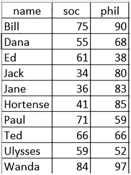
A table of 3 columns and 10 rows. The column headers are name, Sociology, and Philosophy. The row entries are as follows. Row 1: Bill, 75, 90. Row 2: Dana, 55, 68. Row 3: Ed, 61, 38.
Testing, testing: student exam grades to be looked up
After entering any student’s name in I1 and writing a VLOOKUP formula in I3
=VLOOKUP(I1,A1:C11,3,0)

A screenshot of a function arguments window. The heading at the top is titled V LOOKUP. Values can be entered for lookup value, table array, col index num, and range lookup.
Another array, this one produced by a VLOOKUP formula
Here we encounter a subtle difference from the array captured by our SUM example. Look closely, and you’ll note the semicolon that separates the entries “phil” and “Bill,” as well as “90” and “Dana.” That bit of punctuation signals that both “Bill” and “Dana” appear in new rows in what Microsoft here insists on calling the table array (I told you definitions vary), i.e., “Bill” immediately follows “phil” in the array, but appears in the next row in the worksheet (review Figure 1-2). We’ve thus learned a pair of rules about array notation: a comma interposed between array values means they share the same row, while a semicolon indicates that the values break at the semicolon and swing down into a new row in the worksheet – kind of an array word wrap.
Now for Something Different
But in both of our cases – SUM and VLOOKUP – we’ve seen that the formulas have simply grabbed the values from their respective cells in the worksheet and remade them into arrays, readying them for whatever function on which the user decides. But – and this is a big but – sometimes an array consists of values that haven’t been drawn from the spreadsheet, but have been produced by the formula itself.
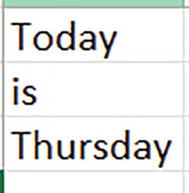
A picture depicts 3 words to form a sentence which is, Today is Thursday.
Cast of characters: words ready for a character count
=SUM(LEN(A1:A3))

A screenshot of a function arguments window. The heading at the top is titled sum. Values can be entered for number 1 and number 2. Value in number 1 reads L E N left parenthesis A 1 colon A 3 right parenthesis.
Three little words: the character count for each word in the range
Unlike our previous examples, the values 5, 2, and 8 in the preceding array appear nowhere in the worksheet; they represent the individual character counts of the three words in our range – and they’ve been calculated by, and restricted to, the formula only.
What we’ve viewing here is an array formula, so called because the formula itself has generated the array. While it’s true, of course, that our SUM and VLOOKUP illustrations also exhibit arrays, we’ve seen that those formulas simply reproduced the data in the worksheet and tossed them into the formulas. Here, the formula builds the array internally, and that’s what we mean by an array formula: a formula that realizes multiple results – here, the 5, 2, and the 8.
What We Mean – and What We Don’t Mean
Note again, on the other hand, that the bottom-line character count in the formula above – 15 – isn’t deemed an array. To restate an earlier point, arrays consist of multiple values. Here, it’s rather the intermediate results, the three character counts, that bind themselves into the array.
And don’t confuse multiple results with multiple calculations. Is it possible, for example, to add a million values with the SUM function? It sure is. Remember that an Excel worksheet hands the user more than 17 billion cells to play with, so summing a paltry million of them is a walk in the park. And it’s true – that formula would have to perform 999,999 calculations, factoring each successive cell value into the result. But that massive process will nevertheless leave us with but one result – the overall total, deposited into one cell.
But an array formula cooks up a batch of individual, stand-alone results, again in our character-count case 5, 2, and 8. That trio of values sits side by side in the waiting room of the formula until some finalizing action – in our case SUM – parachutes the total of 15 into a single cell. But the three distinct results came first, and they came from the formula.
=AVERAGE(LEN(A1:A3))
in which case its result – 5 – will again find its way into its cell. But here too, the average is derived from the array that’s been manufactured by the formula: 5, 2, and 8.
Dave Bruns’ treatment (https://exceljet.net/glossary/array) of “array” verges close to the view advanced here.
Introducing…Dynamic Arrays
Now for the next big point. The two array formulas we’ve introduced – the ones computing the sum of the characters of three words and the average character-per-word – are the kind that can in fact be written in any version of Excel. And that raises an important introductory point. While you may be new to array formulas, array formulas aren’t new to Excel; they’ve occupied a musty, seldom-visited corner in Excel’s storeroom of tools for many years, even if a great many Excel users have been afraid to poke around that corner.
But with the rollout of Office 365 came a radical new development. The way in which array formulas – now labeled dynamic arrays – are written was dramatically retooled and accompanied, you’ll be happy to know, by a significant boost in their ease of use.
So What’s New?
=LEN(A1:A3)
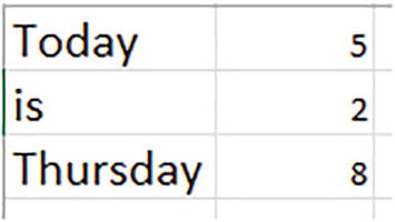
A table of 2 columns and 3 rows. The row entries are as follows. Row 1: today, 5. Row 2: is, 2. Row 3: Thursday, 8.
Character count, this time word by word
=LEN(A1:A1000)
would have done just that. And that’s new for Excel. Try the above formulas in a pre-365 version of the application, and you’ll discover you can’t get there from here. Rather, what you will discover, for example, is that writing =LEN(A1:A3) in cell B1 in the older versions will dispatch only one result – 5 – to B1, for example, the length of the word in A1. That’s because formulas in pre-365 Excel were incapable of depositing multiple results in multiple cells, a shortcoming called implicit intersection about which we’ll learn a bit more later.
The one-formula/multi-cell capability of dynamic arrays is new – and big. It greatly streamlines the formula writing process and, with a bit of imagination, empowers the user to productively apply arrays across an enormous swath of data-manipulating tasks, as we hope to demonstrate.
And so to summarize the plot thus far: While by definition, all array formulas can turn out multiple results, dynamic array formulas can transmit those results to cells in the worksheet, through a process Excel calls spilling.
Moreover, if the range(s) referenced by a dynamic array formula changes, the number of cells that spills – that is, the new result of the now-rewritten formula – will also immediately change. And that’s what’s dynamic about them. And don’t worry: plenty of examples are to follow.
And to further these ends, Excel has brought out a fleet of dynamic array functions poised to supercharge your formulas with that multi-cell firepower – and they’re pretty easy to write, too. In fact, two batches of the new functions have been issued, and we mean to look at them all here – even if you don’t yet have all of them.
And while it’s true that much of this book is devoted to the new functions, precisely because they’re new, don’t let the new ones distract you from the larger point – namely, that nearly all of Excel’s functions – for example, the old reliables like SUM, AVERAGE, VLOOKUP, MATCH, SEARCH, and many more – have been vested with dynamic array clout, too. On the one hand, it isn’t our intention to expound the hundreds of pre-365 formulas in detail – that’s for a different kind of book – but again we want to indicate that these too have been equipped with dynamic array functionality (for a directory of all of Excel’s functions, less the newest ones just announced, look here).
This book, then, isn’t only about the new tools enlarging Excel’s inventory; it’s really about Excel, and how it’s changed, and how it’ll change the way you work.
Some Points to Bear in Mind
Before we begin to describe the workings of dynamic array formulas, let’s offer a few more preliminaries. First, this book can’t hope or presume to tell you everything there is to know about dynamic arrays. After all, given their immense potential, I’m not sure that objective is even possible, and even if it was it would call for a book so enormous you wouldn’t want to read it, and I wouldn’t want to write it. As every halfway-experienced Excel user knows, the same spreadsheet task very often lends itself to multiple approaches, and so the techniques called upon here may well not be the only one.
Second, you’ll note that most of the screen shots reveal the formulas that gave rise to the results captured in the shots. They appear courtesy of the most useful FORMULATEXT function, but these of course won’t automatically materialize on your sheet if you’re clicking along with me.
And finally, it’s acknowledged that the examples placed before you here aren’t necessarily “real-world” in character, ones that’ll solve that pertinacious spreadsheet problem at work that’s knocked your resident guru for a loop. Rather, the plan is to detail how the functions, and formulas founded upon those functions, are written, and what they actually do – without any necessary regard for actual, need-to-do tasks.