12. Data Mining with Advanced Filter
IN THIS CHAPTER
Replacing a Loop With AutoFilter
Advanced Filter Is Easier in VBA Than in Excel
Using Advanced Filter to Extract a Unique List of Values
Using Advanced Filter with Criteria Ranges
Using Filter in Place in Advanced Filter
The Real Workhorse: xlFilterCopy with All Records Rather than Unique Records Only
Using Filter in Place with Unique Records Only
Read this chapter.
This chapter was among the best chapters in the previous edition of this book. In the three years since that edition was released, I have discovered even more uses for Advanced Filter, AutoFilter, and even GoTo Special. In “Replacing a Loop With AutoFilter,” you will see a topic that I first discovered while researching the book, Excel Gurus Gone Wild. This technique is dramatically faster than looking through records.
I am writing this on a Continental flight from Cleveland to Dallas after co-presenting at the Power Analyst Boot Camp. Several attendees had specific problems that needed to be solved with VBA. New filtering methods solved all of those problems. You will see those problems as case studies in this chapter.
I will estimate that I end up using one of these filtering techniques as the core of a macro in 80 percent of the macros that I develop for clients. Given that Advanced Filter is used in less than 1 percent of Excel sessions, this is a dramatic statistic.
So even if you hardly ever use Advanced Filter in regular Excel, you should study this chapter for powerful VBA techniques.
Replacing a Loop with AutoFilter
In Chapter 6, “R1C1-Style Formulas,” you read about several ways to loop through a dataset to format records that match certain criteria. By using the AutoFilter, you can achieve the same result much faster.
Let’s say that you have a dataset as shown in Figure 12.1, and you want to perform some action on all the records that match a certain criteria.
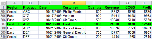
Figure 12.1. Find all Ford records and mark them.
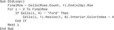
In Chapter 6, you learned to write code like this to color all the Ford records green:
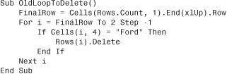
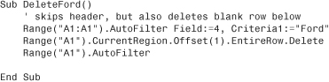
If you needed to delete records, you had to be careful to run the loop from the bottom of the dataset to the top using code like this:
The AutoFilter method enables you to isolate all the Ford records in a single line of code:
Range("A1").AutoFilter Field:=4, Criteria1:="Ford"
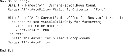
After isolating the matching records, you do not need to use the VisibleCellsOnly setting to format the matching records. Instead, the following line of code will format all the matching records to be green:
Range("A1").CurrentRegion.Interior.ColorIndex = 4
There are two problems with the current two-line macro. First, the program leaves the AutoFilter drop-downs in the dataset. Second, the heading row is also formatted in green.
If you want to turn off the AutoFilter drop-downs and clear the filter, this single line of code will work:
Range("A1").AutoFilter
If you want to leave the AutoFilter drop-downs on but clear the Column D drop-down from showing Ford, you can use this line of code:
ActiveSheet.ShowAllData
The second problem is a bit more difficult. After you apply the filter, select Range("A1"). CurrentRegion includes the headers automatically in the selection. Any formatting is also applied to the header row.
If you did not care about the first blank row below the data, you could simply add an OFFSET(1) to move the current region down to start in A2. This would be fine if your goal were to delete all the Ford records:
Note
The OFFSET property usually requires the number of rows and the number of columns. Using .OFFSET(-2, 5) moves two rows up and five columns right. If you do not want to adjust by any columns, you can leave off the column parameter. .OFFSET(1) means one row down and zero columns over.
The preceding code works because you do not mind if the first blank row below the data is deleted. However, if you are applying a green format to those rows, the code will apply the green format to the blank row below the dataset, which would not look right.
If you will be doing some formatting, you can determine the height of the dataset and use .Resize to reduce the height of the current region while you use OFFSET:
Using New AutoFilter Techniques
Excel 2007 introduced the possibility of selecting multiple items from a filter, filtering by color, filtering by icon, filtering by top 10, and filtering to virtual date filters. Excel 2010 introduces the new search box in the filter drop-down. All these new filters have VBA equivalents, although some of them are implemented in VBA using legacy filtering methods.
Selecting Multiple Items
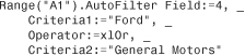
Legacy versions of Excel allowed you to select two values, joined by AND or OR. In this case, you would specify xlAND or xlOR as the operator:
As the AutoFilter command became more flexible, Microsoft continued to use the same three parameters, even if they didn’t quite make sense. For example, Excel lets you filter a field by asking for the top five items or the bottom 8 percent of records. To use this type of filter, specify either "5" or "8" as the Criteria1 argument, and then specify xlTop10Items, xlTop10Percent, xlBottom10Items, xlBottom10Percent as the operator. The following code produces the top 12 revenue records:
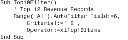
There are a lot of numbers (5, 12, 10) in the code for this AutoFilter. Field 5 indicates that you are looking at the fifth column. xlTop10Items is the name of the filter, but the filter is not limited to 10 items. The criteria of 12 indicates the number of items that you want the filter to return.
Excel 2010 offers several new filter options. Excel continues to force these filter options to fit in the old object model where the filter command must fit in an operator and up to two criteria fields.
If you want to choose three or more items, change the operator to the newly introduced Operator:=xlFilterValues and specify the list of items as an array in the Criteria1 argument:
![]()
Selecting Using the Search Box
Excel 2010 introduces the new Search box in the AutoFilter drop-down. After typing something in the Search box, you can use the Select All Search Results item in the Filter drop-down, as shown in Figure 12.2.
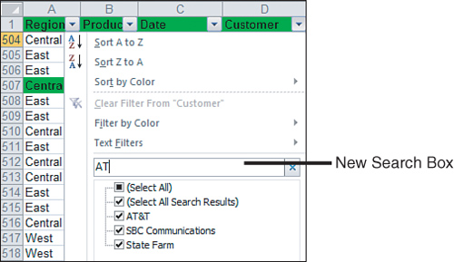
Figure 12.2. Find all records containing “AT.”.
The macro recorder does a poor job of recording the Search box. The macro recorder hard-codes a list of customers who matched the search at the time you ran the macro.
Think about the Search box. It is really a shortcut way of selecting Text Filters, Contains. In addition, the Contains filter is actually a shortcut way of specifying the search string surrounded by asterisks. Therefore, to filter to all the records that contain “AT,” use this:
Range("A1").AutoFilter, Field:=4, Criteria1:="*at*"
Filtering by Color
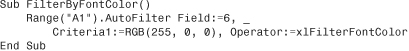
To find records that have a particular font color, use an operator of xlFilterFontColor and specify a particular RGB value as the criteria. This code finds all cells with a red font in Column F:
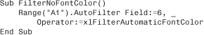
To find records that have no particular font color, use an operator of xlFilterAutomaticFillColor and do not specify any criteria.
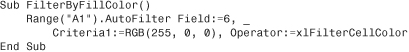
To find records that have a particular fill color, use an operator of xlFilterCellColor and specify a particular RGB value as the criteria. This code finds all red cells in Column F:
To find records that have no fill color, use an operator of xlFilterNoFill and do not specify any criteria.
Filtering by Icon
If you are expecting the dataset to have an icon set applied, you can filter to show only records with one particular icon by using the xlFilterIcon operator.
For the criteria, you have to know which icon set has been applied and which icon within the set. The icon sets are identified using the names shown in Column A of Figure 12.3. The items range from 1 through 5. The following code filters the Revenue column to show the rows containing an upward-pointing arrow in the 5 Arrows Gray icon set:
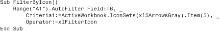
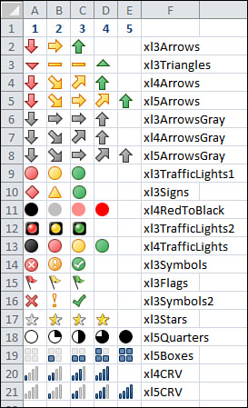
Figure 12.3. To search for a particular icon, you need to know the icon set from Column A and the item number from Row 1.
To find records that have no conditional formatting icon, use an operator of xlFilterNoIcon and do not specify any criteria.
Selecting a Dynamic Date Range Using AutoFilters
Perhaps the most powerful feature in Excel 2010 filters are the dynamic filters. These filters enable you to choose records that are above average or with a date field to select virtual periods, such as Next Week or Last Year.
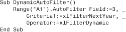
To use a dynamic filter, specify xlFilterDynamic as the operator and then use one of 34 values as Criteria1. The following code finds all dates that are in next year:
The following lists all the dynamic filter criteria options. Specify these values as Criteria1 in the AutoFilter method:
• Criteria for values—Use xlFilterAboveAverage or xlFilterBelowAverage to find all the rows that are above or below average. Note that in Lake Wobegon, using xlFilterBelowAverage will likely return no records.
• Criteria for future periods—Use xlFilterTomorrow, xlFilterNextWeek, xlFilterNextMonth, xlFilterNextQuarter, or xlFilterNextYear to find rows that fall in a certain future period. Note that next week starts on Sunday and ends on Saturday.
• Criteria for current periods—Use xlFilterToday, xlFilterThisWeek, xlFilterThisMonth, xlFilterThisQuarter, or xlFilterThisYear to find rows that fall within the current period. Excel will use the system clock to find the current day.
• Criteria for past periods—Use xlFilterYesterday, xlFilterLastWeek, xlFilterLastMonth, xlFilterLastQuarter, xlFilterLastYear, or xlFilterYearToDate to find rows that fell within a previous period.
• Criteria for specific quarters—Use xlFilterDatesInPeriodQuarter1, xlFilterDatesInPeriodQuarter2, xlFilterDatesInPeriodQuarter3, or xlFilterDatesInPeriodQuarter4 to filter to rows that fall within a specific quarter. Note that these filters do not differentiate based on a year. If you ask for quarter 1, you might get records from this January, last February, and next March.
• Criteria for specific months—Use xlFilterDatesInPeriodJanuary through xlFilterDatesInPeriodDecember to filter to records that fall during a certain month. Like the quarters, the filter does not filter to any particular year.
Unfortunately, you cannot combine criteria. You might think that you can specify xlFilterDatesInPeriodJanuary as Criteria1 and xlFilterDatesNextYear as Criteria2. Even though this is a brilliant thought, Microsoft does not support this syntax (yet).
Selecting Visible Cells Only
Once you apply a filter, most commands only operate on the visible rows in the selection. If you need to delete the records, format the records, apply a conditional format to the records, you can simply refer to the .CurrentRegion of the first heading cell and perform the command.
However, if you have a dataset where the rows have been hidden using the Hide Rows command, any formatting applied to the .CurrentRegion will apply to the hidden rows, too. In these cases, you should use the Visible Cells Only option of the Go To Special dialog, as shown in Figure 12.4.
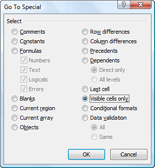
Figure 12.4. If rows have been manually hidden, use Visible Cells Only of the Go To Special dialog.
To use Visible Cells Only in code, use the SpecialCells property:
Range("A1").CurrentRegion.SpecialCells(xlCellTypeVisible)
Case Study: Go To Special Instead of Looping
The Go To Special dialog also plays a role in the following case study:
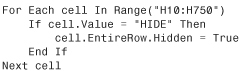
At the 2009 Data Analyst Boot Camp, one of the attendees had a macro that was taking a long time to run. The workbook had a number of selection controls. A complex IF function in cells H10:H750 was choosing which records should be included in a report. While that IF statement had many nested conditions, the formula was inserting either KEEP or HIDE in each cell:
=IF(True,"KEEP","HIDE")
The following section of code was hiding individual rows:
The macro was taking several minutes to run. SUBTOTAL formulas that excluded hidden rows were recalculating after each pass through the loop. The first attempts to speed up the macro involved turning off screen updating and calculation:
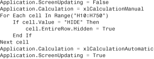
For some reason, it was still taking too long to loop through all the records. We tried using AutoFilter to isolate the HIDE records, then hiding those rows, but you lose the manual row hiding after turning off the AutoFilter.
The solution was to make use of the Special Cells dialog’s ability to limit the selection to text results of formulas. First, the formula in Column H was changed to return either HIDE or a number:
=IF(True,"KEEP",1)
Then, the following single line of code was able to hide the rows that evaluated to a text value in Column H:
![]()
Because all the rows were hidden in a single command, that section of the macro ran in seconds rather than minutes.
![]() To see a demo of this case study, search for Excel VBA 12 at YouTube.
To see a demo of this case study, search for Excel VBA 12 at YouTube.
Advanced Filter Is Easier in VBA Than in Excel
Using the arcane Advanced Filter command is so difficult in the Excel user interface that it is pretty rare to find someone who enjoys using it regularly.
However, in VBA, advanced filters are a joy to use. With a single line of code, you can rapidly extract a subset of records from a database or quickly get a unique list of values in any column. This is critical when you want to run reports for a specific region or customer. Two advanced filters are used most often in the same procedure—one to get a unique list of customers and a second to filter to each individual customer, as shown in Figure 12.5. The rest of this chapter builds toward such a routine.
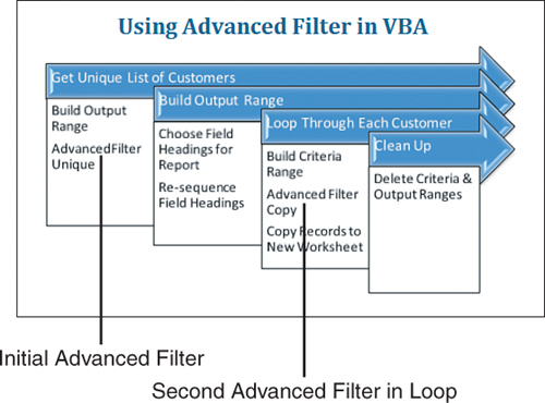
Figure 12.5. A typical macro uses two advanced filters.
Using the Excel Interface to Build an Advanced Filter
Because not many people use the Advanced Filter feature, this section walks you through examples using the user interface to build an advanced filter and then shows you the analogous code. You will be amazed at how complex the user interface seems and yet how easy it is to program a powerful advanced filter to extract records.
One reason why Advanced Filter is hard to use is that you can use the filter in several different ways. You must make three basic choices in the Advanced Filter dialog box. Because each choice has two options, there are eight (2 × 2 × 2) possible combinations of these choices. The three choices are shown in Figure 12.6 and described here:
• Action—You can select Filter the List, In-Place, or Copy to Another Location. If you choose to filter the records in place, the nonmatching rows are hidden. Choosing to copy to a new location copies the records that match the filter to a new range.
• Criteria—You can filter with or without criteria. Filtering with criteria is appropriate for getting a subset of rows. Filtering without criteria is still useful when you want a subset of columns or when you are using the Unique Records Only option.
• Unique—You can choose to request Unique Records Only or all matching records. The Unique option makes the Advanced Filter command one of the fastest ways to find a unique list of values in one field. By placing the “Customer” heading in the output range, you will get a unique list of values for that one column.
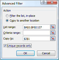
Figure 12.6. The Advanced Filter dialog is complicated to use in the Excel user interface. Luckily, it is much easier in VBA.
Using Advanced Filter to Extract a Unique List of Values
One of the simplest uses of Advanced Filter is to extract a unique list of a single field from a dataset. In this example, you want to get a unique list of customers from a sales report. You know that customer is in Column D of the dataset. You have an unknown number of records starting in cell A2, and Row 1 is the header row. There is nothing located to the right of the dataset.
Extracting a Unique List of Values with the User Interface
To extract a unique list of values, follow these steps:
- With the cursor anywhere in the data range, select Advanced from the Sort & Filter group on the Data tab. The first time that you use the Advanced Filter command on a worksheet, Excel automatically populates the List Range text box with the entire range of your dataset. On subsequent uses of the Advanced Filter command, this dialog box remembers the settings from the prior advanced filter.
- Select the Unique Records Only check box at the bottom of the dialog.
- In the Action section, select Copy to Another Location.
- Type
J1in the Copy To text box.
By default, Excel copies all the columns in the dataset. You can filter just the Customer column by either limiting the List Range to include only Column D or by specifying one or more headings in the Copy To range. Either method has its own drawbacks.
Change the List Range to a Single Column
Edit the List Range to point to the Customer column. In this case, it means changing the default $A$1:$H$1127 to $D$1:$D$1127. The Advanced Filter dialog should appear.
Tip
When you initially edit any range in the dialog box, Excel might be in Point mode. In this mode, pressing a left- or right-arrow key will insert a cell reference in the text box. If you see the word Point in the lower-left corner of your Excel window, press the F2 key to change from Point mode to Edit mode.
The drawback of this method is that Excel remembers the list range on subsequent uses of the Advanced Filter command. If you later want to get a unique list of regions, you will be constantly specifying the list range.
Copy the Customer Heading Before Filtering
With a little forethought before invoking the Advanced Filter command, you can allow Excel to keep the default list range of $A$1:$H$1127. In cell J1, type the Customer heading. In Figure 12.6, you leave the List Range field pointing to Columns A through H. Because the Copy To range of J1 already contains a valid heading from the list range, Excel copies data only from the Customer column. This is the preferred method, particularly if you will be doing multiple advanced filters. Because Excel remembers the prior settings from the last advanced filter, it is more convenient to always filter the entire columns of the list range and limit the columns by setting up headings in the Copy To range.
After you use either of these methods to perform the advanced filter, a concise list of the unique customers appears in Column J (see Figure 12.7).
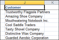
Figure 12.7. The advanced filter extracted a unique list of customers from the dataset and copied it to Column J.
Extracting a Unique List of Values with VBA Code
In VBA, you use the AdvancedFilter method to carry out the Advanced Filter command. Again, you have three choices to make:
• Action—Choose to either filter in place with the parameter Action:=xlFilterInPlace or to copy with Action:=xlFilterCopy. If you want to copy, you also have to specify the parameter CopyToRange:=Range("J1").
• Criteria—To filter with criteria, include the parameter CriteriaRange:=Range("L1:L2"). To filter without criteria, omit this optional parameter.
• Unique—To return only unique records, specify the parameter Unique:=True.
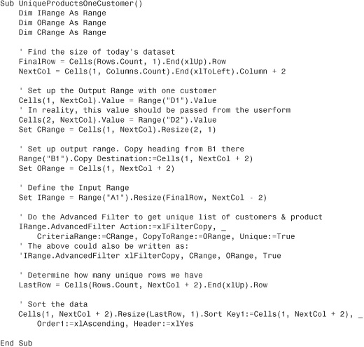
The following code sets up a single column output range two columns to the right of the last-used column in the data range:
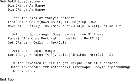
By default, an advanced filter copies all columns. If you just want one particular column, use that column heading as the heading in the output range.
The first bit of code finds the final row and column in the dataset. Although it is not necessary to do so, you can define an object variable for the output range (ORange) and for the input range (IRange).
This code is generic enough that it will not have to be rewritten if new columns are added to the dataset at a later time. Setting up the object variables for the input and output range is done for readability rather than out of necessity. The previous code could be written just as easily like this shortened version:
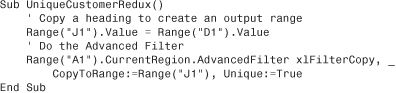
When you run either of the previous blocks of code on the sample dataset, you get a unique list of customers off to the right of the data. In Figure 12.7, you saw the original dataset in Columns A:H and the unique customers in Column J. The key to getting a unique list of customers is copying the header from the Customer field to a blank cell and specifying this cell as the output range.
After you have the unique list of customers, you can sort the list and add a SUMIF formula to get total revenue by customer. The following code gets the unique list of customers, sorts it, and then builds a formula to total revenue by customer. Figure 12.8 shows the results:
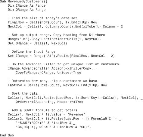
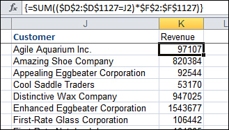
Figure 12.8. This macro produced a summary report by customer from a lengthy dataset. Using AdvancedFilter is the key to powerful macros such as these.
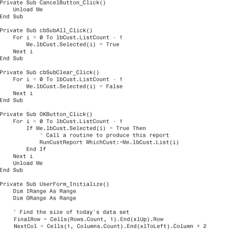
Another use of a unique list of values is to quickly populate a list box or a combo box on a userform. For example, suppose that you have a macro that can run a report for any one specific customer. To allow your clients to choose which customers to report, create a simple userform. Add a list box to the userform and set the list box’s MultiSelect property to 1-fmMultiSelectMulti. In this case, the form is named frmReport. In addition to the list box, there are four command buttons: OK, Cancel, Mark All, Clear All. The code to run the form follows. Note the Userform_Initialize procedure includes an advanced filter to get the unique list of customers from the dataset:

Launch this form with a simple module such as this:
Sub ShowCustForm()
frmReport.Show
End Sub
Your clients are presented with a list of all valid customers from the dataset. Because the list box’s MultiSelect property is set to allow it, they can select any number of customers, as shown in Figure 12.9.
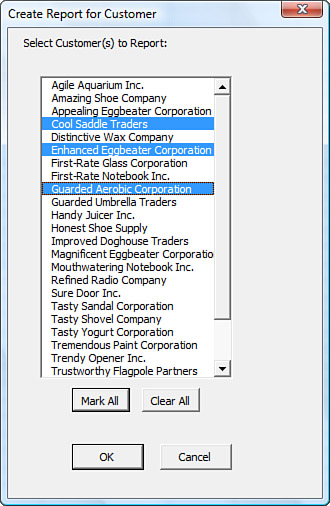
Figure 12.9. Your clients will have a list of customers from which to select. Using an advanced filter on even a 1,000,000-row dataset is much faster than setting up a class to populate the list box.
Getting Unique Combinations of Two or More Fields
To get all unique combinations of two or more fields, build the output range to include the additional fields. This code sample builds a list of unique combinations of two fields, Customer and Product:
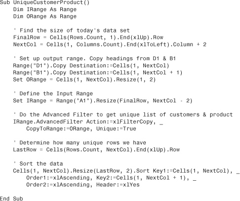
In the result shown in Figure 12.10, you can see that Enhanced Eggbeater buys only one product, and Agile Aquarium buys three products. This might be useful to use as a guide in running reports on either customer by product or product by customer.
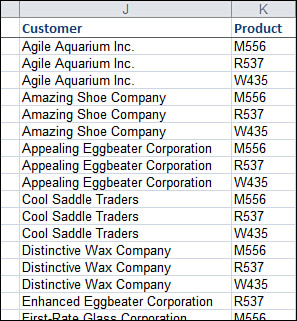
Figure 12.10. By including two columns in the output range on a Unique Values query, we get every combination of Customer and Product.
Using Advanced Filter with Criteria Ranges
As the name implies, Advanced Filter is usually used to filter records—in other words, to get a subset of data. You specify the subset by setting up a criteria range. Even if you are familiar with criteria, be sure to check out using the powerful Boolean formula in criteria ranges later in this chapter, in the section “The Most Complex Criteria: Replacing the List of Values with a Condition Created as the Result of a Formula.”
Set up a criteria range in a blank area of the worksheet. A criteria range always includes two or more rows. The first row of the criteria range contains one or more field header values to match the one(s) in the data range you want to filter. The second row contains a value showing what records to extract. In Figure 12.11, Range J1:J2 is the criteria range, and Range L1 is the output range.
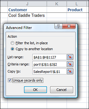
Figure 12.11. To learn a unique list of products purchased by Cool Saddle Traders, set up the criteria range shown in J1:J2.
In the Excel user interface, to extract a unique list of products that were purchased by a particular customer, select Advanced Filter and set up the Advanced Filter dialog, as shown in Figure 12.11. Figure 12.12 shows the results.
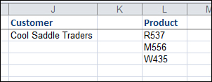
Figure 12.12. The results of the advanced filter that uses a criteria range and asks for a unique list of products. Of course, more complex and interesting criteria can be built.
In VBA, you use the following code to perform an equivalent advanced filter:
Joining Multiple Criteria with a Logical OR
You might want to filter records that match one criteria or another. For example, you can extract customers who purchased either product M556 or product R537. This is called a logical OR criteria.
When your criteria should be joined by a logical OR, place the criteria on subsequent rows of the criteria range. For example, the criteria range shown in J1:J3 of Figure 12.13 tells you which customers order product M556 or product R357.
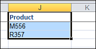
Figure 12.13. Place criteria on successive rows to join them with an OR. This criteria range gets customers who ordered either product M556 or R537.
Joining Two Criteria with a Logical AND
Other times, you will want to filter records that match one criteria and another criteria. For example, you might want to extract records where the product sold was W435 and the region was the West region. This is called a logical AND.
To join two criteria by AND, put both criteria on the same row of the criteria range. For example, the criteria range shown in J1:K2 of Figure 12.14 gets the customers who ordered product W435 in the West region.
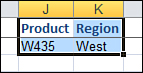
Figure 12.14. Place criteria on the same row to join them with an AND. The criteria range in J1:K2 gets customers from the West region who ordered product W435.
Other Slightly Complex Criteria Ranges
The criteria range shown in Figure 12.15 is based on two different fields that are joined with an OR. The query finds all records from either the West region or records where the product is W435.

Figure 12.15. The criteria range in J1:K3 returns records where either the Region is West or the Product is W435.
Tip
Joining two criteria with OR might be useful where new California legislation will impact shipments made to California or products sourced at the California plant.
The Most Complex Criteria: Replacing the List of Values with a Condition Created as the Result of a Formula
It is possible to have a criteria range with multiple logical AND and logical OR criteria joined together. Although this might work in some situations, in other scenarios it quickly gets out of hand. Fortunately, Excel allows for criteria where the records are selected as the result of a formula to handle this situation.
Case Study: Working with Very Complex Criteria
Your clients so loved the “Create a Customer” report, they hired you to write a new report. In this case, they could select any customer, any product, any region, or any combination of them. You can quickly adapt the frmReport userform to show three list boxes, as shown in Figure 12.16.
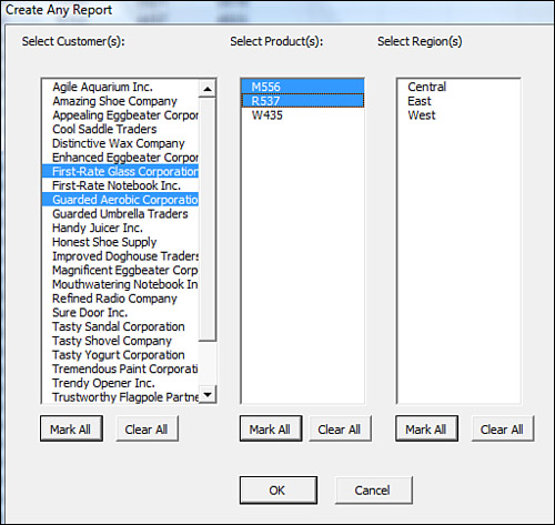
Figure 12.16. This super-flexible form lets clients run any types of reports that they can imagine. It creates some nightmarish criteria ranges, unless you know the way out.
In your first test, imagine that you select two customers and two products. In this case, your program has to build a five-row criteria range, as shown in Figure 12.17. This isn’t too bad.
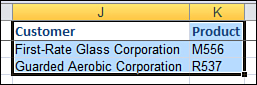
Figure 12.17. This criteria range returns any records where the two selected customers ordered any of the two selected products.
This gets crazy if someone selects 10 products, all regions but the house region, and all customers except the internal customer. Your criteria range would need unique combinations of the selected fields. This could easily be 10 products times 9 regions times 499 customers, or more than 44,000 rows of criteria range. You can quickly end up with a criteria range that spans thousands of rows and three columns. I was once foolish enough to actually try running an advanced filter with such a criteria range. It would still be trying to compute if I hadn’t rebooted the computer.
The solution for this report is to replace the lists of values with a formula-based condition.
Setting Up a Condition as the Result of a Formula
Amazingly, there is an incredibly obscure version of Advanced Filter criteria that can replace the 44,000-row criteria range in the previous case study. In the alternative form of criteria range, the top row is left blank. There is no heading above the criteria. The criteria set up in Row 2 are a formula that results in True or False. If the formula contains any relative references to Row 2 of the data range, Excel compares that formula to every row of the data range, one by one.
For example, if you want all records where the Gross Profit Percentage is below 53 percent, the formula built in J2 will reference the Profit in H2 and the Revenue in F2. To do this, leave J1 blank to tell Excel that you are using a computed criterion. Cell J2 contains the formula =(H2/F2)<0.53. The criteria range for the advanced filter would be specified as J1:J2.
As Excel performs the advanced filter, it logically copies the formula and applies it to all rows in the database. Anywhere that the formula evaluates to True, the record is included in the output range.
This is incredibly powerful and runs remarkably fast. You can combine multiple formulas in adjacent columns or rows to join the formula criteria with AND or OR, just as you do with regular criteria.
Note
Row 1 of the criteria range doesn’t have to be blank, but it cannot contain any words that are headings in the data range. You could perhaps use that row to explain that someone should look to this page in this book for an explanation of these computed criteria.
Case Study: Using Formula-Based Conditions in the Excel User Interface
You can use formula-based conditions to solve the report introduced in the previous case study. Figure 12.18 shows the flow of setting up a formula-based criteria.
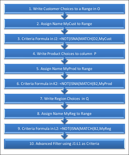
Figure 12.18. Data in O:Q is used in formulas in J2:L2.
To illustrate, off to the right of the criteria range set up a column of cells with the list of selected customers. Assign a name to the range, such as MyCust. In cell J2 of the criteria range, enter a formula such as =Not(ISNA(Match(D2,MyCust,0))).
To the right of the MyCust range, set up a range with a list of selected products. Assign this range the name of MyProd. In the K2 of the criteria range, add a formula to check products, =NOT(ISNA(Match(B2,MyProd,0))).
To the right of the MyProd range, set up a range with a list of selected regions. Assign this range the name of MyRegion. In L2 of the criteria range, add a formula to check for selected regions, =NOT(ISNA(Match(A2,MyRegion,0))).
Now, with a criteria range of J1:L2, you can effectively retrieve the records matching any combination of selections from the userform.
Using Formula-Based Conditions with VBA
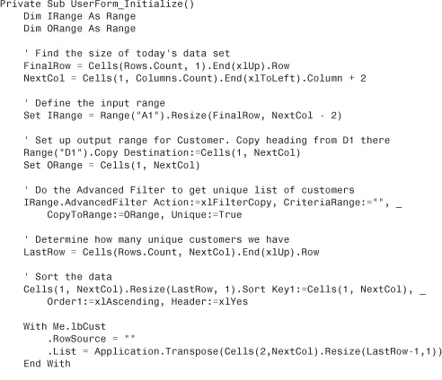
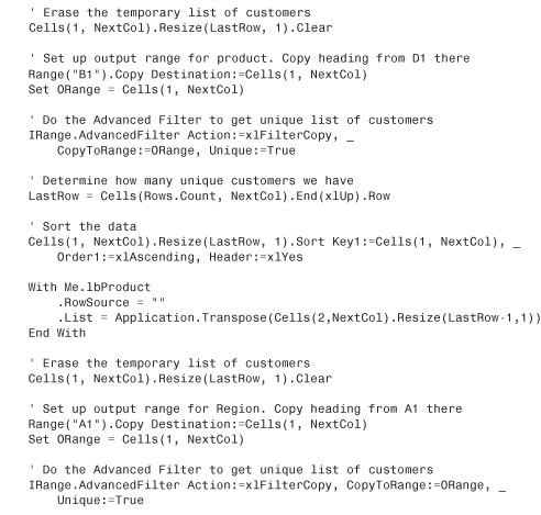
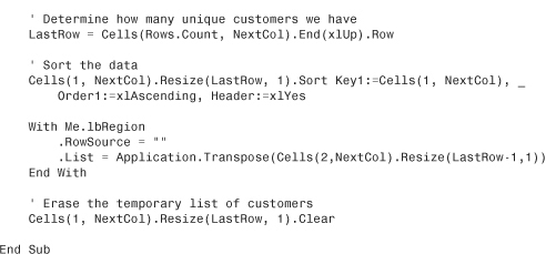
The following is the code for this userform. Note the logic in OKButton_Click that builds the formula. Figure 12.19 shows the Excel sheet just before the advanced filter is run.

Figure 12.19. The worksheet just before the macro runs the advanced filter.
The following code initializes the user form. Three advanced filters find the unique list of customers, products, and regions:
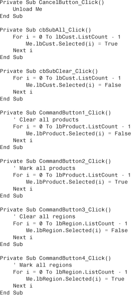
These tiny procedures run when someone clicks Mark All or Clear All:
The following code is attached to the OK button. This code builds three ranges in O, P, and Q that list the selected customers, products, and regions. The actual criteria range is comprised of three blank cells in J1:L1 and then three formulas in J2:L2.
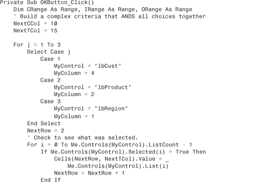
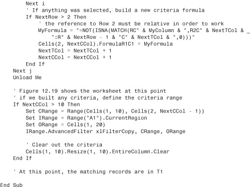
Figure 12.19 shows the worksheet just before the AdvancedFilter method is called. The user has selected customers, products, and regions. The macro has built temporary tables in Columns O, P, Q to show which values the user selected. The criteria range is J1:L2. That criteria formula in J2 looks to see whether the value in $D2 is in the list of selected customers in O. The formulas in K2 and L2 compare $B2 to Column P and $A2 to Column Q.
Caution
Excel VBA Help says that if you do not specify a criteria range, no criteria is used. This is not true in Excel 2010. When working with Excel 2010, if no criteria range is specified, the advanced filter inherits the criteria range from the prior advanced filter. You should include CriteriaRange:="" to clear the prior value.
Using Formula-Based Conditions to Return Above-Average Records
The formula-based conditions formula criteria are cool but are a rarely used feature in a rarely used function. Some interesting business applications use this technique. For example, this criteria formula would find all the above-average rows in the dataset:
=$A2>Average($A$2:$A$60000)
Using Filter in Place in Advanced Filter
It is possible to filter a large dataset in place. In this case, you do not need an output range. You would normally specify criteria range—otherwise you return 100 percent of the records and there is no need to do the advanced filter!
In the user interface of Excel, running a Filter in Place makes sense: You can easily peruse the filtered list looking for something in particular.
Running a Filter in Place in VBA is a little less convenient. The only good way to programmatically peruse through the filtered records is to use the xlCellTypeVisible option of the SpecialCells method. In the Excel user interface, the equivalent action is to select Find & Select, Go to Special from the Home tab. In the Go to Special dialog, select Visible Cells Only, as shown in Figure 12.20.
Figure 12.20. The Filter in Place option hides rows that do not match the selected criteria. However, the only way to programmatically see the matching records is to do the equivalent of selecting Visible Cells Only from the Go To Special dialog box.
To run a Filter in Place, use the constant XLFilterInPlace as the Action parameter in the AdvancedFilter command and remove the CopyToRange from the command:
![]()
Then, the programmatic equivalent to loop through Visible Cells Only is this code:
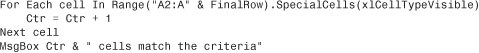
If you know that there would be no blanks in the visible cells, you could eliminate the loop with
Ctr = Application.Counta(Range("A2:A" & FinalRow).SpecialCells(xlCellTypeVisible))
Catching No Records When Using Filter in Place
Just as when using Copy, you have to watch out for the possibility of having no records match the criteria. However, in this case it is more difficult to realize that nothing is returned. You generally find out when the .SpecialCells method returns a Runtime Error 1004—no cells were found.
To catch this condition, you have to set up an error trap to anticipate the 1004 error with the SpecialCells method.
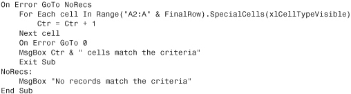
This error trap works because it specifically excludes the header row from the SpecialCells range. The header row is always visible after an advanced filter. Including it in the range would prevent the 1004 error from being raised.
Showing All Records After Filter in Place
After doing a Filter in Place, you can get all records to show again by using the ShowAllData method:
ActiveSheet.ShowAllData
The Real Workhorse: xlFilterCopy with All Records Rather Than Unique Records Only
The examples at the beginning of this chapter talked about using xlFilterCopy to get a unique list of values in a field. You used unique lists of customer, region, and product to populate the list boxes in your report-specific userforms.
However, a more common scenario is to use an advanced filter to return all records that match the criteria. After the client selects which customer to report, an advanced filter can extract all records for that customer.
In all the examples in the following sections, you want to keep the Unique Records Only check box cleared. You do this in VBA by specifying Unique:=False as a parameter to the AdvancedFilter method.
This is not difficult to do, and you have some powerful options. If you need only a subset of fields for a report, copy only those field headings to the output range. If you want to resequence the fields to appear exactly as you need them in the report, you can do this by changing the sequence of the headings in the output range.
The next sections walk you through three quick examples to show the options available.
Copying All Columns
To copy all columns, specify a single blank cell as the output range. You will get all columns for those records that match the criteria, as shown in Figure 12.21:
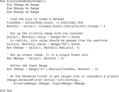
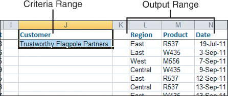
Figure 12.21. When using xlFilterCopy with a blank output range, you get all columns in the same order as they appear in the original list range.
Copying a Subset of Columns and Reordering
If you are doing the advanced filter to send records to a report, it is likely that you might only need a subset of columns and you might need them in a different sequence.
This example finishes the frmReport example that was presented earlier in this chapter. As you recall, frmReport allows the client to select a customer. The OK button then calls the RunCustReport routine, passing a parameter to identify for which customer to prepare a report.
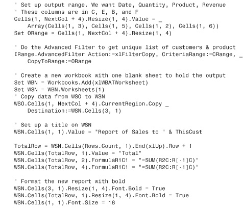
Imagine this is a report being sent to the customer. The customer really does not care about the surrounding region, and you do not want to reveal your cost of goods sold or profit. Assuming that you will put the customer’s name in the title of the report, the fields that you need to produce the report are Date, Quantity, Product, Revenue.
The following code copies those headings to the output range. The advanced filter produces data, as shown in Figure 12.22. The program then goes on to copy the matching records to a new workbook. A title and total row is added, and the report is saved with the customer’s name. Figure 12.23 shows the final report.
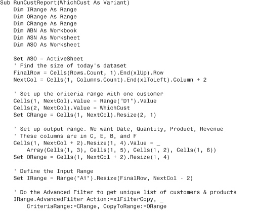
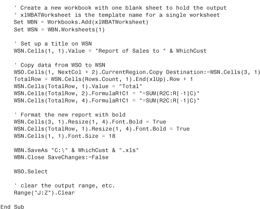
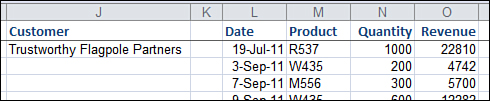
Figure 12.22. Immediately after the advanced filter, you have just the columns and records needed for the report.
Figure 12.23. After copying the filtered data to a new sheet and applying some formatting, you have a good-looking report to send to each customer.
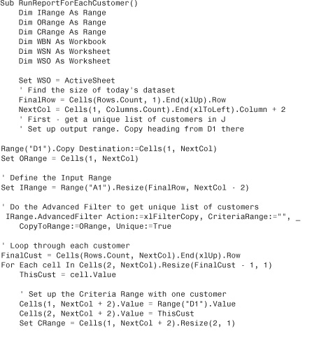
Case Study: Utilizing Two Kinds of Advanced Filters to Create a Report for Each Customer
The final advanced filter example for this chapter uses several advanced filter techniques. Let’s say that after importing invoice records, you want to send a purchase summary to each customer. The process would be as follows:
- Run an advanced filter requesting unique values to get a list of customers in J. This
AdvancedFilterspecifies theUnique:=Trueparameter and uses aCopyToRangethat includes a single heading for Customer: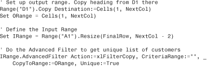
- For each customer in the list of unique customers in Column J, perform steps 3 through 7. Find the number of customers in the output range from step 1. Then, use a
For Each Cellloop to loop through the customers: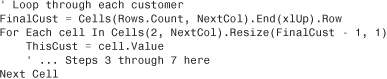
- Build a criteria range in L1:L2 to be used in a new advanced filter. The criteria range would include a heading of Customer in L1 and the customer name from this iteration of the loop in cell L2:
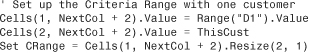
- Do an advanced filter to copy matching records for this customer to Column N. This
Advanced Filterstatement specifies theUnique:=Falseparameter. Because you want only the columns for Date, Quantity, Product, and Revenue, theCopyToRangespecifies a four-column range with those headings copied in the proper order: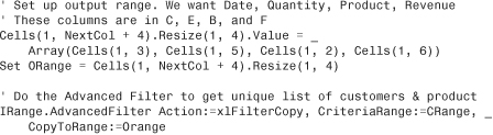
- Copy the customer records to a report sheet in a new workbook. The VBA code uses the
Workbooks.Addmethod to create a new blank workbook. The extracted records from step 4 are copied to Cell A3 of the new workbook: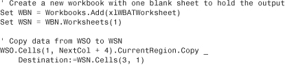
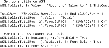
- Format the report with a title and totals. In VBA, add a title that reflects the customer’s name in cell A1. Make the headings bold and add a total below the final row:
- Use
SaveAsto save the workbook based on customer name. After the workbook is saved, close the new workbook. Return to the original workbook and clear the output range to prepare for the next pass through the loop: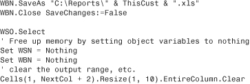
The complete code is as follows:
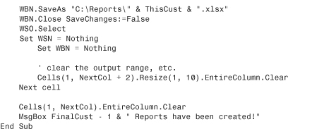
This is a remarkable 45 lines of code. Incorporating a couple of advanced filters and not much else, you have managed to produce a tool that created 27 reports in less than 1 minute. Even an Excel power user would normally take 2 to 3 minutes per report to create these manually. In less than 60 seconds, this code will save someone a few hours every time these reports need to be created. Imagine the real scenario where there are hundreds of customers. Undoubtedly, there are people in every city who are manually creating these reports in Excel because they simply don’t realize the power of Excel VBA.
Using Filter in Place with Unique Records Only
It is possible to use Filter in Place and Unique Records Only. Only columns that should be evaluated for unique combinations of values should be specified as the input range.
In Figure 12.24, the dataset has a common problem: Each account number appears with many different spellings of the customer name. You would like a unique list of customer numbers. For each unique customer number, you would like to include any of the various spellings for that customer.
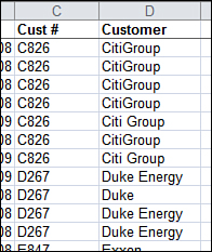
Figure 12.24. Each account number has various variations of customer name.
To solve this problem, you can specify Column C as the input range, filter in place, and ask for unique records using this code:
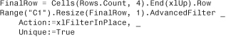
Figure 12.25 shows the result: Each account number appears just once.
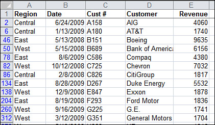
Figure 12.25. Because Column C was the input range, you only see one line per customer number.
Column D contains the first instance of each customer name. To copy those results to another place, use this code.
![]()
Figure 12.26 shows a unique list of customer numbers with the first customer name found for each customer number. This is significantly different than using Remove Duplicates on Customer Number and Customer. That command would show each variant of spelling of the customer name as a new row.
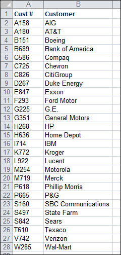
Figure 12.26. A unique list of customer numbers, along with one of the spellings of the customer name.
Excel in Practice: Turning Off a Few Drop-Downs in the AutoFilter
One cool feature is available only in Excel VBA. When you AutoFilter a list in the Excel user interface, every column in the dataset gets a field drop-down in the heading row. Sometimes you have a field that does not make a lot of sense to AutoFilter. For example, in your current dataset, you might want to provide AutoFilter drop-downs for Region, Product, Customer, but not the numeric or date fields. After setting up the AutoFilter, you need one line of code to turn off each drop-down that you do not want to appear. The following code turns off the drop-downs for Columns C, E, F, G, and H:
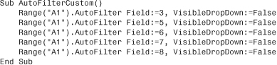
Using this tool is a fairly rare treat. Most of the time, Excel VBA lets you to do things that are possible in the user interface—although it lets us do them very rapidly. The VisibleDropDown parameter actually enables you to do something in VBA that is generally not available in the Excel user interface. Your knowledgeable clients will be scratching their heads trying to figure out how you set up the cool auto filter with only a few filterable columns (see Figure 12.27).
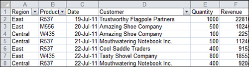
Figure 12.27. Using VBA, you can set up an auto filter where only certain columns have the AutoFilter drop-down.
To clear the filter from the customer column, you use this code:

Next Steps
Using techniques from this chapter, you have many reporting techniques available to you by using the arcane Advanced Filter tool. Chapter 13, “Using VBA to Create Pivot Tables,” introduces the most powerful feature in Excel: the pivot table. The combination of advanced filters and pivot tables creates reporting tools that enable amazing applications.