CHAPTER 7

The Behavior of a Coin

Making Predictions with Probability

I’m gamblin’,
Gamble all over town. . . .
Yea, where I meet with a deck of cards,
Boy you know I lay my money down. —Lightnin’ Hopkins, “The Roving Gambler”

My great books course professor relayed an anecdote about Flaubert. The professor himself wore a stained, tan trench coat during the hour and, with his difficulty of getting Bs out without stuttering them, told our class that Flaubert, the author of Madame B-B-B-Bovary, had a catalogue of writing exercises that he shared with his friend Maxime du Camp.¹ The two would have lunch in small Paris restaurants and often would try to match the coats on the coat rack with the clientele of the place, just by observing features, mannerisms, and expressions. I have no idea how true or apocryphal the story is, but anyone reading passages of Madame Bovary would well believe it. See how carefully Flaubert describes Charles Bovary, a young boy about to enter lycée.

The Newcomer, who was hanging back in the corner so that the door half hid him from view, was a country lad of about fifteen, taller than any of us. He had his hair cut in bangs like a cantor in a village church, and he had a gentle timid look. He wasn’t broad in the shoulders, but his green jacket with its black buttons seemed tight under the arms; and through the vents of his cuffs we could see red wrists that were clearly unaccustomed to being covered. His yellowish breeches were hiked up by his suspenders, and from them emerged a pair of blue-stockinged legs. He wore heavy shoes, hobnailed and badly shined.²

In this description, Flaubert is setting us up with a heuristic representation of a boy who will very quickly become a country doctor in the novel. In fact, we are not surprised to learn that this country doctor is merely an officier de santé, a person schooled in medicine not holding a medical degree.³

You are wondering why I bring this story up in a book on gambling. Flaubert’s novels are filled with heuristic representations that make us believe we are right when we match the coat with the person. It is what all good novelists do. Reading novels is often an exercise in making heuristic judgments. In real life we make such matches all the time. They are the routine judgments we make, and they come from beliefs driven by stereotyped circumstances. Without conscious awareness, we make probabilistic judgments about people, events, and outcomes based on a very limited number of vague and dubious assumptions coming from our internal hypotheses. Suppose you read that a fellow by the name of Steve is very shy and withdrawn, invariably helpful, but that he has little interest in people or in the world of reality. He is submissive with a need for order and structure.⁴ Now order Steve’s most likely occupations from the following list: farmer, salesman, airline pilot, librarian, and physician. We have a strong sense that if the list includes Steve’s true occupation, then he is most likely to be a librarian and least likely to be an airline pilot. Why shouldn’t Steve be an airline pilot? Or, more to the point, why shouldn’t the job of pilot be the most likely—consider his need for order and structure, as well as his passion for detail.

Steve seems to have been represented as the stereotypic librarian, not as the stereotypic airline pilot. The problem here is that two measures are confused—likelihood and stereotype. Research shows that most people tend to have that confusion.⁵ But there is something else going on here. Shouldn’t it be more likely that Steve is a farmer? After all, there are many more farmers than librarians. If we simply evaluate Steve as a man obeying some random frequency distribution, he would more likely be a farmer. However, under normal heuristic tendencies the probabilistic frequency of farmers in the overall population does not trump considerations of stereotypic similarities, and so we think that he is more likely to be a librarian. In 1973, Amos Tversky and Daniel Kahneman conducted research to study how subjects consider probabilistic as opposed to stereotypic judgments. There were two groups. In one, the subjects were given character descriptions and told that they were from a pool of 70 engineers and 30 lawyers. The other was given the same character descriptions and told that they were from a pool of 30 engineers and 70 lawyers. The subjects in the first group would have a better (probabilistic) chance of being right by simply guessing the character to be an engineer. Similarly, the subjects of the second group might have guessed the character to be a lawyer. But the result of the study determined that people tend to ignore the odds and bank on the descriptive representation of character with no consideration of majority.

More surprisingly, majority representation is ignored, even when the description is uninformative. The following description contains no information about the character’s occupation: “Dick is a thirty-year-old man. He is married with no children. A man of high ability and high motivation, he promises to be quite successful in his field. He is well liked by his colleagues.”

We should expect that subjects would consider the odds of 7 to 3 in favor of being an engineer if the pool contains 70 engineers and 30 lawyers. But that’s not what happens. Subjects simply gave Dick even odds of being an engineer or lawyer.⁶

This discounting of relative pool sizes reflects an insensitivity to sample size. Consider the answers to the following question by 95 undergraduates after they were told that 50 percent of all babies are boys and that in a certain town there is a large hospital where about 45 babies are born each day and a small hospital where about 15 babies are born each day. The students were told that for one year each hospital recorded the number of days in which more than 60 percent of the babies born were boys and asked the following question:

Which hospital do you think recorded more such days?

• The larger hospital (21)

• The smaller hospital (21)

• About the same (that is, within 5 percent of each other) (53).⁷

The surprise here is that students are not paying close attention to the probabilistic logic that suggests the smaller hospital is more likely to report more days when the male proportion exceeds 60 percent. This is simply because the larger hospital has a larger sample and is therefore less likely to deviate from the norm.

Such studies point to misconceptions of chance. People tend to misinterpret the law of large numbers as saying that a long sequence of reds in the spin of a roulette wheel should favor black’s turn. You might think that the sequence R-B-R-B-B-R is more likely than the sequence R-R-R-B-B-B, simply because this latter sequence does not appear to suggest true randomness. According to Tversky and Kahneman, people expect that the important characteristics will be represented in each of its specific local parts.⁸ Yet, that’s not how chance works! Representations of smaller samples deviate from the global expectation. We expect local and regular self-corrections, whereas what we find is simply a gradual dilution of local events as the number of trials increase.

One further point to be raised is the notion of anchoring. We all have a tendency to anchor our opinions to some immediate bias. Consider another experiment conducted by Tversky and Kahneman in which subjects were asked to guess the percentage of African countries listed as members of the United Nations (in 1974). A wheel marked with numbers from 0 to 100 was spun. The wheel would come to rest at a number, say X. The subjects were asked to first indicate whether X was higher or lower than the answer to the question. Following that, the subjects were asked to estimate the value of the quantity by moving upward or downward from that number. The bizarre outcome was that, for the group that saw the wheel land on 10, the median estimate of the percentage of African countries that were members of the United Nations was 25, and for the group that saw the wheel land on 65, the median estimate was 45. Now what does a wheel of fortune have to do with the number of countries belonging to the United Nations?

It seems that humans have definite cognitive biases that are affected by how questions are framed. We might expect that these biases influence a layman’s decisions; surprisingly, they also influence the intuitive judgments of the experienced researcher as well.⁹

Our more rational judgment embraces underlying probabilities and hence a more rational understanding that perhaps there are some mathematical models that could be used to enhance our judgment of the stochastic world. When we consider flipping a fair coin we all know that the probability of it coming up heads is 1/2. The law of large numbers tells us that the ratio of the number of heads to the number of tails approaches 1 as the number of flips grows larger. Heuristic judgment muddles the meaning into a belief that somehow a long string of tails will be made up by a balancing string of heads. The general public continues to confuse the proper meaning of the law of large numbers with the feeling—and erroneous belief—that if a face has not come up for a very long time, the chances of its appearance increase with every turn. And yet that same public knows that theoretically, every time a coin is flipped and every time a roulette wheel is spun the odds against each outcome are precisely the same—the coin is just as likely to land on heads as tails and the roulette ball is just as likely to fall into any one stall as into any other. It’s just that people tend to muddle the difference between outcomes and frequencies.

Toyota Prius drivers have played with this law. The Prius displays the average miles per gallon and that figure can be reset. When starting out on a journey of, say, 500 miles, the displayed number fluctuates depending on driving conditions. In the first 10 miles the display may read, say, 52.3 miles per gallon. At 20 miles it may read 46.4 miles per gallon. New Prius owners tend to hypermile; that is, they tend to drive in a manner that maximizes the average miles per gallon. Generally this means managing the gas pedal with an awareness of its effect on the miles per gallon on the display screen. They quickly notice that the fluctuation is wild for the first ten, twenty, thirty miles, and that that wildness tends to dampen into a stable range that narrows more and more toward some limiting number. By 200 miles, the display may read 51.2 miles per gallon. At that point even the most skillful hypermiling will not change the display by more than a few tenths. This is because the car’s miles per gallon history is on the side of the accumulated average. If the average of ten numbers is 46.4 and we throw in five more numbers, say, 59, 56, 62, 58, and 57, the average of the fifteen numbers is 50.4, a difference of 5. However, if the average of one hundred numbers is 46.4 and we throw in those same five numbers, the average is just 47, a difference of 0.6.

Figure 7.1 represents the cumulative outcome of 10,000 repeated coin flips (+1 for each head and –1 for each tail).¹⁰ The horizontal line represents 0. So, for example, after approximately 2,500 flips, the outcome is approximately –20. In this particular run, tails is in the lead almost 97 percent of the time. It is a horse race between two horses of equal odds. Normal intuitive judgment favors the opinion that the graph should bounce over and below the zero line far more often than is pictured. However, true mathematical theory tells us that it is far more likely for the graph to favor one side over the other for relatively long periods of time.¹¹ The reason is that once the cumulative outcome strays far from 0 in the negative direction, it needs long strings of heads to get it back to positive territory.¹²

The cumulative record of coin flips may be modeled through a Galton board. Sir Francis Galton, the nineteenth-century English geneticist, constructed a board filled with pegs arranged with a funnel at the top and chambers at the bottom, as in figure 7.2. Galton’s point was to demonstrate that physical events ride on the tailwinds of chance. The ball falls to the first pin and must decide whether to fall left or right. Being unstable in its decision, it does something equivalent to flipping an unbiased coin: heads go left, tails go right. Whichever way it goes, it falls to the next pin and must decide all over again. What does this really mean? Imagine the perfect Galton board as one in which the balls always fall directly on the absolute tops of pegs. What makes the ball fall to the right or left? We said that it was like a coin flip. But that flip may be determined by a history of dependent events initiated by a minuscule perturbation, such as a butterfly flapping its wings over the Pacific or a cow farting in an Idaho cornfield. Before each coin flip, the outcome of the previous flip is history; the coin no longer remembers the outcome and therefore will behave as if it is a new coin. However, the cumulative outcome does take into account the history of all previous coin flips.

FIGURE 7.1. Cumulative outcome of 10,000 repeated coin flips.
SOURCE: “Leads in Coin Tossing,” http://demonstrations.wolfram.com/LeadsInCoinTossing/. With permission under the guidelines of http://creativecommons.org/licenses/by-nc-sa/3.0/.

FIGURE 7.2. A Galton board.

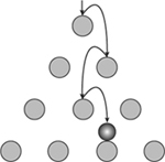
FIGURE 7.3. A bounce off the top peg of a Galton board.

A bounce off the top peg goes left because . . . well, we don’t exactly know why—just because something remotely connected happened, an undetectable air current or vibration. But it represents one of the many unaccounted measurements that imperceptibly affect the outcome. It rolls off the peg to fall directly over the next peg down and, this time, goes right because . . . who knows?

The 50-50 chance of going left or right causes the build-up of the bell-shaped curve marked by the highest balls in figure 7.2. Counting the number of ways the balls can fall proves this. Suppose that a ball is dropped and we mark its descent by the letters L and R to indicate bouncing to the left or right. We would then have the following possible outcomes:

 

LLLL

LLLR, LLRL, LRLL, RLLL

LLRR, LRLR, LRRL, RLLR, RLRL, RRLL

LRRR, RLRR, RRLR, RRRL

RRRR

There are more combinations of mixed letters than non-mixed and since there is an equal chance for the ball to go left or right there is a tendency for it to end in the center slot of the Galton board.

Every event in nature has to account for a vast number of indeterminate possibilities. The toss of a die may strongly depend on its initial position in the hand that throws it and more weakly depend on sound waves of a voice in the room. Those are just two external modifiers that guide the die to its resting position. How it strikes the table, the precision of its balance, how it rolls off the hand, and the elasticity of its collision with the table will influence which side faces up when it comes to rest.

Returning to the Galton board, let’s arbitrarily count falling to the left as –1 and falling to the right as +1. After bouncing down eleven rows of pegs the ball will end up in one of the twelve pockets at the bottom of the board.

So, for example, the ball at the extreme left will end up with a cumulative value of –11. The final position of each ball represents a distinct cumulative outcome. As figure 7.2 demonstrates, the balls tend to accumulate more toward the center than away from the center. However, though quite a few balls fall in the two center slots, more fall in the ten remaining slots. This may seem surprising, given that there are fewer possible paths leading to the outer slots than to the inner slots.

In figure 7.2, the collection of balls represents the final accumulated values of 140 experiments—31 fell in the 5 slots on the left; 55 fell into the 5 slots on the right; and 54 fell into the two middle slots. It is true that the final position of any one ball does not indicate the history of its journey the way the graph in figure 7.1 does. However, there are two critical things to notice here: (1) the first two rows of pegs limit the outcome; left on the first and right on the second (or vice versa) force the final accumulated value to be less than 11 and greater than –11; and (2) 61 percent of the balls have fallen outside the center two slots. Now it is possible for a ball to start out on the left side and end up on the right, but it is also very likely that any ball that wanders too far to the left will have a decreasing chance of returning to the right. In other words the graph depicted in figure 7.1 is highly representative. The Galton board could be modified to alter the odds and give a slight edge toward losing and therefore model typical casino games. For example, the ball may be forced to roll down the right incline before entering the board. That would put a counterclockwise spin on the ball, so when it hits the first pin it has a tendency to move to the left after impact. Then, the center of gravity of the pile at the bottom would be shifted left—the longer the incline, the larger the shift.

Now let’s see how this would work in an idealized situation where you have a fair coin and are betting heads double or nothing against the bank. You have, say, $100. The $100 could become $200 on the first flip, $400 on the second, and so forth. The Galton board 11 pegs high and a single ball would be a useful model for what might happen. Suppose falling to the right indicates heads and a win, falling to the left a loss. Since the coin is assumed fair, there is equal chance of the coin ending on the right side as on the left. However, as we have noticed, it is more likely that the ball will not end up in the middle columns, so the player will more likely either win more than $400 or lose more than $400. There is even a chance that the loss will be as great as $6,400. The expected outcome of the first flip is either $200 or $0, with an equal likelihood, so the mathematically predictable result of the wager, including the amount of the initial stake, is ($200 + $0) = $100. With such an expectation, why would you bet? After all, you already have $100 and all you can expect is $100. The irrational intuition tells us that if you are lucky you will walk away with $200 after the first flip, but the rational math tells us that you are just as likely to walk away with nothing and the odds are that you will end up with what you already have. But you know that can’t be true because there are only two possibilities, $200 or $0. So how should we interpret what the math is telling us?

Should you risk your $100 or gamble for the $200? It is that word risk that is at the heart of all gambling. Economists have long sought a meaningful measure of risk, which should depend on a person’s specific financial situation; what is risky for the poor is not so risky for the wealthy. Two people play double or nothing with a stake of $10,000. A player with a net worth of $10 million will be less upset than one with a net worth of $10,000. Risk must be associated with value, not exclusively on price. And that value depends on the individual circumstances of the person calculating the risk. Thus there is good reason to define value as a function of utility—that is, how important or useful is the winning to the player’s life.

It may seem a paradox that the expected value of the wager does not change with the number of plays. On the second flip, the expected value is ($400 + $0)/4 = $100, on the third ($800 + $0)/8 = $100, and so forth (because the probability of two consecutive heads is 1/4, three consecutive heads is 1/8, etc.). After playing n times the expected value is therefore n hundred dollars. So, after 11 flips the gambler should expect a return of $1,100. This may seem absurd; shouldn’t the expectation of loss and gain be equal? Ah, but we have not considered the risk of losing.

In 1738 Daniel Bernoulli, nephew of Jacob Bernoulli and pioneer in probability theory, wrote an essay on the subject of cumulative outcomes of coin flipping; there had been a great deal of speculative ideas on the subject by mathematicians before him.¹³ In this essay Bernoulli referred to a problem that his cousin Nicolas Bernoulli once submitted to the mathematician Pierre Rémond de Montmort, the following poser.

Peter tosses a coin and continues to do so until it lands “heads” when it comes to the ground. He agrees to give Paul one ducat if he gets “heads” on the very first throw, two ducats if he gets it on the second, four if on the third, eight if on the fourth, and so on, so that on each additional throw the number of ducats he must pay is doubled. Suppose we seek to determine the value of Paul’s expectation.¹⁴

So the game ends the moment the coin falls on heads. In other words, Peter agrees to pay Paul one ducat if the first throw comes up heads, two ducats if it comes up tails on the first throw and heads on the second; four ducats if it comes up tails on the first two throws and heads on the third; and so forth. And Paul is to pay Peter for the opportunity to play the game.

How much should Paul pay for the privilege of playing this game? Few of us would pay much to enter the game. The game is sure to end sometime, for though, even with very good luck, Peter may throw a long string of tails, the game has a high likelihood of ending in a finite number of throws.

Bernoulli proposed that Paul must consider his marginal utility and risk. He coined the word utility to represent usefulness of gain and tried to represent utility by redefining expectation, whereby small increases in wealth as a quantity becomes inversely proportionate to the quantity of goods a person already has. For him, utility was how excess money would be utilized to the satisfaction of the gainer: would he eat better, be more comfortable, and so on? His attempt was to level out the value field between rich and poor, so a ducat to a rich person has less utility than a ducat to a poor person. If John is twice as rich as Paul, then John should be half as happy to win a hundred ducats than Paul; in other words, the utility of John’s gain should be half that of Paul’s. The curious message here is that as Paul continues to play, his gains’ utility keeps diminishing because the wealth keeps increasing; on each throw his earnings increase while its utility decreases. Bernoulli was looking for something too precise for the subjective pleasure coming from wealth. Under uncertainty, people act to maximize their expected utility, not their expected value.¹⁵

Accepting double-or-nothing ventures is risky behavior. However, let’s recall that we are talking about a fair coin, where the “odds” of heads are precisely the same as the “odds” of tails. What happens if the odds are slanted in one’s favor? Does the omen apply to someone who has clocked the coin and therefore knows something about which side will come up more often? Yes, it does. And that slightly unfair coin is exactly what casinos everywhere bank on.

I am not suggesting that the casinos are dishonest. They don’t have to be to make a profit. Recreational gamblers as well as professionals know that their favorite casinos have a small advantage over them, so they bank on that word small without considering the thought that the small advantage is also persistent. The advantage is always there. They know that gambling is playing with chance and that chance is always on the side of the casino. The intelligent gambler knows that the indiscriminate enigmatic commands of the goddess Fortune may affect the outcome of an individual event—how the dice fall or how the cards are shuffled—yet also knows that mathematics has something to say about the percentages of successes and failures in the long run. This observation is one of the most remarkable in the history of Western thought.

Those of us who have seen the movie Casablanca a hundred times or more will recall the scene where Rick tries to save a young Bulgarian girl’s fiancé, Jan, from ruin and at the same time save the pretty, naive Annina from collecting an exit visa from the unscrupulous police captain, Louie Renault.

The scene takes place in the gaming room of Rick’s Café. Jan is seated at the roulette table. He has only three chips left. Rick enters and stands behind Jan.

CROUPIER (to Jan): Do you wish to place another bet, Sir?

JAN: No, no, I guess not.

RICK (to Jan): Have you tried twenty-two tonight? (Looks at the croupier.) I said, twenty-two.

Jan looks at Rick, then at the chips in his hand. He pauses, then puts the chips on twenty-two. Rick and the croupier exchange looks. The wheel is spun. Carl is watching.

CROUPIER: Vingt-deux, noir, vingt-deux. (He pushes a pile of chips onto twenty-two.)

RICK: Leave it there.

(Jan hesitates, but leaves the pile. The wheel spins. It stops.)

CROUPIER: Vingt-deux, noir. (He pushes another pile of chips toward Jan.)

RICK (to Jan): Cash it in and don’t come back.

(Jan rises to go to the cashier.)

A CUSTOMER (to Carl, the bartender): Say, are you sure this place is honest?

CARL (excitedly, in his lovable Yiddish accent): Honest? As honest as the day is long!¹⁶

At the end of the nineteenth century, when the casino at Monte Carlo was still relatively young, a Paris newspaper/journal called Le Monaco published records of 16,500 spins of a Monte Carlo roulette wheel during a four-week period in July and August 1892.¹⁷ Before the mathematical statistician Karl Pearson published his analysis of Monte Carlo roulette, everyone believed that the wheel spun according to the expectations and frequencies of probability. Not so! Pearson found that the mechanism, as machine precise and as perfectly adjusted for the table as it could be, was not fully obeying the laws of chance, laws that suggested a tighter frequency around the mode. With complete precision it would be equally likely for the ball to fall in any one of the thirty-seven pockets as any other.

Excluding the 0 pocket, there is an equal mathematical chance for the ball to fall into a red or black pocket.¹⁸ This should mean that in a great many physical spins, the ball should fall into the red pocket about 50 percent of the time. However, Pearson studied a table of 16,019 trials where the ball fell into a red slot 50.27 percent of the time. So, is that 0.27 percent over the expected 50 percent surprising? It represents just 27 more red outcomes than black in 10,000 spins. It seems to be a very small deviation from the expected percentage. It turns out that such a deviation from the mean is likely. No surprise there, so the expected general equality of red and black holds. However, Pearson then turned to the question of the running sequential distribution of reds and blacks. Do the experimental patterns of successive spins conform to theoretical expectations? To explain, we return to Bernoulli’s poser, sometimes referred to as the St. Petersburg Paradox.

To investigate the sequence of red and black outcomes on a roulette wheel, Pearson reduced the problem to flipping a coin. If the coin is fair, the chance of it coming up heads is 1/2, very close to the same as the chance of the roulette ball landing in the red pocket. (There are 37 pockets on the wheel including 0. In European roulette there is no 00 pocket—18 are red, 18 black; 0 is green, so the probability of red is 18/37, which is very close to 1/2.)

So the chance of two heads coming up in succession is 1/2 × 1/2 = 1/4; the chance of three heads is 1/2 × 1/2 × 1/2 = 1/8, and so forth. Let’s define a run to be a sequence of heads (or the roulette ball falling into a red pocket). Therefore, the mathematical theory predicts that in n tosses, there would be runs of length k. For example, in 2,048 tosses of a fair coin, we should expect results described in table 7.1. Paul might have considered this in pricing his wager with Peter.

So, in 2,048 tosses of a fair coin, we should expect just one run of length 11.

That is the theory. In practice, Pearson found the following results after spending a fortnight examining 4,274 spins of a Monte Carlo roulette wheel (see table 7.2). Examining the last two rows we find something strange. For a run of length 1 the actual deviation is almost ten times the size of the standard deviation! The odds against such a thing happening with a fair roulette wheel (as with a fair coin) are more than ten trillion to one! Pearson wrote that if the game were a truly fair game of chance then we should not expect to see such an outcome once in a game that had gone on since the beginning of geological time on this earth.¹⁹

Okay, perhaps by some chance, Pearson hit on one miraculous fortnight that was so improbable that it could only occur once in the history of the world. Should that be a reason to doubt the fairness of the roulette wheel? His student tried the experiment again for another fortnight and found results not as improbable as Pearson’s but ones that would be expected to occur just once in five thousand years of continuous round-the-clock playing. And during another fortnight at Monte Carlo, observing 7,976 spins of the wheel, another investigator, a Mr. De Whalley, computed deviations from the standard deviations giving the odds against a fair wheel at 263,000 to 1. Other experiments found the same miracles. In an 1893 observation of 30,575 spins of a Monte Carlo roulette wheel, observed outcomes differed from theoretical outcomes by almost 6 times the standard deviation, odds of more than 50 million to 1. Pearson expressed his findings in this sardonic conclusion.

TABLE 7.1
Expected Run Length Using a Fair Coin (2,048 tosses)

TABLE 7.2
Actual Run Length at the Roulette Wheel (4,274 Spins)

Monte Carlo roulette, if judged by returns which are published without apparently being repudiated by the Société, is, if the laws of chance rule, from the standpoint of exact science the most prodigious miracle of the nineteenth century. . . . We appeal to the French Académie des Sciences, to obtain from its secretary, M. Bertrand, . . . a report on the colour runs of the Monte Carlo roulette tables. . . . Should he confirm the conclusion of the present writer that these runs do not obey the scientific theory of chance, then science must reconstruct its theories to suit these inconvenient facts. Or shall men of science, confident in their theories, shut their eyes to the facts, and to save their doctrines from discredit, join the chorus of moralists who demand that the French Government shall remove this gambling establishment from its frontier?²⁰

A more recent story involves the big-time Vegas casino owner Steve Wynn and William Walters, the guy who won almost four million dollars in thirty-eight hours of continuous roulette playing at Atlantic City in the summer of 1986. Walters clocked the roulette wheel—that is, recorded the frequencies of winning numbers—and bet on five numbers (7, 10, 20, 27, and 36) at the Golden Nugget.²¹ The Golden Nugget thought that perhaps the wheel was biased and so had it checked by agents of the New Jersey Casino Control Commission and the Division of Gaming Enforcement. No bias was found. Three years later Walters had the wheel at the Claridge Hotel and Casino clocked by his boys. He played that wheel and within eight hours pocketed $200,000. When the casino shut that wheel down he moved to another and won another $300,000. I had trouble verifying this story and so contacted Steve Wynn, who could not or would not say whether it was true or false, but I got the feeling this was not the end of the story and that there were many small casinos with biased wheels. Much can be won through paying meticulous attention to the statistical history of roulette wheels.

But beware the con! Take the story of “Swindled,” a young man who contacted me when he heard that I was writing this book. There were many such stories; most were doubtful, but this one passed inspection. Briefly this is what happened. He had just dropped out of Rutgers where he majored in computer science. Failing his exams, he became disenchanted with his studies and drifted for a while between Philadelphia and New York washing dishes and working in bowling alleys. Whenever he had a few dollars in his pocket he would go to Atlantic City and play roulette. One day when he was having lunch in a café in Atlantic City a young girl walked in and sat next to him.

“I want to talk with you,” she said, nervously.

For several silent, entrancing moments, he stared at her eyes and thought she couldn’t be older than sixteen.

“There is $40,000 in cash here,” she said, pulling out a rubber-banded brick of hundred-dollar bills from a large envelope. “I’m Marcia and my mother is dying of lung cancer in Nigeria and I must raise $200,000 for a lung transplant. I would like you to stake this at the Golden Nugget. You get 25 percent of the winnings.”

“What if I lose?”

“If you lose, you owe me nothing,” she said with a smile. “But you won’t.”

“Why do you think so?” he asked.

“A friend saw you at the casino last month. She said that you have luck on your side. I also know that you clocked the wheels. There’s no risk to you. It’s my money.” Then, she added, “They won’t let me in; I’m underage.”

It was true. Swindled had won reasonably big at the Golden Nugget the month before at roulette, but he didn’t think of himself as a regular gambler. He did clock one wheel. So Swindled accepted the offer without knowing anything more than Marcia’s first name. The very next day he played roulette at the Golden Nugget and, by a scheme of clocking and then playing five selected numbers that seemed to be favored by the wheel, walked away with almost $200,000. As arranged, he met Marcia in a secluded corner of the café and handed her $133,600 in cash.²²

This all would have been fine. He would have won $31,200 in one day at no risk to himself. But a few months later, after losing almost all his winnings, the FBI arrested him on a counterfeiting charge. He spent three months in jail and $12,000 on lawyer fees to get out.