
Geology is the study of how Earth evolves over time including how it was formed, what it is made of, and the changes that take place in it and on it. The term can be applied to other planets too, although sometimes that is called planetary geology or astrogeology to make the distinction. Whatever you elect to call it, geologic phenomena are complex and rarely have very simple mathematical models. We have picked a few surface feature types that we think are interesting and that can be hard to visualize without some sort of physical model.
In the first section, we talk about the process of folding. This process occurs when sediments build up over time and create layered rocks. Then compressive forces in the rocks may squash the sides of a set of layers and make them accordion up to create synclines (U-shaped bends) or anticlines (upward bumps). This is most extreme along tectonic plate boundaries, where big parts of the Earth’s surface come together (for example, in the western United States). However, more spread-out folds can be found in the middle of plates, too, or may have been uplifted in the distant past (as is the case in the southern end of England and Wales).
Our model allows you to pick some parameters of the original layered sediment and change how and in which direction it bends to help you visualize different interesting structures, such as the ones that are often revealed in areas as widely distributed as road cuts in the American Southwest and chalk cliffs in the south of Britain.
The second model in this chapter explores sand dunes . Dunes are piles of sand that typically migrate along in the direction of the prevaling wind, gradually marching across sandy areas in long waves or trains. We particularly look at barchan dunes, crescent-shaped dunes that march across deserts (on Earth, Mars, and possibly Saturn’s moon Titan) in long chains.
The phenomena in this chapter are complicated and impossible to model in full with a few pages of OpenSCAD. These models are designed so that if you have the dimensions of an actual phenomenon, you can create a 3D print starting there and vary the parameters to explore other scenarios for yourself or your students. Or if you just want to make a typical model for discussion purposes, you can use the values in the examples in this chapter.
Synclines and Anticlines
Sedimentary rock is built up by gradual deposition of silt or dust by water or wind. Sedimentary rocks develop a layered look as the rock being deposited varies over time. After the rock layers are laid down, that may not be the end of the story. In many parts of the world, particularly near the edges of tectonic plates, layers of rock may be squashed on the side, making them flex up or down. Even in the middle of a plate, the rocks might be gently squashed just a little. In either case, ripples start to appear in these layered rocks. If a ripple pokes up to make a bump, the ripple is called an anticline (Figure 2-1). If it loops downward to create an underground U-shape, it is called a syncline (Figure 2-2).

Figure 2-1. Madison limestone in anticline in Sheep Mountain Canyon, Big Horn County, Wyoming, 1914. Courtesy of U.S. Geological Survey, Department of the Interior/USGS, www.sciencebase.gov/catalog/item/51dd7db8e4b0f72b4471b201

Figure 2-2. Syncline of black and gray banded slate at West Castleton, Rutland County, Vermont, 1900. Courtesy of U.S. Geological Survey, Department of the Interior/USGS, www.sciencebase.gov/catalog/item/51dc3902e4b0f81004b7a61a
When rock layers are bent upward in an anticline, the oldest layers are pushed upward the most relative to where they would have been if there were no bending. If you imagine the curves on the hillside in Figure 2-1 getting steeper, you can imagine the oldest (deepest) layers getting squished upward more and more.
People searching for oil are interested in the existence of anticlines, because petroleum or natural gas can be squeezed out of the rock when anticlines are formed and fill a pocket at the uppermost part of anticline folds under the surface. Conversely, in a syncline, the deepest layers will tend to stay the deepest in the center of the bend, so they are less interesting to those hoping to find petrochemicals as near the surface as possible.
Note
A syncline or anticline might not be visible from the surface. The upward bump of an anticline might lie under many layers of other rocks and soil, and the surface above either formation might be perfectly flat.
Historical Context
One of the earliest mappings of synclines and anticlines was William Smith’s 1815 geological map of England, later known as “The Map That Changed the World.” It allowed analysis of how different types of rock may appear to be jumbled up, but might be reconstructed if one assumed that there were original layers built up at various times which were then folded and otherwise disrupted.
Smith carefully mapped how different fossils tended to be associated with particular layers, which allowed him to unravel a timeline of when various fossilized creatures were alive. This was not always obvious when layers were bent and twisted around in ways that could result in newer fossils being buried farther under the surface than earlier ones. This work laid the foundation for the evolutionists who came later to develop their theories.
Note
Author Simon Winchester has written a book about Smith and his times: The Map That Changed the World (Harper Collins, 2001). Smith did not receive recognition until late in his life, after episodes of having his work plagiarized and spending time in debtor’s prison. You can also see Smith’s map and read about him at https://en.wikipedia.org/wiki/William_Smith_(geologist) .
Printing an Anticline
It is easy to lose track of the three-dimensional geometry in a syncline or anticline formation if you are trying to visualize it in your head. As you may have discovered just by trying to follow along so far, it can be challenging to explain what it looks like to have a formation at an angle under a surface that might itself be at a different angle to the vertical. We hope our 3D-printable model will be a good tool for envisioning possible underground formations.
Creating a model of the forces under the Earth’s surface that can bend rocks is more than we can do in a few-page OpenSCAD model. Instead, we have created a parameterized model that allows you to select values for the following (the model follows in Listing 2-1):
A one-variable equation y = f(x) for the shape of the middle layer of the model. In most cases this will be a sinusoid (see examples that follow). Note that the layers are created with their cross-sections in the x-y plane and extruded into the z direction. Layers are printed vertically for better resolution and to avoid support.
How many layers the formation has, how thick each layer is, and the offset of a layer boundary from a baseline curve (negative offsets for below the curve, positive for above).
A set of three numbers, layer_angle, which sets the angle (in degrees, x, y, and z) to rotate the layers once they have been created. The y-axis is perpendicular to the layers before they are rotated.
Another set of three numbers, surface_angle (in degrees, x, y, and z) defining how to slice off part of the top surface relative to the base of the model, to mimic erosion or other forces that slice off some of the top of a formation. Figures 2-3, 2-4, and 2-5, respectively, show a single layer “formation” (light-colored object) rotated about the x, y, and z axis in turn by surface_angle. The model defines a box (the translucent pink box visible in Figures 2-3, 2-4, and 2-5), which is tilted at surface_angle and then intersected with the set of layers. Anything outside that box is cut off. We have kept a few lines of the model above each preview to show how these change relative to each other. The full listing (of a more complex multi-layer formation) is in Listing 2-1.

Figure 2-3. A single layer function rotated only about the x-axis. View is of the y-z plane.

Figure 2-4. A single layer function rotated only about the y-axis. View is of the x-z plane (looking at the side of the layer, so cosine function is not visible).
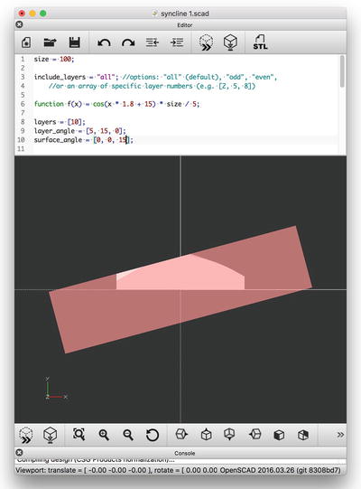
Figure 2-5. A single layer function rotated only about the z-axis. View is of the x-y plane.
Notice that the layers are first rotated through layer_angle and then cut off by the intersection of the box tilted at surface_angle. If this is too confusing, you might just experiment with different combinations one at a time to see the result in OpenSCAD’s preview mode.
A flag, include_layers, which determines whether to print the odd-numbered layers, even-numbered ones, all the layers, or an arbitrary set of layers. This allows for printing different layers in different colors if desired, as we have in this chapter.
Note
Geologists like to think in terms of dip and dip direction. Dip direction is represented in our model as the y value of the layer_angle variable if the z value is zero. Dip is the angle that the layer dips down relative to a horizontal surface. In our model this is the x value of the layer_angle variable, again if the z value is zero. There are good illustrations and a detailed description at https://en.wikipedia.org/wiki/Strike_and_dip . (There is another convention for orientation, strike and dip, which is less convenient for this model.) No component of surface_angle or layer_angle should exceed about 20 degrees to avoid printing issues.
Listing 2-1 creates an anticline with the surface layer partially “eroded” away (using the surface_angle variable) to make some of the layers visible (Figure 2-6). We show how to change the model to create a syncline in the next section of this chapter.

Figure 2-6. Anticline model—printed in two sets, one odd and one even
Tip
The models will not stay together very well just by stacking them. We folded blue masking tape back on itself to create little tubes, sticky side out, and stuck those between the layers. It is also easy to put the layers together incorrectly; be sure to keep track of the order of the pieces and which way around they go. If you forget, remember that the top and bottom surfaces of a print (in the orientation that they were printed) are usually easy to distinguish from one another.
Listing 2-1. OpenSCAD Anticline Model
// File anticline.scad// An OpenSCAD model of synclines and anticlines// The program defines a function for the middle layer and then// Defines layer thicknesses and offsets from this middle.// Rich "Whosawhatsis" Cameron, November 2016// Units: lengths in mm, angles in degrees, per OpenSCAD conventionssize = 100; //The dimension of the model in x and y, in mminclude_layers = "all"; //options: "all", "odd", "even",//or an array of specific layer numbers (e.g. [2, 5, 8])// Function that defines shape of center curvefunction f(x) = cos(x * 1.5 + 30) * size / 5;// offset of layer boundaries, relative to center curvelayers = [-20, -10, -6, 2, 10, 14, 22];// Thickness of each layer = difference between subsequent offsetslayer_angle = [5, 15, 0];// Vector of angles [x, y, z] rotating the curve relative to axessurface_angle = [10, 0, 0];// Vecto of angles about [x, y, z] to create sloping surface (top)// Use to expose lower layers// First create list of which layers to render// (odd, even, all, or specific ones)for(i = [0:len(layers) - 1]) if(((include_layers == "odd") && (i % 2))||((include_layers == "even") && !(i % 2))||(include_layers == "all")||len(search(i, include_layers))) translate([0, i*5, 0]) intersection() {// Now create the layers and rotate them appropriately// And intersect them with two bounding boxes defined below// To cut off a clean flat bottom surfacetranslate([-size / 2, 0, -size / 2]) cube([size, size, size]);rotate(surface_angle)cube([size * 2, size * .5, size * 2], center = true);rotate(layer_angle) linear_extrude(height = size * 2,center = true,convexity = 10) {difference() {offset(layers[i]) layer();if(i) offset(layers[i - 1] + .2) layer();}}}//Function to make polygons out of curvesmodule layer() polygon(concat([for(i = [-size:size]) [i, f(i)]],[[size, -size],[-size, -size]]));//End model
Printing a Syncline
Listing 2-1 creates the anticline shown in Figure 2-6. To create a syncline, we changed some of the parameters and also decided to make the models a little smaller (by changing the size parameter) because we found the models were taking a long time. Note that simply scaling the whole model is tricky because the layers might get too thin. You really need to think through the parameters to change. The changes to Listing 2-1 are the following:
size = 80;function f(x) = -cos(x * 1.8 + 15) * size / 5 + 30;layers = [-22, -10, -3, 5, 13, 22];layer_angle = [5, 15, 0];surface_angle = [12, 0, 0];
The resulting syncline is shown in Figure 2-7. Notice that this is not just the negative of the anticline function. The model is created by first creating the layers, rotating them if applicable, and then intersecting the model with a cube to cut off a flat bottom surface. Given that f(x) would go negative without the +30 term, the result of this operation would be that there would be very little left, as you can see in the OpenSCAD screenshot in Figure 2-8. (The model gives an exploded view of the layers. You can see that many of the layers would just be little unprintable scraps.)
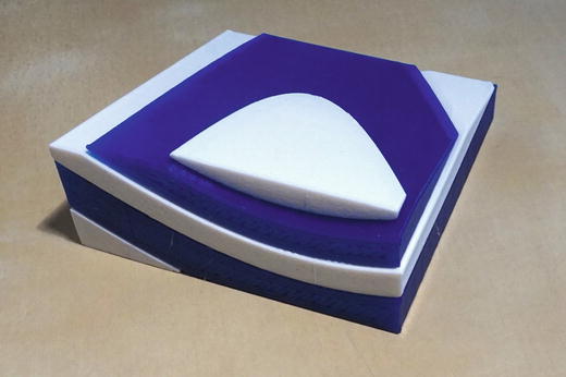
Figure 2-7. The syncline model
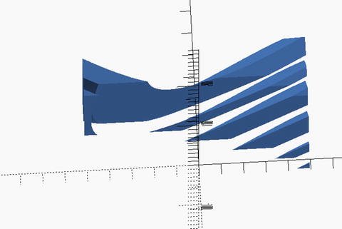
Figure 2-8. The syncline model without the offset term , visualized in OpenSCAD
Printing Tips for Syncline/Anticline Models
This model requires some degree of trial and error. Usually we try to have our prints be fairly foolproof, but in this case unless you use our examples as-is, you will need to look carefully at the pieces to be printed to be sure that they are not too small to be printed, too weirdly shaped, or not attached to the platform. Figures 2-9 and 2-10 show the odd and even pieces for the syncline model.
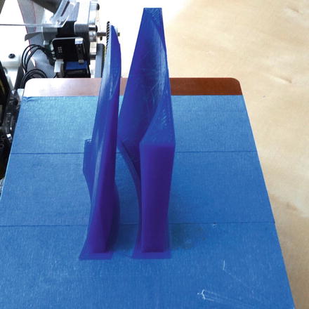
Figure 2-9. Half of the syncline model in Figure 2-5 on the printer

Figure 2-10. The other half of the syncline model
We recommend using a brim with these prints. A brim is a few loops on the platform around the base of a model, like the brim of a hat, which helps the model stick to the platform. You can see one in Figure 2-9. In some software, it may be called a “skirt” that is zero distance from the object.
Tip
In some circumstances you may want to use your printer program’s “ungroup” capability to turn one or more of the pieces to a more printable direction. In some cases, in the output STL from OpenSCAD, pieces may be suspended in mid-air. They will need to be brought down to the 3D printer’s platform and likely reoriented (180 degrees around the y-axis) in the program that you use to set up a print job (such as MatterControl, Cura, Repetier Host, or Makerbot Desktop).
In OpenSCAD, you may also want to add an offset term in the function f(x) to move the center layer up or down in the y direction as we do in the syncline model. Or you may use the surface_angle or layer_angle parameters to get rid of small corner pieces by cutting off some of the upper surface. Using OpenSCAD’s preview mode (see Appendix A) may be very helpful here.
The intent of this model is to help you gain insight into what formations look like when they have been squeezed, twisted, and then cut off at varying angles. It is important to remember that there is no geology knowledge encoded here and that this is purely a geometrical model. You may see physically inaccurate results if, for example, you make the amplitude of f(x) very much higher than we have it in our sample code or if you increase the frequency of the sinusoid represented by f(x) significantly. You will get results, but whether they are printable or represent a plausible formation is not possible to know in general.
3D Printing Terrain
The other way to get 3D printed models of interesting geological formations is to create them from one of the digital elevation databases that are available. The program we are partial to is Terrain2STL , developed by Thatcher Chamberlain. It is free and available at http://jthatch.com/Terrain2STL/ . The website says it is based on a database with a resolution of 90 meters per pixel at the equator.
If you want to get a bit more out there still, Chamberlain’s site also has an equivalent program for the Moon at http://jthatch.com/Moon2STL/ . The site states that the moon data has a bit under 2 km per pixel resolution at the Moon’s equator.
Figure 2-11 shows a print of the Rogue Valley area near Ashland, Oregon, from Terrain2STL. The program allows a user to select a region and how much to zoom in, and also allows the user to specify the vertical exaggeration. We often print out a “you are here” map of an area when we do an event. We are always amazed at how excited people get by it, and how much more insight you can gain from one than you can from a paper topographic map.

Figure 2-11. Oregon’s Rogue Valley (around Ashland), vertical scale exaggerated about ten times
Dunes
The models in the first section of this chapter were about geological formations that evolve very slowly, on time scales that make a human lifetime seem less than a blink. We will close this chapter with a model of far more ephemeral phenomena: sand dunes.
Sand dunes are piles of sand that form and re-form driven by the wind. Some types of dunes are stationary (forming around an outcropping of rock or some vegetation), but the ones we talk about here often migrate across long distances. In particular, barchan dunes often form large fields like the one shown in Figure 2-12. These dunes are crescent-shaped, with the nose of the dune pointed into the wind and long trailing horns on the downwind side. Wind would be blowing from the top of the picture towards the bottom in Figure 2-12. The darker areas are soil and plants between the dunes. These areas are lower than the dunes. Barchans typically form in “sand-starved” areas, where there is not enough sand for very deep seas of standing piles of sand to form.

Figure 2-12. Compound barchan dune in a downwind area of the White Sands National Monument, New Mexico. Dunes and interdune spaces are of approximately equal extent (rotated 90 degrees from original). Courtesy of U.S. Geological Survey, Department of the Interior/USGS, www.sciencebase.gov/catalog/item/51dd88f3e4b0f72b4471c140
Dunes start to form when wind piles up sand a bit, and this pile then has other sand blown up against it. The sand piles up steeply on the side facing into the wind (pushed by the wind). The side away from the wind slides down at the angle of repose, the maximum angle that a pile of loose material can sustain in a stable way. Figure 2-13 shows the details of this crest, where the slope pushed up by the wind meets the lee slope where material will slide down at the angle of repose, creating a relatively sharp curved edge along the top of the dune. The entire dune will march across the desert, progressing like a single wave on the sea.
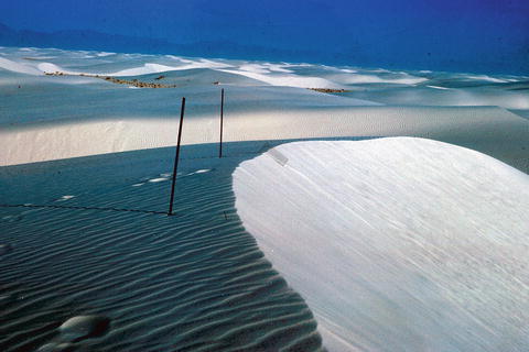
Figure 2-13. White Sands National Monument, New Mexico. Crest of barchan dune (wind blowing from left to right). Photo by J.R. Douglass, U.S. National Park Service, 1964. Courtesy of U.S. Geological Survey, Department of the Interior/USGS, www.sciencebase.gov/catalog/item/51dd894ee4b0f72b4471c19a
The Model
There are many mathematical models of the formation of sand dunes. Typically they model the statistical behavior of many sand grains to create a simulation of the flow of dunes across a space. The classic book in this field (originally published in 1941) is R. A. Bagnold ’s The Physics of Blown Sand and Desert Dunes (reissued by Courier Corporation, 2005). However, this was way beyond the scope of our book. As with the folded-rock models, we wanted to “3D surface fit” data to reproduce the basic shape of a dune while retaining as much of the physics as possible. Figure 2-14 shows the resulting 3D print.

Figure 2-14. Barchan dune model
There are three different parabolic curves used to create the 3D surface fit of this model, shown in full in Listing 2-2. The base of the windward side of the dune (the left side in Figure 2-12) is modeled by the first parabola which depends on the variables height , width, and length of the dune. length is the distance along the centerline from nose to tips of the crescent, and width is the distance between the two tips of the crescent.
The second parabola is the symmetrical dune cross-section , the pink structures in Figures 2-15 and 2-16. The angle of the windward side to the horizontal (typicallly 15 degrees, according to Bagnold and other sources) is the variable windward, and the angle of repose is the variable repose , typically 30 degrees for sand. These cross-sections depend on the angle windward and the variable height. These are offset so that the one end of each cross-section falls along the first parabola that forms the windward edge. All these cross-sections are the same as each other and are not rotated to follow the windward edge parabola, as is clear in Figures 2-15 and 2-16.

Figure 2-15. Barchan dune model cross-sections (pink) lined up along the parabola that forms the windward base of the dune
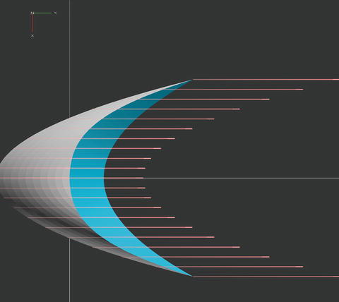
Figure 2-16. The cross sections in 2-15 viewed from above
To create the lee side, a set of rectangles (Figures 2-17 and 2-18) is generated along a third, leeward edge parabola. This leeward parabola is specified by all the same variables as the first parabola, plus the height and the two specified angles. Figure 2-18 shows these rectangles from above.
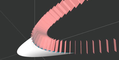
Figure 2-17. The rectangles that define the lee face of the dune

Figure 2-18. The rectangles in 2-17 from above
Finally, two surfaces are created using OpenSCAD’s hull() function, one that will create the windward side and one that will be subtracted from the windward side to create the lee slope. Loosely speaking, the hull() function creates the smallest possible convex shape that includes all the points you ask the hull() function to combine. The first hull across the cross-sections creates the windward side. Then a second surface is created by using the hull() fuction on the rectangles forming the lee side. The lee side is then subtracted from the windward side to give the final dune shape.
Printing the Dune Model
The barchan dune model is easy to print for just about any reasonable value of angle of repose and windward angle. It should not be necessary to use support or a brim—after all, the shape can be generated by wind blowing around sand, so the dunes are “additively manufactured” in real life.
Caution
This model takes a while to render in OpenSCAD—you may need to leave it running for a while before your model appears. See Appendix A (or the OpenSCAD manual) for how to use “preview” instead of full rendering.
Listing 2-2. Barchan Dune OpenSCAD Model
// File barchan.scad// An OpenSCAD model of barchan sand dunes// The program defines a parabola for the envelope// Based on the parameters at the top of the file.// Rich "Whosawhatsis" Cameron, November 2016// Units: lengths in mm, angles in degrees, per OpenSCAD conventionsheight = 10; // max height in z, mmwindward = 15; // angle to the horizontal of the nose of the dunerepose = 30; // angle of repose, degreeswidth = 100; // width at widest point (ends of crescent), mmlength = 100; // length from nose to center of crescent ends, mm// First create cross sections of the dune in the vertical plane// parallel to the wind direction// These cross sections are offset by a parabola// The back of the cross section, defined by angle of repose// for now, is symmetrical to the front// Later on we will subtract (difference) a cutoff at the angle of// reposedifference() {for(i = [-width/2:width/2 - 1])hull() for(i = [i, i + 1])translate([i, pow(i/width * 2, 2) * length, 0])rotate([90, 0, 90])linear_extrude(height = .001, scale = .001)polygon([for(i = [-1:.1:1])height * [i / tan(windward), 1 - i * i]]);// The next section creates the surface that we will subtract// from the windward side to create the angle of repose// on the leeward sidehull() for(i = [-width:width]) {translate([i,height / tan(repose) + (length - height / tan(repose) -height / tan(windward)) / pow(width / 2, 2) * pow(i, 2),0]) {rotate([90,0,90 + atan(2 * i * (length - height / tan(repose) -height / tan(windward)) / pow(width / 2, 2))// The previous line calculates the normal to the lee face parabola.]) {linear_extrude(height = .001, scale = 1) {rotate(90 - repose) translate([0, -1, 0]) square((height + 2) / sin(repose));} // end linear_extrude} // end rotate} // end translate} // end hull} // end difference// (subtracting the leeward face cutout from the rest of the model)
Barchan Dunes Beyond Earth
Barchan dunes have been spotted elsewhere in the solar system including on Mars and on Saturn’s moon Titan. Figure 2-19 shows these dunes on Mars. On Mars, though, the mechanism is a little different than on Earth, and thus the shape is different. Some scientists postulate that the dunes are stretched out because they are partially frozen some of the year, and the frozen nose of the dune does not move the way one would expect a dune on Earth to migrate, so the dune stretches out in one dimension or another. V. Schatz, H. Tsoar, K. S. Edgett, E. J. R. Parteli, and H. J. Herrmann postulated this in their Journal of Geophysical Research paper, “Evidence for indurated sand dunes in the Martian north polar region,” 28 April 2006.
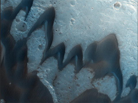
Figure 2-19. Image of barchan dunes on Mars from the High Resolution Imaging Science Experiment (HiRISE) on the Mars Reconnaisance Orbiter. Distance between the two horns of the merging dune is a bit over 500 meters. NASA/JPL/University of Arizona, www.uahirise.org/ESP_014404_1765
Not a lot is known about dunes on other worlds yet. There is not yet enough data, for example, to know whether barchan dunes on Mars migrate. There are also conflicting opinions in the scientific literature about the correct angle of repose to use. HiRISE scientist Nathan Bridges wrote a summary of aeolian processes on Mars and Titan that is a good snapshot of ongoing research: www.planetary.org/blogs/guest-blogs/2015/0326-lpsc-2015-aeolian-processes-mars-titan.html .
Note
Because the shape of a barchan dune on Mars and Titan is so much different from that of one on Earth, the model we have created for Earth dunes does not readily change to support the extraterrestrial versions.
Where to Learn More
The topics in this chapter would commonly be taught in an undergraduate class in physical geology. Our go-to reference was the textbook by W. K. Hamblin and E. H. Christiansen, Earth’s Dynamic Systems, 9th Edition (Prentice-Hall, 2001). If you want more easy-to-interpret sketches about geological formations, you may like David Lambert and the Diagram Group’s book The Field Guide to Geology (Facts on File, 1998).
The U.S. Geological Survey’s education site ( http://education.usgs.gov ) has fact sheets and links to resources at a variety of different levels. The U.S. National Park Service also has resources online about the geology of national parks; we enjoyed the writeup on types of dunes at www.nps.gov/grsa/learn/nature/dune-types.htm .
The geology of southern England is complex, and many fine examples can be found there of folded and uplifted rock. The Geological Society’s website ( www.geolsoc.org.uk ) is another treasure trove of imagery and descriptions of interesting formations.
Barchan and other dune formations on other planets are mostly described in the peer-reviewed scientific literature at this point, which can be heavy reading and may not be easily accessible. For example, possible barchans on Saturn’s moon Titan are described in a Nature Geoscience paper by R. C. Ewing, A. G. Hayes, and A. Lucas, “Sand dune patterns on Titan controlled by long-term climate cycles,” 8 December 2014. But if you search on the phrase “barchan dune,” you can find examples and photos of dunes on Earth and beyond and descriptions of the various models for their dynamics. You can also search on “aeolian processes” to learn about related phenomena.
Teaching with These Models
The initial trigger for this chapter was Joan’s husband (a British expat) musing about how nice it would have been to have had 3D printed models when he was studying geology of the south of England. It is complex to infer from the eroded surface what might lie beneath. The most straightforward way to use these models in education is to print a few that demonstrate the structure you are trying to study. One option might be to create a layered model of an underground or partially exposed formation and also print the terrain above it, as described in the sidebar “3D Printing Terrain.”
If you are a K-12 teacher, 3D printed models might be appropriate companions to having students create syncline and anticline clay models, as shown on paleontologist Jim Lehane’s site ( http://jazinator.blogspot.com/2010/05/teaching-folds-using-play-doh.html ). This site also has a lot of other links for K-12 teachers, including worksheets tied to movies that have incorrect depictions of geology. Teaching about Earth science standards, such as “Earth’s Systems” ( www.nextgenscience.org/pe/ms-ess2-2-earths-systems ), might benefit from these models.
Project Ideas
The most obvious way to use the layered-rock models is to create one that mimics a real formation or create a hypothetical one for discussions. If you want to make an elaborate model, you can make it in sections, but you will have to think hard about how to change the function for the middle layer and any rotations.
The barchan model is a little bit more of a one-off curiousity, but you might play with some of the variables like the angle of repose and see how this model changes. Angle of repose is dependent on the properties of the sand or other granular materials, and the shape of the lee side of the dune will change because of this. Results should be taken with a grain of salt (or maybe sand?) because this model does not really capture the interactions between the windward and lee sides of the dune, other than making some simple geometrical assumptions.
You can also think of the barchan as a case study of how to “surface fit” something based loosely on its physics plus its geometry, a situation that might come up more often than just in models of ephemeral sand phenomena.
Summary
This chapter shows how to create models of two types of geological formations. The first model allows you to create visualizations of layered rock formations similar to those found in many parts of the world where sedimentary rock is compressed and squeezed or uplifted. The second model is a 3D surface fit of a barchan dune, a particular type of dune that occurs in areas without a lot of sand. The model is tuned for barchan dunes on Earth, but these dunes are also found on Mars and possibly on Saturn’s moon Titan. The chapter also notes other available software for printing terrain and some ways to use the models.