
Water has some pretty weird properties. For example, it expands as it freezes; most other substances contract as they freeze. In this chapter we talk about ice and snow and create models of some of the more intriguing geometries that frozen water can create.
Water Ice
Figure 3-1 shows a familiar sight: an ice cube floating in water . The density of ice is 0.9167 grams per cubic centimeter at the freezing point; water at the same temperature is 0.9998 grams per cubic centimeter. If you add salt to the water (as we did in the cup of water in Figure 3-1), the saltwater becomes even denser. To make it roughly the same as seawater, add about a teaspoon and a half of table salt (8 grams) to 1 cup of water ( https://en.wikipedia.org/wiki/Salt ).
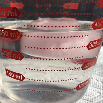
Figure 3-1. Fresh water ice in salt water
In the little experiment shown in Figure 3-1, a few drops of juice were added to the ice to make it more visible. Saltwater has a density of about 1.025 grams per cubic centimeter. We would expect about 10% of the volume of the ice to be above water in this case, because of the relative densities of ice and the liquid water it is floating in. Water expands as it freezes because it creates a crystal lattice of hexagons (Figure 3-2). Water molecules consist of two hydrogen atoms and an oxygen atom. When water freezes, each water molecule connects to four others in a roughly tetrahedral structure. In this chapter we explore the visible effects of that structure.
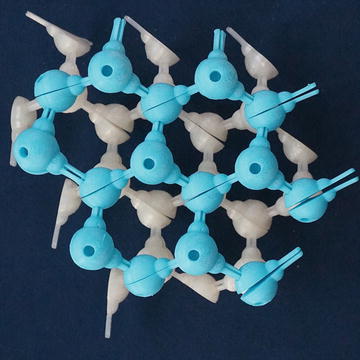
Figure 3-2. Molecular structure of an ice crystal
Note
We developed the 3D-printable, molecular-level model of ice crystals in Figure 3-2 in our previous 3D Printed Science Projects book (Apress, 2016, Chapter 7, “Molecules”). The larger spheres represent oxygen atoms; the smaller half-spheres between these spheres, hydrogen atoms. Each molecule in the lattice is connected to four others. Each oxygen has two hydrogens and two holes for connecting other oxygen atoms’ hydrogens. There are different ways the atoms can be connected to each other in hexagons. This one is called ice 1c.
Icebergs
Among the more intriguing results of the properties of freezing water are icebergs, giant floating mountains of ice. Typically they calve (split off) from glaciers to be carried around by currents until eventually they melt and erode away. Because they come from glaciers on land, fed by snow, icebergs are made of freshwater, not frozen ocean water. This fact has led some to suggest towing them to parched regions, like Southern California or Saudi Arabia, but as of this writing no one has pulled that off.
The fact that ice is 10% lighter than an equal volume of liquid water means that icebergs are about 90% submerged. As noted earlier in the chapter, seawater is a little denser still than freshwater, and makes a small additional difference (about 3.5% for the saltwater we created at the beginning of the chapter).
Icebergs represent famous hazards to navigation; the best-known example is the sinking of the Titanic when it struck an iceberg on its maiden voyage in 1912. Icebergs can pitch over, roll, or oscillate as they melt or as pieces break off and become unstable, which can be an even more serious hazard to any nearby ships. You can see this for yourself in a spectacular YouTube video from the Weather Channel at https://youtu.be/mvQ4eDKf9UY , or search YouTube for “rolling iceberg.”
Tabular icebergs split off from glaciers as thick slabs of ice, often with some less-compacted snow on top. Some of these icebergs can be huge. Iceberg B-15 calved from the Ross Ice Shelf in Antarctica in March 2000. It was 295 kilometers by 37 kilometres wide; recognizable pieces of it were detected for five years. By the time you read this, the Larsen C Ice Shelf in Antartica may have split along a deep rift that formed in 2016 and created an iceberg that, temporarily at least, will be about half the size of B-15.
The Model
We have developed a model of a tabular iceberg to visualize the above-water and below-water sections of an iceberg. Because icebergs come in all sorts of shapes and sizes, we decided to create two different sample models: one that is fundamentally a cylinder (with a variable radius) and another that is a frustrum of a cone (a cone with the top cut off).
Cylindrical Iceberg
Our first iceberg model is a cylinder , modified to have a variable radius. It is shown in Figure 3-3. The fine line near the top is the waterline (90% of the volume). In the open ocean, the part above that line would be the only part visible. The model allows you to set the height and the radius and to change the parameters featuresize, noise, and smoothness to respectively change how big the departures from a circle are, how many of them there are, and how much they have been smoothed out. Then the model extrudes this wavy-circle base straight up into a wavy cylinder. The model is given in Listing 3-1.

Figure 3-3. Cylindrical iceberg, with 10% volume line near top
Listing 3-1. The Cylindrical Iceberg
// File CylindricalIceberg.scad// An OpenSCAD model of an iceberg// Rich "Whosawhatsis" Cameron, January 2017height = 30; // height overall, in mmradius = 40; // maximum radiusfeaturesize = 20; // maximum variation from of radiusnoise = 10; // frequency of variations in radiussmoothness = 2; // how much to smooth the variationsseed = 0; // seed for random number generatorlinedepth = .2; // should be about half of your nozzle diameterpercentDistance = .9; // location of the water line$fs = .5;$fa = 2;// extrude the wavy outline and subtract the water linedifference() {union() {linear_extrude(height, convexity = 5) outline();if(linedepth < 0)translate([0, 0, height * percentDistance])linear_extrude(.5, center = true, convexity = 5)offset(-linedepth) outline();}if(linedepth > 0)translate([0, 0, height * percentDistance])linear_extrude(.5, center = true, convexity = 5)difference() {offset (2) outline();offset(-linedepth) outline();}}module outline() offset(-smoothness) offset(smoothness * 2)offset(-smoothness) polygon([for(theta = [0:noise:359],r = rands(radius, radius - featuresize, 1, seed + theta)) rect(r, theta)]);function rect(r, theta) = r * [sin(theta), cos(theta)];// End of model
Frustrum Iceberg
For our second model, we based our shape on the frustrum of a cone (a cone with the top cut off). As with the cylinder, we made the radius of the cone vary randomly. To solve this in general is very complicated. As is often the case for engineering problems, you can often vastly simplify things by changing just one of many parameters. In this case, we fixed the ratio of the size of the top of the iceberg to the bottom.
Even with this simplification, though, it takes a bit of geometry to figure out where the line of 10% volume falls. Figure 3-4 shows how we set up the problem. The blue (bottom) frustrum of the cone is in two parts: one that is 10% of the volume (on top) and one that is 90% (which will be below water in the real thing).
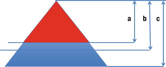
Figure 3-4. The geometry of the frustrum iceberg model
To make the math relatively tidy, we made a simplifying assumption that the frustrum was half the volume of a cone that includes the red (top) cone and the blue (bottom) frustrum, or a cone of height c in Figure 3-4. In other words, the red (top) cone is a cone that has the same volume as the blue frustrum.
It turns out that by thinking of the cones of height a, b, and c as all being similar (having the same angle at the top), you can show yourself that the volume of the cone of heights a, b, and c vary by the cube root of the height, because the radius will vary linearly with the height, and the area of the base goes as the square of the radius.
We know that the volume of a cone is one-third the area of the base times the height. So if we want to have the volume of the cone of height c be twice that of the red (top) cone, c will have to equal the cube root of 2 (which is about 1.2599) times the height a.
For the frustrum section between a and b to be 10% of the volume between lines a and c, b has to be the cube root of 1.1 (which is 1.0322) times a. The red (top) cone is just a convenience to help think about the geometry. All we want is the percentage difference between b and c so we know where the waterline is. Because we “throw away” the upper cone, we can have arbitrary values for the height and width of the frustrum, and the relationship will still hold. We will want the 10% line, then, to be at (c – b ) / ( c – a), or (1.2599 – 1.0322) / (1.2599 – 1) = 87.6% of the way from the bottom to the top.
Finally, based on Cavalieri’s Principle ( https://en.wikipedia.org/wiki/Cavalieri's_principle ), we can argue that as long as the curve we use for the base is extruded consistently from bottom to top, this holds for our wavy frustrum too. The result of all that math is shown in Figure 3-5 and the OpenSCAD model in Listing 3-2. The indented line would be the water line (at height b in Figure 3-4).
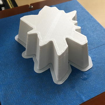
Figure 3-5. The frustrum iceberg model on a 3D printer
Listing 3-2. The Frustrum Iceberg Model
// File FrustrumIceberg.scad// An OpenSCAD model of an iceberg// Rich "Whosawhatsis" Cameron, January 2017height = 30; // height overall, in mmradius = 40; // maximum radiusfeaturesize = 20; // maximum variation from of radiusnoise = 10; // frequency of variations in radiussmoothness = 2; // how much to smooth the variationsseed = 0; // seed for random number generatorlinedepth = .2; // should be about half of your nozzle diameterCRRadius = pow(1.1, 1/3); //cube root of 1.1CR2 = pow (2, 1/3); // cube root of 2// calculate the location of the water linepercentDistance = (CR2 - CRRadius) / (CR2 -1);topScale = 1/CR2; // scale of top of frustrum relative to base$fs = .5;$fa = 2;// extrude the wavy outline with the top scalled and// subtract the water line at the height calculated abovedifference() {union() {linear_extrude(height, scale = topScale, convexity = 5)outline();if(linedepth < 0) intersection() {translate([0, 0, height * percentDistance])cube([radius * 10, radius * 10, .5],center = true);linear_extrude(height, scale = topScale, convexity = 5)offset(-linedepth) outline();}}if(linedepth > 0) intersection() {translate([0, 0, height * percentDistance])cube([radius * 10, radius * 10, .5], center = true);linear_extrude(height, scale = topScale, convexity = 5)difference() {offset(2) outline();offset(-linedepth) outline();}}}module outline() offset(-smoothness) offset(smoothness * 2)offset(-smoothness) polygon([for(theta = [0:noise:359],r = rands(radius, radius - featuresize, 1, seed + theta)) rect(r, theta)]);function rect(r, theta) = r * [sin(theta), cos(theta)];// End of model
Printing and Changing the Model
The model allows you to set the height and the radius and to change the parameters featuresize, noise, and smoothness to respectively change how big the departures from a right circular cone are, how many of them there are, and whether they have been smoothed out.
Because the indentation is a delicate feature, you may need to play with different slicing settings or even programs for best results.
Floating the Iceberg
It is tempting to try to float the iceberg model. However, because your prints will not be solid, we cannot give you a guaranteed reproducable way to have the iceberg float at a particular percentage of its volume. However, here are some useful numbers in case you want to try to make it work: PLA (the commonest plastic used in consumer 3D printers) is around 1.25 grams per cubic centimeter.
A 3D print will require you to set a value for infill (what percentage of the print is filled in with plastic, versus the volume being left full of air). We printed ours at 20% infill. In addition, the boundary of the object is solid plastic—let’s call that another 5%. Thus the average density of our print (air plus plastic) will be around 25% of 1.25, or 0.313. Water is just below 1 gram per cubic centimeter, as we noted earlier, so our print should be around 31% submerged. As you can see in Figure 3-6, it looks pretty close to that.

Figure 3-6. The PLA iceberg afloat in tap water
We can see that to get to 90% submerged we would have to go to 65% or so infill, plus the 5% perimeter, or 70% times the 1.25 density. That would eat a lot of time and filament, so you probably don’t want to create an accurately floating iceberg this way. If your printer uses ABS, that material has a density of only 1.05 grams per cubic centimeter, so you would need to use about 85% or so infill to be 90% submerged.
Vase Printing
You can also vase print your model. This means that you print a base and sides, but no top. Many slicers have a “spiral vase” option, and most others can be explicitly configured to print 0% infill and 0 solid layers on top, which has a similar effect. In MatterControl (see Appendix A), this setting is under Settings ➤ General ➤ Single Print ➤ Spiral Vase (with a box to select).
If you have vase prints, you can experiment with filling them 90% full of water (Figure 3-7). They should ride just a bit below the surface because of the heavier PLA displacing a bit more water. If you fill them 90% full of water, that is equivalent to filling them full of ice. Don’t try to freeze water in them, though, because the ice will likely break the PLA as it freezes and expands.
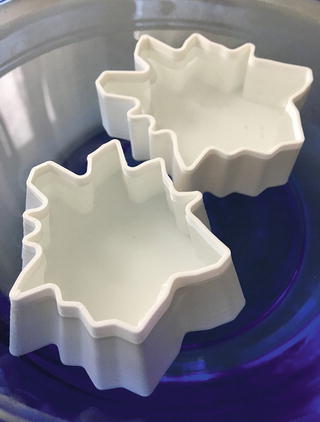
Figure 3-7. The two vase-printed icebergs in water
Snow
Water’s peculiar structure has many other implications, too. Snow has many of the properties it does because of the way snowflakes build up as they move though clouds. Snowflakes are crystals, too, always with six sides because of ice’s fundamental hexagonal structure. Creating an accurate model of snowflake formation is way beyond what we can sensibly do in this book. But we can come up with a simple model that you can then play with and see what structures result in the landscapes like the one in Figure 3-8.
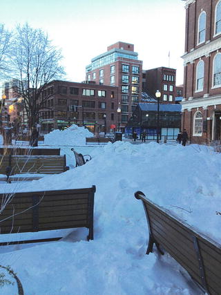
Figure 3-8. A snowy late winter afternoon in Boston
Physics of Snowflakes
Snowflakes are additively manufactured in clouds, but unlike 3D prints, they are not built up one layer at a time. Instead they accrete material in ways that depend on the conditions the flake encounters as it forms. Material is added mostly around the flake’s perimeter, rather than making the flake thicker. The temperature in the cloud and the excess water around at the time (called supersaturation) are the major determiners of what type of snowflake you will get.
The Snow Crystal Morphology diagram—sometimes called the Nakaya diagram , for 1930s physicist Ukichiro Nakaya —lays out what kinds of snowflakes form at various combinations of supersaturation and temperature. The Tip that follows lists some resources to find the details.
Tip
California Institute of Technology researcher Kenneth Libbrecht ’s book Field Guide to Snowflakes (Voyageur Press preprint, 2016) was a valuable resource that helped us think about the snowflake models, along with his website www.snowcrystals.com . It features pictures of and discussions about the physics of 21 different structures. The snowflake entry in Wikipedia is good too: https://en.wikipedia.org/wiki/Snowflake .
Our model here focuses on dendrites, the typical star-shaped snowflake form that you cut out of paper in third grade. These tend to form when the air is supersaturated and the temperatue is just below freezing (down to about –3.5 degrees Centigrade) or when the temperature is between –10 and –22 degrees Centigrade. Other than in those regimes, snowflakes can be solid plates or prisms, thick or thin, columns, and more, but always with the six-fold symmetry of the underlying crystal structure (except when two partially formed flakes merge).
Note
There are many 3D-printable snowflake models. One of the most ambitious is the Snowflake Machine ( www.thingiverse.com/thing:1159436 ) by Laura Taalman (a.k.a. Mathgrrl). This model (also in OpenSCAD) allows for many different variations of snowflakes with the Thingiverse Customizer.
The Model
The snowflakes we create here (like the one in Figure 3-9) will always be perfectly six-fold symmetrical (all six arms the same). Snowflakes in the wild are not always perfect, but we assume that here.
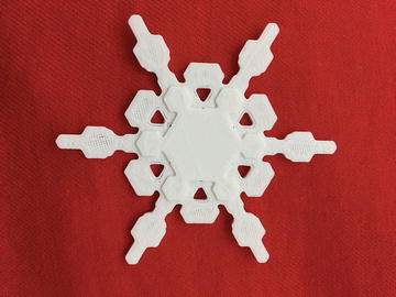
Figure 3-9. Snowflake model
The model (in Listing 3-3) works by creating randomly sized hexagonal pieces and accreting the smaller ones onto larger ones. The probability of the size and position of a given hexagonal addition is driven by OpenSCAD’s random number generator modified by a power law. You can change the parameter distribution in Listing 3-3 so that the size distribution of the hexagons being added follows the functions for cube, fifth power, and so on. The flake in Figure 3-9 was created with the default values of all the parameters in Listing 3-3.
Listing 3-3. Snowflake Model
// File snowflake.scad// An OpenSCAD model of an iceberg// Rich "Whosawhatsis" Cameron, January 2017// Units: lengths in mm, angles in degrees// per OpenSCAD conventionsmin = 2; // minimum size of a hexagon// should be large enough to print without breakingmax = 12; // maximum size of a hexagondistribution = 5; //exponent in power lawsmooth = .5; // smooth off edges// simulates snowflake, melting/sublimating a bitseed = 10; // seed for random number generator// same seed gives same resultiterations = 20; // how many times to add more hexagonslayer = 1; // how much smaller to make each layer than the lastminwidth = 0.5; // stops iterating branches if they get too// thin to print, which would result in disconnected sections$fs = .5;$fa = 2;// First create an array of random numbers skewed by power law// Random number is raised to the power "distribution"// and scaled by max-minarray = [for(v = rands(0, max - min, iterations, seed))min + pow(v, distribution) /pow(max - min, distribution - 1)];// Create six armsfor(i = [0:3]) linear_extrude(1 + i * .5)offset(smooth) offset(-smooth * 2) offset(smooth)for(a = [0:60:359]) rotate(a) grow(shrink = i * layer);// recursive function that grows each arm or branchmodule grow(n = 1, branch = true, shrink = 0) {// create one hexagoncircle(array[n] - shrink, $fn = 6);// then decide whether to continue with recursionif(n < len(array) && (array[n] - shrink) > minwidth) {translate([abs(array[n] - array[n + 1]) + 1 - shrink,0,0])grow(n + 1, branch, shrink);// branch if size has decreased sufficientlyif((array[n] - 2) > array[n + 1] && n > 5 && branch)for(a = [60, -60]) rotate(a)translate([abs(array[n] - array[n + 1]) + 1, 0, 0])grow(n + 1, false, shrink + 1);}}// End model
Printing and Changing the Model
The best way to explore the model is to play with the various parameters. The model creates hexagons with a random distribution of size, so the biggest effect can be changing the seed.This model can create dendrites and basic hexagonal shapes. Figure 3-10 shows some example flakes with a few parameters changed from the values in Listing 3-3. The one on the left has iterations = 10, making it stubbier and closer to a stellar plate type flake; the one in the middle has distribution = 10, seed = 3, and layer = 0.5; and the one on the right has layer = 0.5, seed = 3, and distribution = 15.

Figure 3-10. Snowflakes with different parameters, as described in the text
If you would like to make the more basic geometrical shapes (six-sided columns or prisms), Rich has posted a set of open source constant-geometry shapes on Youmagine that could get you started. You can find them at www.youmagine.com/designs/fixed-volume-objects .
Where to Learn More
The study of Arctic snow and ice has taken on a particular urgency in the light of climate change, which might cause large ice sheets to collapse into icebergs. You can look up the history of Antarctic ice sheets Larsen A, B, and C. Larsen A and B collapsed in 1995 and 2002, respectively. As we write in early 2017, Larsen C seems to be headed for the same fate. There is a summary at https://en.wikipedia.org/wiki/Larsen_Ice_Shelf . This is relevant to people far from Antarctica, because if these large ice sheets float away from Antarctica and melt, sea levels may begin to rise significantly. Understanding how and why ice sheets calve into icebergs and how long it takes for them to melt will be a key scientific endeavor in the coming years.
For more about snowflakes, as noted earlier, the work of Caltech’s Kenneth Libbrecht is a good and accessible source at the level of his general-public books and website already mentioned. He also has professional papers in this sphere, if you have access to scientific journals. Unfortunately, a lot of the math to fully simulate snowflake calculation is better suited to supercomputers—one has to bear in mind complicated interactions between the air, the forming snowflake, water vapor in the air, and so on. A good survey of current research can be found in Ron Cowan’s brief 2012 Scientific American article “Snowflake Growth Successfully Modeled from Physical Laws,” available online at www.scientificamerican.com/article/how-do-snowflakes-form .
Teaching with These Models
These models can be used to talk about ice and snow. But the approaches we use here in all the models of the chapter (of simplifying and using curve fits when the complexity is too high) can be used as a lesson as well. This aligns with the U.S. Next Generation Science Standards (NGSS) Engineering Technology and Application of Science (ETS2) Core Disciplinary Ideas about learning to break down a problem into solvable parts ( www.nextgenscience.org/dci-arrangement/hs-ps2-motion-and-stability-forces-and-interactions ). For example, we simplified the cone frustrum iceberg model significantly by fixing the ratio between the top and the bottom of the frustrum. Although this did not allow us to do every conceivable shape, it did allow the radius and height to be variable parameters.
Ice sheets collapsing into icebergs and how the freshwater in the icebergs is absorbed by the ocean may apply to earth science standards such as www.nextgenscience.org/pe/5-ess2-2-earths-systems , which looks at how freshwater and ocean water cycles interact.
Another concept we did not allude to directly in this chapter is the concept of finding volumes by displacement. Our calculation of how low any of the iceberg models should ride in the water could be used at several levels to talk about volumes of different solids, or Archimedes’ Principle ( https://en.wikipedia.org/wiki/Archimedes'_principle ), which says that a body floating on water will displace a volume of water equal to its mass. These discussions can fit into the motion and stability forces and interactions standards at various grade levels.
Project Ideas
These models can be used to think about the role of melting ice in sea level change, or perhaps to motivate and help think about studying the ocean currents that carry icebergs for long distances. Projects about displacement, volume, and other basics might be more interesting in the context of water ice sailing the seas than it might be in the abstract. There are also new ecosystems being discovered under ice shelves, and the effects of huge sheets of ice being ripped from above these areas would be an interesting project to explore as well. The Larsen ice sheet disintegrations resulted in some discoveries along these lines.
Because the models in this chapter do have significant simplifications of the physics they represent, good student projects (at a variety of levels) could look at improving and expanding the models, or perhaps creating simulation or experimental data that then could inform these models. For example, given how our simple snowflake accretion model works, could you add a parameter or a second level of detail that could give more physical and more interesting results? What might be good next steps from this model? In the more experimental sphere, one could create a version of the snowflake microscope suggested at the end of Libbrecht’s Field Guide to Snowflakes to take empirical data.
Summary
In this chapter we create models of icebergs and snowflakes. We also explore how icebergs calve from glaciers and then ride the seas 90% submerged as they erode and melt away. We discuss issues that arise when we want to model processes (like snowflake creation) that are too complex to model in detail with the tools available to us, and how to make reasonable engineering approximations. We also use Archimedes’ Principle to think about how substances with different densities will displace water proportionate to their mass, and not their volume.