Frequency Shift

The shifted frequency an observer hears from something moving toward them at a velocity v is determined by the equation

• Shifted frequency = (1 + v / a) * ( frequency at rest)

where a is the speed of sound . If the source of the sound is moving away, the frequency changes like this:

• Shifted frequency = (1 – v / a) * ( frequency at rest)

Think about the waves bunching up and getting closer together as the source moves toward you. The frequency rises as the distance between subsequent waves gets smaller.

The ratio of a moving object’s velocity to the speed of sound (the v / a term in the shifted frequency equation) is called the Mach number, commonly denoted by M. It is named in honor of Mach, but was not defined by him.

The speed of sound depends on the temperature of the air (or other gas) that is carrying the sound waves, and ambient density and pressure, all of which are interrelated. Warmer air will transmit the small physical disturbance of a sound wave from molecule to molecule faster. The molecules in hot, dense air are flying around faster and will more efficiently propagate a sound wave. For example, in the cold, thin air up where commercial airliners fly, at 10 kilometers (32,800 feet) above mean sea level, the speed of sound slows to 667 miles per hour from the 767 at sea level—a 13% decrease.

The Model

This model is based on the wave model in our earlier book 3D Printed Science Projects (Apress, 2016; Chapter 2, “Light and Other Waves”). That model ultimately needs to get a set of points to plot out a 3D surface. In this case, because the source is moving, we need to work backwards from a point in x and y and figure out what wave would be passing over that point at a particular time.

We think about this by imagining that we are taking a snapshot at one particular time of all the waves that have been generated by our moving point source since it came into our field of view. Imagine that as the point source was flying along it puffed out a smoke ring on a regular basis. The oldest smoke rings would be the biggest, and the new ones the smallest. Instead of single smoke rings, though, we imagine our source is putting out a cosine wave at a particular frequency.

The waves from the moving source are traveling at the speed of sound. So we know that a wave that arrives at a particular point was generated by a source that was at the center of that circle at a time in the past. We can calculate that time by dividing the radius of the circle by the speed of sound. Figure 4-3 shows this situation, and we will work through the math to show you how we got our equations. We want to find A, the radius from where the wave (now at point (x,y)) started back when the disturbance was at P1. We show the point where the source is now as (0,0).

Figure 4-3. Geometry to figure out which wave contributes to the amplitude at a particular point (x,y) at a particular snapshot in time

We think of the object flying from P1 to the current origin of its coordinate system in space, (0,0). We want to find the distance A in Figure 4-3 that is the distance of the posiition of the source when the wave was generated to the point (x,y).

We know the following to start with (based on the diagram in Figure 4-3):

• Our object creating the disturbance went from P1 to (0,0) moving at Mach number M.

• The radius from the current position to the point (x,y)—we call this R.

• The angle theta, which is the angle with tangent y / x.

• That the angles in a triangle sum to 180 degrees.

• That B / A equals the Mach number M since the object moved M times the speed of sound times the time while the disturbance (moving at the speed of sound) moved from P1 to (x,y).

To work out the math, we will use the law of sines, which says that for all the angles in a triangle, the ratios of the sine of all their angles to their opposite sides is equal. In this case, that would be:

• sin(theta) / A = sin(b) / B = sin(r) / R

Since we know that B/A = M, use the relationships between the first two sides to get:

• sin(theta) / A = sin(b) / MA (substituting MA for B)

Therefore, b = asin(M * sin(theta))

Next we need to get the third angle, r. Since the angles in a triangle add up to 180 degrees,

• 180 = theta + asin(M * sin(theta)) + r

or

• r = 180 – theta – asin(M * sin(theta))

Going back to the original law of sines, we know that the angles theta and r are related like this:

• sin(theta) / A = sin(r) / R

or

• A = sin (theta) * R / sin (r)

Finally, to get A (which is what we wanted all along) we plug in the values we have found to get:

• A = sin (theta) * R /

• sin (180 – theta – asin(M * sin(theta)))

This is a peak of the cosine wave that was generated at P1 in the past. The speed of the disturbance is Mach number times speed of sound. We are creating this whole snapshot at one (arbitrary) time, and so you can see that the actual values of time drop out in the algebra we just worked out.

Finally, we use that value of amplitude * cos(A*frequency) as the height of our wave at position (x,y) at our arbitrary time. Whew!

Listing 4-1. The Doppler Model

// File doppler.scad
// An OpenSCAD model of a snapshot of the waves
// around a moving object

// The model is based on the waves models in
// Volume 1 of 3D Printed Science Projects
// Rich "Whosawhatsis" Cameron, December 2016
// Units: lengths in mm, angles in degrees
// per OpenSCAD conventions
// This program creates a res*xmax mm by res*ymax rectangle
// As shown here will be 100 mm square.

// Model only valid for subsonic objects(mach < 1)

mach = .5; // mach number – must be less than 1.0
frequency = 20; // frequency - increase to show more waves
// setting frequency to high for the mach number will
// result in sampling artifacts
amplitude = .5; // Height of wave peaks on either side of the base plane, mm
thick = 2; // thickness of the slab, mm
xmax = 199; // max dimension in x (before scaling by res)
ymax = 199; //max dimension in x (before scaling by res)
res = .5; // scaling factor

// This function calculates a cosine wave with doppler shift:
function f(x, y) = amplitude * cos(r(x, y) / sin(theta(x, y) + asin(sin(theta(x, y)) * mach)) * sin(theta(x, y)) * frequency);

// These two functions convert x/y values to polar coordinates:
function r(x, y, center = [xmax/2, ymax/2]) = sqrt(pow(center[0] - x, 2) + pow(center[1] - y, 2));
function theta(x, y, center = [xmax/2, ymax/2]) = atan2((center[1] - y), (center[0] - x));

// The rest of the model is the same as the
// wave model in Volume 1.
// It creates and interpolates a surface z = f(x,y)
// 3D printer conventions are that z is vertical –
// The model is rotated at the end
// so that the (x, y) surface is vertical, not horizontal
// This gives better print quality and allows for a wave
// surface on both sides of a print
// without support

toppoints = (xmax + 1) * (ymax + 1);

center = [xmax/2, ymax / 2];

points = concat(
   // top face
   [for(y = [0:ymax], x = [0:xmax]) [x, y, f(x, y)]],
   (thick ? //bottom face
      [for(y = [0:ymax], x = [0:xmax]) [x, y, f(x, y) - thick]]
   :
      [for(y = [0:ymax], x = [0:xmax]) [x, y, 0]]
   )
);

zbounds = [
   min([for(i = points) i[2]]),
   max([for(i = points) i[2]])
];
function quad(a, b, c, d, r = false) = r ?
   [[a, b, c], [c, d, a]]:
   [[c, b, a], [a, d, c]]; //create triangles from quad

faces = concat(
   //build top and bottom
   [for(
      bottom = [0, toppoints],
      i = [for(x = [0:xmax - 1],
      y = [0:ymax - 1]
   )
      quad(
         x + (xmax + 1) * (y + 1) + bottom,
         x + (xmax + 1) * y + bottom,
         x + 1 + (xmax + 1) * y + bottom,
         x + 1 + (xmax + 1) * (y + 1) + bottom,
         bottom
      )], v = i) v],
   //build left and right
   [for(i = [for(x = [0, xmax], y = [0:ymax - 1])
      quad(
         x + (xmax + 1) * y + toppoints,
         x + (xmax + 1) * y,
         x + (xmax + 1) * (y + 1),
         x + (xmax + 1) * (y + 1) + toppoints,
         x
      )], v = i) v],
   //build front and back
   [for(i = [for(x = [0:xmax - 1], y = [0, ymax])
      quad(
         x + (xmax + 1) * y + toppoints,
         x + 1 + (xmax + 1) * y + toppoints,
         x + 1 + (xmax + 1) * y,
         x + (xmax + 1) * y,
         y
      )], v = i) v]
);

// prevent an incorrect model from being generated
if(1 > mach && mach > -1) {
   // Scale and rotate the print
   rotate([90, 0, 0]) scale([res, res, 1]) {
      polyhedron(points, faces);
   }
} else echo("mach number must be less than 1");
// end model

Printing and Changing the Model

As you saw in Figure 4-2, this model prints vertically—otherwise you would need to pick a lot of support off the model, and the waves would not print as cleanly. Because the model is very thin, we recommend against scaling it in your slicing software. Instead, change anything you want to in OpenSCAD. You can scale the model by changing the variable res, which multiplies the default size of 200 mm on a side (res = 0.5 gives you 100 mm square pieces).

You can change the variable frequency to change the frequency of the wave the moving object is creating. The variable mach is the Mach number, which should be less than 1 for this model.

Shock Waves

Imagine that a plane is flying supersonically and making noise. The noise it made a second ago will be spreading out in a sphere, but the plane will have punched through that outer spreading sphere and moved on before the sphere gets there. This creates a shock wave angled away from the nose of plane at the Mach angle, which is an angle with a sine that is the reciprocal of the Mach number. At Mach 3, this is asin(1 / 3), or about 19 degrees. The Mach cone’s front will be twice the Mach angle, which you can verify from our models.

The Model

Our 3D printed model is shown in Figure 4-4 for a subsonic (Mach 0.5), transonic (Mach 1), and supersonic (Mach 3) case in which the vehicle is flying to the right of the picture at a 30-degree angle from the vertical.

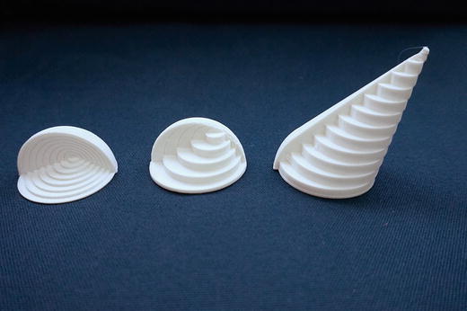
Figure 4-4. Mach cone models for Mach 0.5, 1, and 3

The model (Listing 4-2) is created by first making two spheres: one centered at the first modeled time with a radius that is the distance sound travels between that first modeled time and the current time, and a second sphere that is centered where the disturbance was just before its current position. OpenSCAD’s hull() function is used to create a surface that contains these spheres and all the intermediate ones. This creates a smooth surface away from the stair steps that shows what the outer boundary of the sound traveling away would look like. The stair steps are cuts through the diameter of spheres at regular intervals along the direction of travel.

Figure 4-5 shows a different view of this envelope of the edge of the propagating waves for a supersonic point source moving to the right of the picture. We have shown both the 2D propagation of the edge of the disturbance from the moving point source (the circles) and the surface that defines the edge of all the disturbances if we made the steps between circles smaller and smaller.

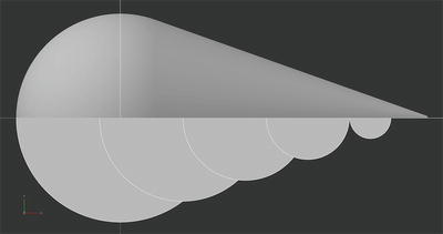
Figure 4-5. 2D projection of the Mach cone

Listing 4-2. The Mach Cone Model

// File machCone.scad
// An OpenSCAD model of a snapshot
// of the propagating disturbance
// From a point source moving at mach number, "mach"

// The model prints a disk that is a cross-section of
// the sphere representing a propagating disturbance
// from the traveling point source
// and a surface that is the envelope of
// the boundary of these propagating spheres
// Assumes point source at constant velocity

// Rich "Whosawhatsis" Cameron, December 2016
// Units: lengths in mm, angles in degrees,
// per OpenSCAD conventions

mach = 0.5; // mach number

size = 50; // diameter of the oldest propagation circle, in mm
a = 30; // angle from the vertical at which
// the point source is traveling
step = 3; // size of the circular cross-section steps

$fs = 2; // decrease this for smoother curves.
// This will slow down rendering.
$fa = 2;

// First section creates the outer boundary created by
// smoothing spheres of propagating
// disturbance as the point source moves
difference() {
   intersection() {
      hull() for(i = [1, size / 2]) {
        translate([sin(a), 0, cos(a)] * (size / 2 - i) * mach)
          sphere(r = i);
      }
      translate([-size, 0, 0]) cube(size * 10);
   }
   if(mach < = 1) for(i = [5:step:size / 2]) {
      translate([sin(a), 0, cos(a)] * (size / 2 - i) * mach) {
         rotate([90, 0, 0]) {
            linear_extrude(2, center = true) difference() {
               circle(i);
               circle(i - .2);
            }
         }
      }
   }
} // end difference

// Next create the stair steps representing the diameter of
// propagation circles
intersection() {
   for(i = [0:step:size / 2 + step]) {
      translate([sin(a), 0, cos(a)] * (size / 2 - i) * mach) {
         cylinder(
            r = i,
            h = step * mach * cos(a) + .01,
            center = true
         );
      }
   }
   translate([-size, -size * 10, 0]) cube(size * 10);
}

// end model

Printing and Changing the Model

As with the Doppler model, we suggest you do not scale this model down with your printer’s scaling; change anything you want to in the model itself by changing the variable size, which is the diameter of the largest (bottom) circle in mm. The variable mach is the Mach number. Scaling it up should work, although you may see some of the facets of the approximations making up the model if you scale it too much outside of OpenSCAD.