Features and Classifiers
Feature extraction and classification are two key stages of a typical computer vision system. In this chapter, we provide an introduction to these two steps: their importance and their design challenges for computer vision tasks.
Feature extraction methods can be divided into two different categories, namely hand-engineering-based methods and feature learning-based methods. Before going into the details of the feature learning algorithms in the subsequent chapters (i.e., Chapter 3, Chapter 4, Chapter 5, and Chapter 6), we introduce in this chapter some of the most popular traditional hand-engineered features (e.g., HOG [Triggs and Dalal, 2005], SIFT [Lowe, 2004], SURF [Bay et al., 2008]), and their limitations in details.
Classifiers can be divided into two groups, namely shallow and deep models. This chapter also introduces some well-known traditional classifiers (e.g., SVM [Cortes, 1995], RDF [Breiman, 2001, Quinlan, 1986]), which have a single learned layer and are therefore shallow models. The subsequent chapters (i.e., Chapter 3, Chapter 4, Chapter 5, and Chapter 6) cover the deep models, including CNNs, which have multiple hidden layers and, thus, can learn features at various levels of abstraction.
2.1 IMPORTANCE OF FEATURES AND CLASSIFIERS
The accuracy, robustness, and efficiency of a vision system are largely dependent on the quality of the image features and the classifiers. An ideal feature extractor would produce an image representation that makes the job of the classifier trivial (see Fig. 2.1). Conversely, unsophisticated features extractors require a “perfect” classifier to adequately perform the pattern recognition task. However, ideal features extraction and a perfect classification performance are often impossible. Thus, the goal is to extract informative and reliable features from the input images, in order to enable the development of a largely domain-independent theory of classification.
A feature is any distinctive aspect or characteristic which is used to solve a computational task related to a certain application. For example, given a face image, there is a variety of approaches to extract features, e.g., mean, variance, gradients, edges, geometric features, color features, etc.
The combination of n features can be represented as a n-dimensional vector, called a feature vector. The quality of a feature vector is dependent on its ability to discriminate image samples from different classes. Image samples from the same class should have similar feature values and images from different classes should have different feature values. For the example shown in Fig. 2.1, all cars shown in Fig. 2.2 should have similar feature vectors, irrespective of their models, sizes, positions in the images, etc. Thus, a good feature should be informative, invariant to noise and a set of transformations (e.g., rotation and translation), and fast to compute. For instance, features such as the number of wheels in the images, the number of doors in the images could help to classify the images into two different categories, namely “car” and “non-car.” However, extracting such features is a challenging problem in computer vision and machine learning.
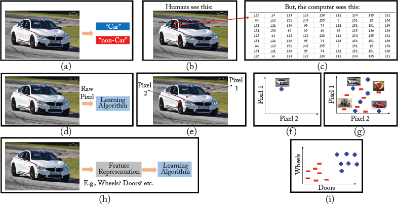
Figure 2.1: (a) The aim is to design an algorithm which classifies input images into two different categories: “Car” or “non-Car.” (b) Humans can easily see the car and categorize this image as “Car.” However, computers see pixel intensity values as shown in (c) for a small patch in the image. Computer vision methods process all pixel intensity values and classify the image. (d) The straightforward way is to feed the intensity values to the classifiers and the learned classifier will then perform the classification job. For better visualization, let us pick only two pixels, as shown in (e). Because pixel 1 is relatively bright and pixel 2 is relatively dark, that image has a position shown in blue plus sign in the plot shown in (f). By adding few positive and negative samples, the plot in (g) shows that the positive and negative samples are extremely jumbled together. So if this data is fed to a linear classifier, the subdivision of the feature space into two classes is not possible. (h) It turns out that a proper feature representation can overcome this problem. For example, using more informative features such as the number of wheels in the images, the number of doors in the images, the data looks like (i) and the images become much easier to classify.

Classification is at the heart of modern computer vision and pattern recognition. The task of the classifier is to use the feature vector to assign an image or region of interest (RoI) to a category. The degree of difficulty of the classification task depends on the variability in the feature values of images from the same category, relative to the difference between feature values of images from different categories. However, a perfect classification performance is often impossible. This is mainly due to the presence of noise (in the form of shadows, occlusions, perspective distortions, etc.), outliers (e.g., images from the category “buildings” might contain people, animal, building, or car category), ambiguity (e.g., the same rectangular shape could correspond to a table or a building window), the lack of labels, the availability of only small training samples, and the imbalance of positive/negative coverage in the training data samples. Thus, designing a classifier to make the best decision is a challenging task.
2.2 TRADITIONAL FEATURE DESCRIPTORS
Traditional (hand-engineered) feature extraction methods can be divided into two broad categories: global and local. The global feature extraction methods define a set of global features which effectively describe the entire image. Thus, the shape details are ignored. The global features are also not suitable for the recognition of partially occluded objects. On the other hand, the local feature extraction methods extract a local region around keypoints and, thus, can handle occlusion better [Bayramoglu and Alatan, 2010, Rahmani et al., 2014]. On that basis, the focus of this chapter is on local features/descriptors.
Various methods have been developed for detecting keypoints and constructing descriptors around them. For instance, local descriptors, such as HOG [Triggs and Dalal, 2005], SIFT [Lowe, 2004], SURF [Bay et al., 2008], FREAK [Alahi et al., 2012], ORB [Rublee et al., 2011], BRISK [Leutenegger et al., 2011], BRIEF [Calonder et al., 2010], and LIOP [Wang et al., 2011b] have been used in most computer vision applications. The considerable recent progress that has been achieved in the area of recognition is largely due to these features, e.g., optical flow estimation methods use orientation histograms to deal with large motions; image retrieval and structure from motion are based on SIFT descriptors. It is important to note that CNNs, which will be discussed in Chapter 4, are not that much different than the traditional hand-engineered features. The first layer in the CNNs learn to utilize gradients in a way that is similar to hand-engineered features such as HOG, SIFT and SURF. In order to have a better understanding of CNNs, we describe next, three important and widely used feature detectors and/or descriptors, namely HOG [Triggs and Dalal, 2005], SIFT [Lowe, 2004], and SURF [Bay et al., 2008] in some details. As you will see in Chapter 4, CNNs are also able to extract similar hand-engineered features (e.g., gradients) in their lower layers but through an automatic feature learning process.
2.2.1 HISTOGRAM OF ORIENTED GRADIENTS (HOG)
HOG [Triggs and Dalal, 2005] is a feature descriptor that is used to automatically detect objects from images. The HOG descriptor encodes the distribution of directions of gradients in localized portions of an image.
HOG features have been introduced by Triggs and Dalal [2005] who have studied the influence of several variants of HOG descriptors (R-HOG and C-HOG), with different gradient computation and normalization methods. The idea behind the HOG descriptors is that the object appearance and the shape within an image can be described by the histogram of edge directions. The implementation of these descriptors consists of the following four steps.
Gradient Computation
The first step is the computation of the gradient values. A 1D centered point discrete derivative mask is applied on an image in both the horizontal and vertical directions. Specifically, this method requires the filtering of the gray-scale image with the following filter kernels:
Thus, given an image I, the following convolution operations (denoted by *) result in the derivatives of the image I in the x and y directions:
Thus, the orientation θ and the magnitude |g| of the gradient are calculated as follows:

As you will see in Chapter 4, just like the HOG descriptor, CNNs also use convolution operations in their layers. However, the main difference is that instead of using hand-engineered filters, e.g., fx, fy in Eq. (2.1), CNNs use trainable filters which make them highly adaptive. That is why they can achieve high accuracy levels in most applications such as image recognition.
Cell Orientation Histogram
The second step is the calculation of the cell histograms. First, the image is divided into small (usually 8 × 8 pixels) cells. Each cell has a fixed number of gradient orientation bins, which are evenly spread over 0–180° or 0–360°, depending on whether the gradient is unsigned or signed. Each pixel within the cell casts a weighted vote for a gradient orientation bin based on the gradient magnitude at that pixel. For the vote weight, the pixel contribution can be the gradient magnitude, or the square root of the gradient magnitude or the square of the gradient magnitude.
Block Descriptor
To deal with changes in illumination and contrast, the gradient strengths are locally normalized by grouping the cells together into larger, spatially connected blocks. The HOG descriptor is then the vector of the components of the normalized cell histograms from all of the block regions.
Block Normalization
The final step is the normalization of the block descriptors. Let v be the non-normalized vector containing all histograms in a given block, ||v||k be its k-norm for k = 1, 2, and ϵ be a small constant. Then the normalization factor can be one of the following:

or

or

There is another normalization factor, L2-Hys, which is obtained by clipping the L2-norm of v (i.e., limiting the maximum values of v to 0.2) and then re-normalizing.
The final image/RoI descriptor is formed by concatenating all normalized block descriptors. The experimental results in Triggs and Dalal [2005] show that all four block normalization methods achieve a very significant improvement over the non-normalized one. Moreover, the L2-norm, L2-Hys, and L1-sqrt normalization approaches provide a similar performance, while the L1-norm provides a slightly less reliable performance.

Figure 2.3: HOG descriptor. Note that for better visualization, we only show the cell orientation histogram for four cells and a block descriptor corresponding to those four cells.
2.2.2 SCALE-INVARIANT FEATURE TRANSFORM (SIFT)
SIFT [Lowe, 2004] provides a set of features of an object that are are robust against object scaling and rotations. The SIFT algorithm consists of four main steps, which are discussed in the following subsections.
Scale-space Extrema Detection
The first step aims to identify potential keypoints that are invariant to scale and orientation. While several techniques can be used to detect keypoint locations in the scale-space, SIFT uses the Difference of Gaussians (DoG), which is obtained as the difference of Gaussian blurring of an image with two different scales, σ, one with scale k times the scale of the other, i.e., k × σ. This process is performed for different octaves of the image in the Gaussian Pyramid, as shown in Fig. 2.4a.
Then, the DoG images are searched for local extrema over all scales and image locations. For instance, a pixel in an image is compared with its eight neighbors in the current image as well as nine neighbors in the scale above and below, as shown in Fig. 2.4b. If it is the minimum or maximum of all these neighbors, then it is a potential keypoint. It means that a keypoint is best represented in that scale.

Figure 2.4: Scale-space feature detection using a sub-octave DoG pyramid. (a) Adjacent levels of a sub-octave Gaussian pyramid are subtracted to produce the DoG; and (b) extrema in the resulting 3D volume are detected by comparing a pixel to its 26 neighbors. (Figure from Lowe [2004], used with permission.)
Accurate Keypoint Localization
This step removes unstable points from the list of potential keypoints by finding those that have low contrast or are poorly localized on an edge. In order to reject low contrast keypoints, a Taylor series expansion of the scale space is computed to get more accurate locations of extrema, and if the intensity at each extrema is less than a threshold value, the keypoint is rejected.
Moreover, the DoG function has a strong response along the edges, which results in a large principal curvature across the edge but a small curvature in the perpendicular direction in the DoG function. In order to remove the keypoints located on an edge, the principal curvature at the keypoint is computed from a 2 × 2 Hessian matrix at the location and scale of the keypoint. If the ratio between the first and the second eigenvalues is greater than a threshold, the keypoint is rejected.
Remark: In mathematics, the Hessian matrix or Hessian is a square matrix of second-order partial derivatives of a scalar-valued function. Specifically, suppose f(x1, x2, …, xn) is a function outputting a scalar, i.e., ![]() ; if all the second partial derivatives of f exist and are continuous over the domain of the function, then the Hessian H of f is a square n × n matrix, defined as follows:
; if all the second partial derivatives of f exist and are continuous over the domain of the function, then the Hessian H of f is a square n × n matrix, defined as follows:

Orientation Assignment
In order to achieve invariance to image rotation, a consistent orientation is assigned to each keypoint based on its local image properties. The keypoint descriptor can then be represented relative to this orientation. The algorithm used to find an orientation consists of the following steps.
1. The scale of the keypoint is used to select the Gaussian blurred image with the closest scale.
2. The gradient magnitude and orientation are computed for each image pixel at this scale.
3. As shown in Fig. 2.5, an orientation histogram, which consists of 36 bins covering the 360° range of orientations, is built from the gradient orientations of pixels within a local region around the keypoint.
4. The highest peak in the local orientation histogram corresponds to the dominant direction of the local gradients. Moreover, any other local peak that is within 80% of the highest peak is also considered as a keypoint with that orientation.
Keypoint Descriptor
The dominant direction (the highest peak in the histogram) of the local gradients is also used to create keypoint descriptors. The gradient orientations are rotated relative to the orientation of the keypoint and then weighted by a Gaussian with a variance of 1.5 × keypointscale. Then, a 16 × 16 neighborhood around the keypoint is divided into 16 sub-blocks of size 4 × 4. For each sub-block, an 8 bin orientation histogram is created. This results in a feature vector, called SIFT descriptor, containing 128 elements. Figure 2.6 illustrates the SIFT descriptors for keypoints extracted from an example image.
Complexity of SIFT Descriptor
In summary, SIFT tries to standardize all images (if the image is blown up, SIFT shrinks it; if the image is shrunk, SIFT enlarges it). This corresponds to the idea that if a keypoint can be detected in an image at scale σ, then we would need a larger dimension k σ to capture the same keypoint, if the image was up-scaled. However, the mathematical ideas of SIFT and many other hand-engineered features are quite complex and require many years of research. For example, Lowe [2004] spent almost 10 years on the design and tuning of the SIFT parameters. As we will show in Chapters 4, 5, and 6, CNNs also perform a series of transformations on the image by incorporating several convolutional layers. However, unlike SIFT, CNNs learn these transformation (e.g., scale, rotation, translation) from image data, without the need of complex mathematical ideas.

Figure 2.5: A dominant orientation estimate is computed by creating a histogram of all the gradient orientations weighted by their magnitudes and then finding the significant peaks in this distribution.
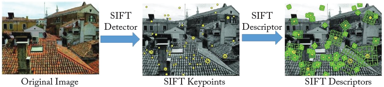
Figure 2.6: An example of the SIFT detector and descriptor: (left) an input image, (middle) some of the detected keypoints with their corresponding scales and orientations, and (right) SIFT descriptors–a 16 × 16 neighborhood around each keypoint is divided into 16 sub-blocks of 4 × 4 size.
2.2.3 SPEEDED-UP ROBUST FEATURES (SURF)
SURF [Bay et al., 2008] is a speeded up version of SIFT. In SIFT, the Laplacian of Gaussian is approximated with the DoG to construct a scale-space. SURF speeds up this process by approximating the LoG with a box filter. Thus, a convolution with a box filter can easily be computed with the help of integral images and can be performed in parallel for different scales.
Keypoint Localization
In the first step, a blob detector based on the Hessian matrix is used to localize keypoints. The determinant of the Hessian matrix is used to select both the location and scale of the potential keypoints. More precisely, for an image I with a given point p = (x, y), the Hessian matrix H(p, σ) at point p and scale σ, is defined as follows:

where Lxx (p, σ) is the convolution of the second-order derivative of the Gaussian, ![]() , with the image I at point p. However, instead of using Gaussian filters, SURF uses approximated Gaussian second-order derivatives, which can be evaluated using integral images at a very low computational cost. Thus, unlike SIFT, SURF does not require to iteratively apply the same filter to the output of a previously filtered layer, and scale-space analysis is done by keeping the same image and varying the filter size, i.e., 9 × 9, 25 × 15, 21 × 21, and 27 × 27.
, with the image I at point p. However, instead of using Gaussian filters, SURF uses approximated Gaussian second-order derivatives, which can be evaluated using integral images at a very low computational cost. Thus, unlike SIFT, SURF does not require to iteratively apply the same filter to the output of a previously filtered layer, and scale-space analysis is done by keeping the same image and varying the filter size, i.e., 9 × 9, 25 × 15, 21 × 21, and 27 × 27.
Then, a non-maximum suppression in a 3 × 3 × 3 neighborhood of each point in the image is applied to localize the keypoints in the image. The maxima of the determinant of the Hessian matrix are then interpolated in the scale and image space, using the method proposed by Brown and Lowe [2002].
Orientation Assignment
In order to achieve rotational invariance, the Haar wavelet responses in both the horizontal x and vertical y directions within a circular neighborhood of radius 6s around the keypoint are computed, where s is the scale at which the keypoint is detected. Then, the Haar wavelet responses in both the horizontal dx and vertical dy directions are weighted with a Gaussian centered at a keypoint, and represented as points in a 2D space. The dominant orientation of the keypoint is estimated by computing the sum of all the responses within a sliding orientation window of angle 60°. The horizontal and vertical responses within the window are then summed. The two summed responses is considered as a local vector. The longest orientation vector over all the windows determines the orientation of the keypoint. In order to achieve a balance between robustness and angular resolution, the size of the sliding window need to be chosen carefully.
Keypoint Descriptor
To describe the region around each keypoint p, a 20s × 20s square region around p is extracted and then oriented along the orientation of p. The normalized orientation region around p is split into smaller 4 × 4 square sub-regions. The Haar wavelet responses in both the horizontal dx and vertical dy directions are extracted at 5 × 5 regularly spaced sample points for each subregion. In order to achieve more robustness to deformations, noise and translation, The Haar wavelet responses are weighted with a Gaussian. Then, dx and dy are summed up over each subregion and the results form the first set of entries in the feature vector. The sum of the absolute values of the responses, |dx| and |dy|, are also computed and then added to the feature vector to encode information about the intensity changes. Since each sub-region has a 4D feature vector, concatenating all 4 × 4 sub-regions results in a 64D descriptor.
2.2.4 LIMITATIONS OF TRADITIONAL HAND-ENGINEERED FEATURES
Until recently, progress in computer vision was based on hand-engineering features. However, feature engineering is difficult, time-consuming, and requires expert knowledge on the problem domain. The other issue with hand-engineered features such as HOG, SIFT, SURF, or other algorithms like them, is that they are too sparse in terms of information that they are able to capture from an image. This is because the first-order image derivatives are not sufficient features for the purpose of most computer vision tasks such as image classification and object detection. Moreover, the choice of features often depends on the application. More precisely, these features do not facilitate learning from previous learnings/representations (transfer learning). In addition, the design of hand-engineered features is limited by the complexity that humans can put in it. All these issues are resolved using automatic feature learning algorithms such as deep neural networks, which will be addressed in the subsequent chapters (i.e., Chapters 3, 4, 5, and 6).
2.3 MACHINE LEARNING CLASSIFIERS
Machine learning is usually divided into three main areas, namely supervised, unsupervised, and semi-supervised. In the case of the supervised learning approach, the goal is to learn a mapping from inputs to outputs, given a labeled set of input-output pairs. The second type of machine learning is the unsupervised learning approach, where we are only given inputs, and the goal is to automatically find interesting patterns in the data. This problem is not a well-defined problem, because we are not told what kind of patterns to look for. Moreover, unlike supervised learning, where we can compare our label prediction for a given sample to the observed value, there is no obvious error metric to use. The third type of machine learning is semi-supervised learning, which typically combines a small amount of labeled data with a large amount of unlabeled data to generate an appropriate function or classifier. The cost of the labeling process of a large corpus of data is infeasible, whereas the acquisition of unlabeled data is relatively inexpensive. In such cases, the semi-supervised learning approach can be of great practical value.
Another important class of machine learning algorithms is “reinforcement learning,” where the algorithm allows agents to automatically determine the ideal behavior given an observation of the world. Every agent has some impact on the environment, and the environment provides reward feedback to guide the learning algorithm. However, in this book our focus is mainly on the supervised learning approach, which is the most widely used machine learning approach in practice.
A wide range of supervised classification techniques has been proposed in the literature. These methods can be divided into three different categories, namely linear (e.g., SVM [Cortes, 1995]; logistic regression; Linear Discriminant Analysis (LDA) [Fisher, 1936]), nonlinear (e.g., Multi Layer Perceptron (MLP), kernel SVM), and ensemble-based (e.g., RDF [Breiman, 2001, Quinlan, 1986]; AdaBoost [Freund and Schapire, 1997]) classifiers. The goal of ensemble methods is to combine the predictions of several base classifiers to improve generalization over a single classifier. The ensemble methods can be divided into two categories, namely averaging (e.g., Bagging methods; Random Decision Forests [Breiman, 2001, Quinlan, 1986]) and boosting (e.g., AdaBoost [Freund and Schapire, 1997]; Gradient Tree Boosting [Friedman, 2000]). In the case of the averaging methods, the aim is to build several classifiers independently and then to average their predictions. For the boosting methods, base “weak” classifiers are built sequentially and one tries to reduce the bias of the combined overall classifier. The motivation is to combine several weak models to produce a powerful ensemble.
Our definition of a machine learning classifier that is capable of improving computer vision tasks via experience is somewhat abstract. To make this more concrete, in the following we describe three widely used linear (SVM), nonlinear (kernel SVM) and ensemble (RDF) classifiers in some detail.
2.3.1 SUPPORT VECTOR MACHINE (SVM)
SVM [Cortes, 1995] is a supervised machine learning algorithm used for classification or regression problems. SVM works by finding a linear hyperplane which separates the training dataset into two classes. As there are many such linear hyperplanes, the SVM algorithm tries to find the optimal separating hyperplane (as shown in Fig. 2.7) which is intuitively achieved when the distance (also known as the margin) to the nearest training data samples is as large as possible. It is because, in general, the larger the margin the lower the generalization error of the model.
Mathematically, SVM is a maximum margin linear model. Given a training dataset of n samples of the form {(x1, y1), …, (xn, yn)}, where xi is an m-dimensional feature vector and yi = {1, – 1} is the class to which the sample xi belongs to. The goal of SVM is to find the maximum-margin hyperplane which divides the group of samples for which yi = 1 from the group of samples for which yi = –1. As shown in Fig. 2.7b (the bold blue line), this hyperplane can be written as the set of sample points satisfying the following equation:
where w is the normal vector to the hyperplane. More precisely, any samples above the hyperplane should have label 1, i.e., xi s.t. wTXi + b > 0 will have corresponding yi = 1. Similarly, any samples below the hyperplane should have label –1, i.e., WT xi s.t. wT xi + b < 0 will have corresponding yi, = –1.
Notice that there is some space between the hyperplane (or decision boundary, which is the bold blue line in Fig. 2.7b) and the nearest data samples of either class. Thus, the sample data is rescaled such that anything on or above the hyperplane wTXi + b + = 1 is of one class with label 1, and anything on or below the hyperplane wTXi + b = – 1 is of the other class with label – 1. Since these two new hyperplanes are parallel, the distance between them is ![]() , as shown in Fig. 2.7c.
, as shown in Fig. 2.7c.
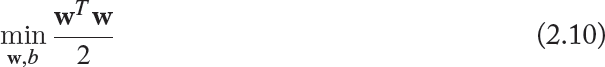
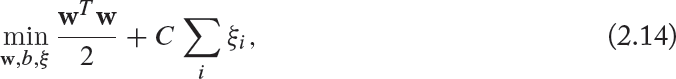
Recall that SVM tries to maximize the distance between these two new hyperplanes demarcating two classes, which is equivalent to minimizing ![]() . Thus, SVM is learned by solving the following primal optimization problem:
. Thus, SVM is learned by solving the following primal optimization problem:
subject to:
Soft-margin Extension
In the case where the training samples are not perfectly linearly separable, SVM can allow some samples of one class to appear on the other side of the hyperplane (boundary) by introducing slack variables, an ξi for each sample xi as follows:

subject to:
Unlike deep neural networks, which will be introduced in Chapter 3, linear SVMs can only solve problems that are linearly separable, i.e., where the data samples belonging to class 1 can be separated from the samples belonging to class 2 by a hyperplane as shown in Fig. 2.7. However, in many cases, the data samples are not linearly separable.
Nonlinear Decision Boundary
SVM can be extended to nonlinear classification by projecting the original input space (![]() ) into a high-dimensional space (
) into a high-dimensional space (![]() ), where a separating hyperplane can hopefully be found. Thus, the formulation of the quadratic programming problem is as above (Eq. (2.12) and Eq. (2.13)), but with all xi replaced with ϕ(xi), where ϕ provides a higher-dimensional mapping.
), where a separating hyperplane can hopefully be found. Thus, the formulation of the quadratic programming problem is as above (Eq. (2.12) and Eq. (2.13)), but with all xi replaced with ϕ(xi), where ϕ provides a higher-dimensional mapping.
subject to:


Figure 2.7: For two classes, separable training datasets, such as the one shown in (a), there are lots of possible linear separators as shown with the blue lines in (a). Intuitively, a separating hyperplane (also called decision boundary) drawn in the middle of the void between the data samples of the two classes (the bold blue line in (b)) seems better than the ones shown in (a). SVM defines the criterion for a decision boundary that is maximally far away from any data point. This distance from the decision surface to the closest data point determines the margin of the classifier as shown in (b). In the hard-margin SVM, (b), a single outlier can determine the decision boundary, which makes the classifier overly sensitive to the noise in the data. However, a soft margin SVM classifier, shown in (c), allows some samples of each class to appear on the other side of the decision boundary by introducing slack variables for each sample. (d) Shows an example where classes are not separable by a linear decision boundary. Thus, as shown in (e), the original input space ![]() is projected onto
is projected onto ![]() , where a linear decision boundary can be found, i.e., using the kernel trick.
, where a linear decision boundary can be found, i.e., using the kernel trick.
In the case that D ≫ d, there are many more parameters to learn for w. In order to avoid that, the dual form of SVM is used for optimization problem.

subject to:

where C is a hyper-parameter which controls the degree of misclassification of the model, in case classes are not linearly separable.
Kernel Trick
Since ϕ(xi) is in a high-dimensional space (even infinite-dimensional space), calculating ϕ(xi)T · ϕ(xj) maybe intractable. However, there are special kernel functions, such as linear, polynomial, Gaussian, and Radial Basis Function (RBF), which operate on the lower dimension vectors xi and xj to produce a value equivalent to the dot-product of the higher-dimensional vectors. For example, consider the function ![]() , where
, where

It is interesting to note that for the given function ϕ in Eq. (2.18),
2. FEATURES AND CLASSIFIERS
Thus, instead of calculating ϕ(xi)T · ϕ(xj), the polynomial kernel function K(xi, xj) = (1 + xiT xj)2 is calculated to produce a value equivalent to the dot-product of the higher-dimensional vectors, ϕ(xi)T · ϕ(xj).
Note that the dual optimization problem is exactly the same, except that the dot product ϕ(xi)T · ϕ(xj) is replaced by a kernel K(xi, xj) which corresponds to the dot product of ϕ(xi) and ϕ(xj) in the new space.
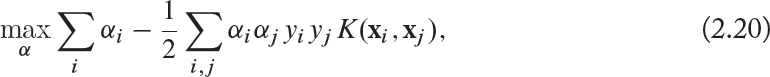
subject to:

In summary, linear SVMs can be thought of as a single layer classifier and kernel SVMs can be thought of as a 2 layer neural network. However, unlike SVMs, Chapter 3 shows that deep neural networks are typically built by concatenating several nonlinear hidden layers, and thus, can extract more complex pattern from data samples.
A random decision forest [Breiman, 2001, Quinlan, 1986] is an ensemble of decision trees. As shown in Fig. 2.8a, each tree consists of split and leaf nodes. A split node performs binary classification based on the value of a particular feature of the features vector. If the value of the particular feature is less than a threshold, then the sample is assigned to the left partition, else to the right partition. Figure 2.8b shows an illustrative decision tree used to figure out whether a photo represents and indoor or an outdoor scene. If the classes are linearly separable, after log2(c) decisions each sample class will get separated from the remaining c – 1 classes and reach a leaf node. For a given feature vector f, each tree predicts independently its label and a majority voting scheme is used to predict the final label of the feature vector. It has been shown that random decision forests are fast and effective multi-class classifiers [Shotton et al., 2011].
Training
Each tree is trained on a randomly selected samples of the training data (usually ![]() samples of the training data). The remaining samples of the training data are used for validation. A subset of features is randomly selected for each split node. Then, we search for the best feature f[i] and an associated threshold τi that maximize the information gain of the training data after partitioning. Let H(Q) be the original entropy of the training data and H(Q |{f[i], τi}) the entropy of Q after partitioning it into “left” and “right” partitions, Ql; and Qr. The information gain, G, is given by
samples of the training data). The remaining samples of the training data are used for validation. A subset of features is randomly selected for each split node. Then, we search for the best feature f[i] and an associated threshold τi that maximize the information gain of the training data after partitioning. Let H(Q) be the original entropy of the training data and H(Q |{f[i], τi}) the entropy of Q after partitioning it into “left” and “right” partitions, Ql; and Qr. The information gain, G, is given by

Figure 2.8: (a) A decision tree is a set of nodes and edges organized in a hierarchical fashion. The split (or internal) nodes are denoted with circles and the leaf (or terminal) nodes with squares. (b) A decision tree is a tree where each split node stores a test function which is applied to the input data. Each leaf stores the final label (here whether “indoor” or “outdoor”).
where

and |Ql| and |Qr| denote the number of data samples in the left and right partitions. The entropy of Ql is given by

where pi is the number of samples of class i in Ql divided by Ql. The feature and the associated threshold which maximize the gain are selected as the splitting test for that node
Entropy and Information Gain: The entropy and information gain are two important concepts in the RDF training process. These concepts are usually discussed in information theory or probability courses and are briefly discussed below.
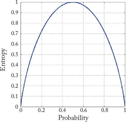
Information entropy is defined as a measure of the randomness in the information being processed. More precisely, the higher the entropy, the lower the information content. Mathematically, given a discrete random variable X with possible values {x1 …, xn} and a probability mass function P(X), the entropy H (also called Shannon entropy) can be written as follows:

For example, an action such as flipping a coin that has no affinity for “head” or “tail,” provides information that is random (X with possible values of {“head,” “tail”}). Therefore, Eq. (2.26) can be written as follows:
As shown in Fig. 2.9, this binary entropy function (Eq. (2.27)) reaches its maximum value (uncertainty is at a maximum) when the probability is ![]() , meaning that P(X = “head”) =
, meaning that P(X = “head”) = ![]() or similarly P(X = “tail”) = 2
or similarly P(X = “tail”) = 2![]() . The entropy function reaches its minimum value (i.e., zero) when probability is 1 or 0 with complete certainty P(X = “head” = 1) or P(X = “head” = 0) respectively.
. The entropy function reaches its minimum value (i.e., zero) when probability is 1 or 0 with complete certainty P(X = “head” = 1) or P(X = “head” = 0) respectively.
Information gain is defined as the change in information entropy H from a prior state to a state that takes some information (t) and can be written as follows:
If a partition consists of only a single class, it is considered as a leaf node. Partitions consisting of multiple classes are further partitioned until either they contain single classes or the tree reaches its maximum height. If the maximum height of the tree is reached and some of its leaf nodes contain labels from multiple classes, the empirical distribution over the classes associated with the subset of the training samples v, which have reached that leaf, is used as its label. Thus, the probabilistic leaf predictor model for the t-th tree is pt (c|v), where c ∈ {ck} denotes the class.
Classification
Once a set of decision trees have been trained, given a previously unseen sample xj, each decision tree hierarchically applies a number of predefined tests. Starting at the root, each split node applies its associated split function to xj. Depending on the result of the binary test the data is sent to the right or the left child. This process is repeated until the data point reaches a leaf node. Usually the leaf nodes contain a predictor (e.g., a classifier) which associates an output (e.g., a class label) to the input xj. In the case of forests, many tree predictors are combined together to form a single forest prediction:
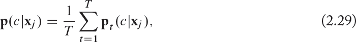
where T denotes the number of decision trees in the forest.
Traditional computer vision systems consist of two steps: feature design and learning algorithm design, both of which are largely independent. Thus, computer vision problems have traditionally been approached by designing hand-engineered features such as HOG [Triggs and Dalal, 2005], SIFT [Lowe, 2004], and SURF [Bay et al., 2008] that lack in generalizing well to other domains, are time consuming, expensive, and require expert knowledge on the problem domain. These feature engineering processes are usually followed by learning algorithms such as SVM [Cortes, 1995] and RDF [Breiman, 2001, Quinlan, 1986]. However, progress in deep learning algorithms resolves all these issues, by training a deep neural network for feature extraction and classification in an end-to-end learning framework. More precisely, unlike traditional approaches, deep neural networks learn to simultaneously extract features and classify data samples. Chapter 3 will discuss deep neural networks in detail.

Figure 2.10: RDF classification for a test sample xj. During testing the same test sample is passed through each decision tree. At each internal node a test is applied and the test sample is sent to the appropriate child. This process is repeated until a leaf is reached. At the leaf the stored posterior pt (c|xj) is read. The forest class posterior p(c|xj) is the average of all decision tree posteriors.