CNN Learning
In Chapter 4, we discussed different architecture blocks of the CNN and their operational details. Most of these CNN layers involve parameters which are required to be tuned appropriately for a given computer vision task (e.g., image classification and object detection). In this chapter, we will discuss various mechanisms and techniques that are used to set the weights in deep neural networks. We will first cover concepts such as weight initialization and network regularization in Sections 5.1 and 5.2, respectively, which helps in a successful optimization of the CNNs. Afterward, we will introduce gradient-based parameter learning for CNNs in Section 5.3, which is quite similar to the MLP parameter learning process discussed in Chapter 3. The details of neural network optimization algorithms (also called “solvers”) will come in Section 5.4. Finally in Section 5.5, we will explain various types of approaches which are used for the calculation of the gradient during the error back-propagation process.
A correct weight initialization is the key to stably train very deep networks. An ill-suited initialization can lead to the vanishing or exploding gradient problem during error back-propagation. In this section, we introduce several approaches to perform weight initialization and provide comparisons between them to illustrate their benefits and problems. Note that the discussion below pertains to the initialization of neuron weights within a network and the biases are usually set to zero at the start of the network training. If all the weights are also set to zero at the start of training, the weight updates will be identical (due to symmetric outputs) and the network will not learn anything useful. To break this symmetry between neural units, the weights are initialized randomly at the start of the training. In the following, we describe several popular approaches to network initialization.
5.1.1 GAUSSIAN RANDOM INITIALIZATION
A common approach to weight initialization in CNNs is the Gaussian random initialization technique. This approach initializes the convolutional and the fully connected layers using random matrices whose elements are sampled from a Gaussian distribution with zero mean and a small standard deviation (e.g., 0.1 and 0.01).
5.1.2 UNIFORM RANDOM INITIALIZATION
The uniform random initialization approach initializes the convolutional and the fully connected layers using random matrices whose elements are sampled from a uniform distribution (instead of a normal distribution as in the earlier case) with a zero mean and a small standard deviation (e.g., 0.1 and 0.01). The uniform and normal random initializations generally perform identically. However, the training of very deep networks becomes a problem with a random initialization of weights from a uniform or normal distribution [Simonyan and Zisserman, 2014b]. The reason is that the forward and backward propagated activations can either diminish or explode when the network is very deep (see Section 3.2.2).
5.1.3 ORTHOGONAL RANDOM INITIALIZATION
Orthogonal random initialization has also been shown to perform well in deep neural networks [Saxe et al., 2013]. Note that the Gaussian random initialization is only approximately orthogonal. For the orthogonal random initialization, a random weight matrix is decomposed by applying e.g., an SVD. The orthogonal matrix (U) is then used for the weight initialization of the CNN layers.
5.1.4 UNSUPERVISED PRE-TRAINING
One approach to avoid the gradient diminishing or exploding problem is to use layer-wise pretraining in an unsupervised fashion. However, this type of pre-training has found more success in the training of deep generative networks, e.g., Deep Belief Networks [Hinton et al., 2006] and Auto-encoders [Bengio et al., 2007]. The unsupervised pre-training can be followed by a supervised fine-tuning stage to make use of any available annotations. However, due to the new hyper-parameters, the considerable amount of effort involved in such an approach and the availability of better initialization techniques, layer-wise pre-training is seldom used now to enable the training of CNN-based very deep networks. We describe some of the more successful approaches to initialize deep CNNs next.
A random initialization of a neuron makes the variance of its output directly proportional to the number of its incoming connections (a neuron’s fan-in measure). To alleviate this problem, Glorot and Bengio [2010] proposed to randomly initialize the weights with a variance measure that is dependent on the number of incoming and outgoing connections (![]() and
and ![]() respectively) from a neuron,
respectively) from a neuron,

where w are network weights. Note that the fan-out measure is used in the variance above to balance the back-propagated signal as well. Xavier initialization works quite well in practice and leads to better convergence rates. But a number of simplistic assumptions are involved in the above initialization, among which the most prominent is that a linear relationship between the input and output of a neuron is assumed. In practice all the neurons contain a nonlinearity term which makes Xavier initialization statistically less accurate.
5.1.6 RELU AWARE SCALED INITIALIZATION
He et al. [2015a] suggested an improved version of the scaled (or Xavier) initialization noting that the neurons with a ReLU nonlinearity do not follow the assumptions made for the Xavier initialization. Precisely, since the ReLU activation reduces nearly half of the inputs to zero, therefore the variance of the distribution from which the initial weights are randomly sampled should be

The ReLU aware scaled initialization works better compared to Xavier initialization for recent architectures which are based on the ReLU nonlinearity.
5.1.7 LAYER-SEQUENTIAL UNIT VARIANCE
The layer-sequential unit variance (LSUV) initialization is a simple extension of the orthonormal weight initialization in deep network layers [Mishkin and Matas, 2015]. It combines the benefits of batch-normalization and the orthonormal weight initialization to achieve an efficient training for very deep networks. It proceeds in two steps, described below.
• Orthogonal initialization—In the first step, all the weight layers (convolutional and fully connected) are initialized with orthogonal matrices.
• Variance normalization—In the second step, the method starts from the initial toward the final layers in a sequential manner and the variance of each layer output is normalized to one (unit variance). This is similar to the batch normalization layer, which normalizes the output activations for each batch to be zero centered with a unit variance. However, different from batch normalization which is applied during the training of the network, LSUV is applied while initializing the network and therefore saves the overhead of normalization for each batch during the training iterations.
In practical scenarios, it is desirable to train very deep networks, but we do not have a large amount of annotated data available for many problem settings. A very successful practice in such cases is to first train the neural network on a related but different problem, where a large amount of training data is already available. Afterward, the learned model can be “adapted” to the new task by initializing with weights pre-trained on the larger dataset. This process is called “fine-tuning” and is a simple, yet effective, way to transfer learning from one task to another (sometimes interchangeably referred to as domain transfer or domain adaptation). As an example, in order to perform scene classification on a relatively small dataset, MIT-67, the network can be initialized with the weights learned for object classification on a much larger dataset such as ImageNet [Khan et al., 2016b].
Transfer Learning is an approach to adapt and apply the knowledge acquired on another related task to the task at hand. Depending on our CNN architecture, this approach can take two forms.
• Using a Pre-trained Model: If one wants to use an off-the-shelf CNN architecture (e.g., AlexNet, GoogleNet, ResNet, DenseNet) for a given task, an ideal choice is to adopt the available pre-trained models that are learned on huge datasets such as ImageNet (with 1.2 million images)a and Places205 (with 2.5 million images).b
The pre-trained model can be tailored for a given task, e.g., by changing the dimensions of output neurons (to cater for a different number of classes), modifying the loss function and learning the final few layers from scratch (normally learning the final 2-3 layers suffices for most cases). If the dataset available for the end-task is sufficiently large, the complete model can also be fine-tuned on the new dataset. For this purpose, small learning rates are used for the initial pre-trained CNN layers, so that the learning previously acquired on the large-scale dataset (e.g., ImageNet) is not completely lost. This is essential, since it has been shown that the features learned over large-scale datasets are generic in nature and can be used for new tasks in computer vision [Azizpour et al., 2016, Sharif Razavian et al., 2014].
• Using a Custom Architecture: If one opts for a customized CNN architecture, transfer learning can still be helpful if the target dataset is constrained in terms of size and diversity. To this end, one can first train the custom architecture on a large scale annotated dataset and then use the resulting model in the same manner as described in the bullet point above.
Alongside the simple fine-tuning approach, more involved transfer learning approaches have also been proposed in the recent literature, e.g., Anderson et al. [2016] learns the way pre-trained model parameters are shifted on new datasets. The learned transformation is then applied to the network parameters and the resulting activations beside the pre-trained (non-tunable) network activations are used in the final model.
aPopular deep learning libraries host a wide variety of pre-trained CNN models, e.g.,
Tensorflow (https://github.com/tensorflow/models),
Torch (https://github.com/torch/torch7/wiki/ModelZoo),
Keras (https://github.com/albertomontesg/keras-model-zoo,
Caffe (https://github.com/BVLC/caffe/wiki/Model-Zoo),
MatConvNet (http://www.vlfeat.org/matconvnet/pretrained/).
Since deep neural networks have a large number of parameters, they tend to over-fit on the training data during the learning process. By over-fitting, we mean that the model performs really well on the training data but it fails to generalize well to unseen data. It, therefore, results in an inferior performance on new data (usually the test set). Regularization approaches aim to avoid this problem using several intuitive ideas which we discuss below. We can categorize common regularization approaches into the following classes, based on their central idea:
• approaches which regularize the network using data level techniques (e.g., data augmentation);
• approaches which introduce stochastic behavior in the neural activations (e.g., dropout and drop connect);
• approaches which normalize batch statistics in the feature activations (e.g., batch normalization);
• approaches which use decision level fusion to avoid over-fitting (e.g., ensemble model averaging);
• approaches which introduce constraints on the network weights (e.g., ℓ1 norm, ℓ2 norm, max-norm, and elastic net constraints); and
• approaches which use guidance from a validation set to halt the learning process (e.g., early stopping).
Next, we discuss the above-mentioned approaches in detail.
Data augmentation is the easiest, and often a very effective way of enhancing the generalization power of CNN models. Especially for cases where the number of training examples is relatively low, data augmentation can enlarge the dataset (by factors of 16×, 32×, 64×, or even more) to allow a more robust training of large-scale models.
Data augmentation is performed by making several copies from a single image using straightforward operations such as rotations, cropping, flipping, scaling, translations, and shearing (see Fig. 5.1). These operations can be performed separately or combined together to form copies, which are both flipped and cropped.
Color jittering is another common way of performing data augmentation. A simple form of this operation is to perform random contrast jittering in an image. One could also find the principal color directions in the R, G, and B channels (using PCA) and then apply a random offset along these directions to change the color values of the whole image. This effectively introduces color and illumination invariance in the learned model [Krizhevsky et al., 2012].
Another approach for data augmentation is to utilize synthetic data, alongside the real data, to improve the generalization ability of the network [Rahmani and Mian, 2016, Rahmani et al., 2017, Shrivastava et al., 2016]. Since synthetic data is usually available in large quantities from rendering engines, it effectively extends the training data, which helps avoid over-fitting.
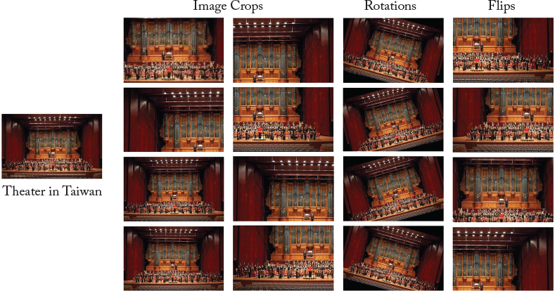
Figure 5.1: The figure shows an example of data augmentation using crops (column 1 and 2), rotations (column 3) and flips (column 4). Since the input image is quite complex (has several objects), data augmentation allows the network to figure out some possible variations of the same image, which still denote the same scene category, i.e., a theater.
One of the most popular approaches for neural network regularization is the dropout technique [Srivastava et al., 2014]. During network training, each neuron is activated with a fixed probability (usually 0.5 or set using a validation set). This random sampling of a sub-network within the full-scale network introduces an ensemble effect during the testing phase, where the full network is used to perform prediction. Activation dropout works really well for regularization purposes and gives a significant boost in performance on unseen data in the test phase.
Let us consider a CNN that is composed of L weight layers, indexed by l ∈ {1 … L}. Since dropout has predominantly been applied to Fully Connected (FC) layers in the literature, we consider the simpler case of FC layers here. Given output activations al–1 from the previous layer, a FC layer performs an affine transformation followed by a element-wise nonlinearity, as follows:
Here, at–1 ∈ ℝm and b ∈ ℝm denote the activations and biases respectively. The input and output dimensions of the FC layer are denoted by n and m respectively. W ∈ ℝm×n is the weight matrix and f(·) is the ReLU activation function.
The random dropout layer generates a mask m ∈ ?m, where each element mi is independently sampled from a Bernoulli distribution with a probability “p” of being “on,” i.e., a neuron fires:
This mask is used to modify the output activations al:
where, “o” denotes the Hadamard product. The Hadamard product denotes a simple element wise matrix multiplication between the mask and the CNN activations.
Another similar approach to dropout is the drop-connect [Wan et al., 2013], which randomly deactivates the network weights (or connections between neurons) instead of randomly reducing the neuron activations to zero.
Similar to dropout, drop-connect performs a masking out operation on the weight matrix instead of the output activations, therefore:
where “o” denotes the Hadamard product as in the case of dropout.
Batch normalization [Ioffe and Szegedy, 2015] normalizes the mean and variance of the output activations from a CNN layer to follow a unit Gaussian distribution. It proves to be very useful for the efficient training of a deep network because it reduces the “internal covariance shift” of the layer activations. Internal covariance shift refers to the change in the distribution of activations of each layer as the parameters are updated during training. If the distribution, which a hidden layer of a CNN is trying to model, keeps on changing (i.e., the internal covariance shift is high), the training process will slow down and the network will take a long time to converge (simply because it is hard to reach a static target than to reach a continuously shifting target). The normalization of this distribution leads us to a consistent activation distribution during the training process, which enhances the convergence and avoids network instability issues such as the vanishing/exploding gradients and activation saturation.
Reflecting on what we have already studied in Chapter 4, this normalization step is similar to the whitening transform (applied as an input pre-processing step) which enforces the inputs to follow a unit Gaussian distribution with zero mean and unit variance. However, different to the whitening transform, batch normalization is applied to the intermediate CNN activations and can be integrated in an end-to-end network because of its differentiable computations.
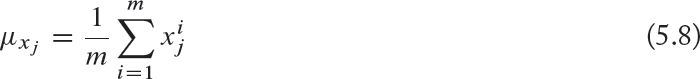
The batch normalization operation can be implemented as a layer in a CNN. Given a set of activations ![]() (where
(where ![]() has n dimensions) from a CNN layer corresponding to a specific input batch with m images, we can compute the first and second order statistics (mean and variance respectively) of the batch for each dimension of activations as follows:
has n dimensions) from a CNN layer corresponding to a specific input batch with m images, we can compute the first and second order statistics (mean and variance respectively) of the batch for each dimension of activations as follows:

where ![]() and
and ![]() . represent the mean and variance for the jth activation dimension computed over a batch, respectively. The normalized activation operation is represented as:
. represent the mean and variance for the jth activation dimension computed over a batch, respectively. The normalized activation operation is represented as:

Just the normalization of the activations is not sufficient, because it can alter the activations and disrupt the useful patterns that are learned by the network. Therefore, the normalized activations are rescaled and shifted to allow them to learn useful discriminative representations:
where γj and ßj are the learnable parameters which are tuned during error back-propagation.
Note that batch normalization is usually applied after the CNN weight layers, before applying the nonlinear activation function. Batch normalization is an important tool that is used in state of the art CNN architectures (examples in Chapter 6). We briefly summarize the benefits of using batch normalization below.
• In practice, the network training becomes less sensitive to hyper-parameter choices (e.g., learning rate) when batch normalization is used [Ioffe and Szegedy, 2015].
• It stabilizes the training of very deep networks and provides robustness against bad weight initializations. It also avoids the vanishing gradient problem and the saturation of activation functions (e.g., tanh and sigmoid).
• Batch normalization greatly improves the network convergence rate. This is very important because very deep network architectures can take several days (even with reasonable hardware resources) to train on large-scale datasets.
• It integrates the normalization in the network by allowing back-propagation of errors through the normalization layer, and therefore allows end-to-end training of deep networks.
• It makes the model less dependent on regularization techniques such as dropout. Therefore, recent architectures do not use dropout when batch normalization is extensively used as a regularization mechanism [He et al., 2016a].
5.2.5 ENSEMBLE MODEL AVERAGING
The ensemble averaging approach is another simple, but effective, technique where a number of models are learned instead of just a single model. Each model has different parameters due to different random initializations, different hyper-parameter choices (e.g., architecture, learning rate) and/or different sets of training inputs. The output from these multiple models is then combined to generate a final prediction score. The prediction combination approach can be a simple output averaging, a majority voting scheme or a weighted combination of all predictions. The final prediction is more accurate and less prone to over-fitting compared to each individual model in the ensemble. The committee of experts (ensemble) acts as an effective regularization mechanism which enhances the generalization power of the overall system.
The ℓ2 regularization penalizes large values of the parameters w during the network training. This is achieved by adding a term with ℓ2 norm of the parameter values weighted by a hyper-parameter λ, which decides on the strength of penalization (in practice half of the squared magnitude times λ is added to the error function to ensure a simpler derivative term). Effectively, this regularization encourages small and spread-out weight distributions over large values concentrated over only few neurons. Consider a simple network with only a single hidden layer with parameters w and output pn, n ∈ [1, N] when the output layer has N neurons. If the desired output is denoted by yn, we can use an euclidean objective function with ℓ2 regularization to update the parameters as follows:
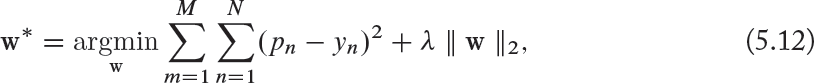
where M denote the number of training examples. Note that, as we will discuss later, ℓ2 regularization performs the same operation as the weight decay technique. This approach is called “weight decay” because applying ℓ2 regularization means that the weights are updated linearly (since the derivative of the regularizer term is λw for each neuron).
The ℓ1 regularization technique is very similar to the ℓ2 regularization, with the only difference being that the regularizer term uses the ℓ1 norm of weights instead of an ℓ2 norm. A hyper-parameter λ is used to define the strength of regularization. For a single layered network with parameters w, we can denote the parameter optimization process using l1 norm as follows:
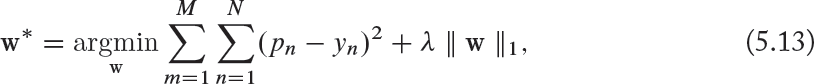
where N and M denote the number of output neurons and the number of training examples respectively. This effectively leads to sparse weight vectors for each neuron with most of the incoming connections having very small weights.
5.2.8 ELASTIC NET REGULARIZATION
Elastic net regularization linearly combines both ℓ1 and ℓ2 regularization techniques by adding a term ![]() for each weight value. This results in sparse weights and often performs better than the individual ℓ1 and ℓ2 regularizations, each of which is a special case of elastic net regularization. For a single-layered network with parameters w, we can denote the parameter optimization process as follows:
for each weight value. This results in sparse weights and often performs better than the individual ℓ1 and ℓ2 regularizations, each of which is a special case of elastic net regularization. For a single-layered network with parameters w, we can denote the parameter optimization process as follows:

where N and M denote the number of output neurons and the number of training examples, respectively.
The max-norm constraint is a form of regularization which puts an upper bound on the norm of the incoming weights of each neuron in a neural network layer. As a result, the weight vector w must follow the constraint || w ||2< h, where h is a hyper-parameter, whose value is usually set based on the performance of the network on a validation set. The benefit of using such a regularization is that the network parameters are guaranteed to remain in a reasonable numerical range even when high values of learning rates are used during network training. In practice, this leads to a better stability and performance [Srivastava et al., 2014].
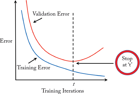
The over-fitting problem occurs when a model performs very well on the training set but behaves poorly on unseen data. Early stopping is applied to avoid overfitting in the iterative gradient-based algorithms. This is achieved by evaluating the performance on a held-out validation set at different iterations during the training process. The training algorithm can continue to improve on the training set until the performance on the validation set also improves. Once there is a drop in the generalization ability of the learned model, the learning process can be stopped or slowed down (Fig. 5.2).
Having discussed the concepts which enable successful training of deep neural networks (e.g., correct weight initialization and regularization techniques), we dive into the details of the network learning process. Gradient-based algorithms are the most important tool to optimally train such networks on large-scale datasets. In the following, we discuss different variants of optimizers for CNNs.
5.3 GRADIENT-BASED CNN LEARNING
The CNN learning process tunes the parameters of the network such that the input space is correctly mapped to the output space. As discussed before, at each training step, the current estimate of the output variables is matched with the desired output (often termed the “ground-truth” or the “label space”). This matching function serves as an objective function during the CNN training and it is usually called the loss function or the error function. In other words, we can say that the CNN training process involves the optimization of its parameters such that the loss function is minimized. The CNN parameters are the free/tunable weights in each of its layers (e.g., filter weights and biases of the convolution layers) (Chapter 4).
An intuitive, but simple, way to approach this optimization problem is by repeatedly updating the parameters such that the loss function progressively reduces to a minimum value. It is important to note here that the optimization of nonlinear models (such as CNNs) is a hard task, exacerbated by the fact that these models are mostly composed of a large number of tunable parameters. Therefore, instead of solving for a globally optimal solution, we iteratively search for the locally optimal solution at each step. Here, the gradient-based methods come as a natural choice, since we need to update the parameters in the direction of the steepest descent. The amount of parameter update, or the size of the update step is called the “learning rate.” Each iteration which updates the parameters using the complete training set is called a “training epoch.” We can write each training iteration at time t using the following parameter update equation:
where F(·) denotes the function represented by the neural network with parameters θ, ∇ represents the gradient, and η denotes the learning rate.
As we discussed in the previous section, gradient descent algorithms work by computing the gradient of the objective function with respect to the neural network parameters, followed by a parameter update in the direction of the steepest descent. The basic version of the gradient descent, termed “batch gradient descent,” computes this gradient on the entire training set. It is guaranteed to converge to the global minimum for the case of convex problems. For non-convex problems, it can still attain a local minimum. However, the training sets can be very large in computer vision problems, and therefore learning via the batch gradient descent can be prohibitively slow because for each parameter update, it needs to compute the gradient on the complete training set. This leads us to the stochastic gradient descent, which effectively circumvents this problem.
5.3.2 STOCHASTIC GRADIENT DESCENT
Stochastic Gradient Descent (SGD) performs a parameter update for each set of input and output that are present in the training set. As a result, it converges much faster compared to the batch gradient descent. Furthermore, it is able to learn in an “online manner” where the parameters can be tuned in the presence of new training examples. The only problem is that its convergence behavior is usually unstable, especially for relatively larger learning rates and when the training datasets contain diverse examples. When the learning rate is appropriately set, the SGD generally achieves a similar convergence behavior, compared to the batch gradient descent, for both the convex and non-convex problems.
5.3.3 MINI-BATCH GRADIENT DESCENT
Finally, the mini-batch gradient descent method is an improved form of the stochastic gradient descent approach, which provides a decent trade-off between convergence efficiency and convergence stability by dividing the training set into a number of mini-batches, each consisting of a relatively small number of training examples. The parameter update is then performed after computing the gradients on each mini-batch. Note that the training examples are usually randomly shuffled to improve homogeneity of the training set. This ensures a better convergence rate compared to the Batch Gradient Descent and a better stability compared to the Stochastic Gradient Descent [Ruder, 2016].
After a general overview of the gradient descent algorithms in Section 5.3, we can note that there are certain caveats which must be avoided during the network learning process. As an example, setting the learning rate can be a tricky endeavor in many practical problems. The training process is often highly affected by the parameter initialization. Furthermore, the vanishing and exploding gradients problems can occur especially for the case of deep networks. The training process is also susceptible to get trapped into a local minima, saddle points or a high error plateau where the gradient is approximately zero in every direction [Pascanu et al., 2014]. Note that the saddle points (also called the “minmax points”) are those stationary points on the surface of the function, where the partial derivative with respect to its dimensions becomes zero (Fig. 5.3). In the following discussion we outline different methods to address these limitations of the gradient descent algorithms. Since our goal is to optimize over high-dimensional parameter spaces, we will restrict our discussion to the more feasible first-order methods and will not deal with the high-order methods (Newton’s method) which are ill-suited for large datasets.
Momentum-based optimization provides an improved version of SGD with better convergence properties. For example, the SGD can oscillate close to a local minima, resulting in an unnecessarily delayed convergence. The momentum adds the gradient calculated at the previous time-step (at–1) weighted by a parameter γ to the weight update equation as follows:

Figure 5.3: A saddle point shown as a red dot on a 3D surface. Note that the gradient is effectively zero, but it corresponds to neither a “minima” nor a “maxima” of the function.
where F(·) denotes the function represented by the neural network with parameters θ, ∇ represents the gradient and η denotes the learning rate.
The momentum term has physical meanings. The dimensions whose gradients point in the same direction are magnified quickly, while those dimensions whose gradients keep on changing directions are suppressed. Essentially, the convergence speed is increased because unnecessary oscillations are avoided. This can be understood as adding more momentum to the ball so that it moves along the direction of the maximum slope. Typically, the momentum is set to 0.9 during the SGD-based learning.
The momentum term introduced in the previous section would carry the ball beyond the minimum point. Ideally, we would like the ball to slow down when the ball reaches the minimum point and the slope starts ascending. This is achieved by the Nesterov momentum [Nesterov, 1983] which computes the gradient at the next approximate point during the parameter update process, instead of the current point. This gives the algorithm the ability to “look ahead” at each iteration and plan a jump such that the learning process avoids uphill steps. The update process can be represented as:

Figure 5.4: Comparison of the convergence behavior of the SGD with (right) and without (left) momentum.
where F(·) denotes the function represented by the neural network with parameters θ, ∇ represents the gradient operation, η denotes the learning rate and γ is the momentum.

Figure 5.5: Comparison of the convergence behavior of the SGD with momentum (left) and the Nesterov update (right). While momentum update can carry the solver quickly toward a local optima, it can overshoot and miss the optimum point. A solver with Nesterov update corrects its update by looking ahead and correcting for the next gradient value.
The momentum in the SGD refines the update direction along the slope of the error function. However, all parameters are updated at the same rate. In several cases, it is more useful to update each parameter differently, depending on its frequency in the training set or its significance for our end problem.
Adaptive Gradient (AdaGrad) algorithm [Duchi et al., 2011] provides a solution to this problem by using an adaptive learning rate for each individual parameter i. This is done at each time step t by dividing the learning rate of each parameter with the accumulation of the square of all the historical gradients for each parameter θi. This can be shown as follows:

where ![]() is the gradient at time-step t with respect to the parameter θi and ϵ is a very small term in the denominator to avoid division by zero. The adaptation of the learning rate for each parameter removes the need to manually set the value of the learning rate. Typically, η is kept fixed to a single value (e.g., 10–2 or 10–3) during the training phase. Note that AdaGrad works very well for sparse gradients, for which a reliable estimate of the past gradients is obtained by accumulating all of the previous time steps.
is the gradient at time-step t with respect to the parameter θi and ϵ is a very small term in the denominator to avoid division by zero. The adaptation of the learning rate for each parameter removes the need to manually set the value of the learning rate. Typically, η is kept fixed to a single value (e.g., 10–2 or 10–3) during the training phase. Note that AdaGrad works very well for sparse gradients, for which a reliable estimate of the past gradients is obtained by accumulating all of the previous time steps.
Although AdaGrad eliminates the need to manually set the value of the learning rate at different epochs, it suffers from the vanishing learning rate problem. Specifically, as the number of iterations grows (t is large), the sum of the squared gradients becomes large, making the effective learning rate very small. As a result, the parameters do not change in the subsequent training iterations. Lastly, it also needs an initial learning rate to be set during the training phase.
The Adaptive Delta (AdaDelta) algorithm [Zeiler, 2012] solves both these problems by accumulating only the last k gradients in the denominator term of Eq. (5.21). Therefore, the new update step can be represented as follows:

This requires the storage of the last k gradients at each iteration. In practice, it is much easier to work with a running average E[δ2]t, which can be defined as:
Here, γ has a similar function to the momentum parameter. Note that the above function implements an exponentially decaying average of the squared gradients for each parameter. The new update step is:


Note that we still did not get rid of the initial learning rate η. Zeiler [2012] noted that this can be avoided by making the units of the update step consistent by introducing a Hessian approximation in the update rule. This boils down to the following:
Note that we have considered here the local curvature of the function F to be approximately flat and replaced E[(Δθ)2]t (not known) with E[(Δθ)2]t–2 (known).
RMSprop [Tieleman and Hinton, 2012] is closely related to the AdaDelta approach, aiming to resolve the vanishing learning rate problem of AdaGrad. Similar to AdaDelta, it also calculates the running average as follows:
Here, a typical value of γ is 0.9. The update rule of the tunable parameters takes the following form:

5.4.6 ADAPTIVE MOMENT ESTIMATION
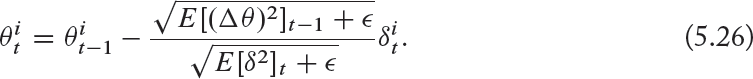
We stated that the AdaGrad solver suffers from the vanishing learning rate problem, but AdaGrad is very useful for cases where gradients are sparse. On the other hand, RMSprop does not reduce the learning rate to a very small value at higher time steps. However on the negative side, it does not provide an optimal solution for the case of sparse gradients. The ADAptive Moment Estimation (ADAM) [Kingma and Ba, 2014] approach estimates a separate learning rate for each parameter and combines the positives of both AdaGrad and RMSprop. The main difference between Adam and its two predecessors (RMSprop and AdaDelta) is that the updates are estimated by using both the first moment and the second moment of the gradient (as in Eqs. (5.26) and (5.28)). Therefore, a running average of gradients (mean) is maintained along with a running average of the squared gradients (variance) as follows:
where γ1 and γ2 are the parameters for running averages of the mean and the variance respectively. Since the initial moment estimates are set to zero, they can remain very small even after many iterations, especially when γ1,2 ≠ 1. To overcome this issue, the initialization bias-corrected estimates of E[δ]t and E[δ2]t are obtained as follows:


Figure 5.6: Convergence performance on the MNIST dataset using different neural network optimizers [Kingma and Ba, 2014]. (Figure used with permission.)
Very similar to what we studied in the case of AdaGrad, AdaDelta and RMSprop, the update rule for Adam is given by:

The authors found γ1 = 0.9, γ2 = 0.999, η = 0.001 to be good default values of the decay (γ) and learning (η) rates during the training process.
Figure 5.6 [Kingma and Ba, 2014] illustrates the convergence performance of the discussed solvers on the MNIST dataset for handwritten digit classification. Note that the SGD with Nesterov shows a good convergence behavior, however it requires a manual tuning of the learning rate hyper-parameter. Among the solvers with an adaptive learning rate, Adam performs the best in this example (also beating the manually tuned SGD-Nesterov solver). In practice, Adam usually scales very well to large-scale problems and exhibits nice convergence properties. That is why Adam is often a default choice for many computer vision applications based on deep learning.
5.5 GRADIENT COMPUTATION IN CNNS
We have discussed a number of layers and architectures for CNNs. In Section 3.2.2, we also described the back-propagation algorithm used to train CNNs. In essence, back-propagation lies at the heart of CNN training. Error back-propagation can only happen if the CNN layers implement a differentiable operation. Therefore, it is interesting to study how the gradient can be computed for the different CNN layers. In this section, we will discuss in detail the different approaches which are used to compute the differentials of popular CNN layers.
We describe in the following the four different approaches which can be used to compute gradients.
5.5.1 ANALYTICAL DIFFERENTIATION
It involves the manual derivation of the derivatives of a function performed by a CNN layer. These derivatives are then implemented in a computer program to calculate the gradients. The gradient formulas are then used by an optimization algorithm (e.g., Stochastic Gradient Descent) to learn the optimal CNN weights.
Example: Assume for a simple function, y = f(x) = x2, we want to calculate the derivative analytically. By applying the differentiation formula for polynomial functions, we can find the derivative as follows:

which can give us the slope at any point x.
Analytically deriving the derivatives of complex expressions is time-consuming and laborious. Furthermore, it is necessary to model the layer operation as a closed-form mathematical expression. However, it provides an accurate value for the derivative at each point.
5.5.2 NUMERICAL DIFFERENTIATION
Numerical differentiation techniques use the values of a function to estimate the numerical value of the derivative of the function at a specific point.
Example: For a given function f(x), we can estimate the first-order numerical derivative at a point x by using the function values at two nearby points, i.e., f(x) and f(x + h), where h is a small change in x:
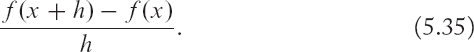
The above equation estimates the first-order derivative as the slope of a line joining the two points f(x) and f(x + h). The above expression is called the “Newton’s Difference Formula.”
Numerical differentiation is useful in cases where we know little about the underline real function or when the actual function is too complex. Also, in several cases we only have access to discrete sampled data (e.g., at different time instances) and a natural choice is to estimate the derivatives without necessarily modeling the function and calculating the exact derivatives. Numerical differentiation is fairly easy to implement, compared to other approaches. However, numerical differentiation provides only an estimate of the derivative and works poorly, particularly for the calculation of higher-order derivatives.
5.5.3 SYMBOLIC DIFFERENTIATION
Symbolic differentiation uses standard differential calculus formulas to manipulate mathematical expressions using computer algorithms. Popular softwares which perform symbolic differentiation include Mathematica, Maple, and Matlab.
Example: Suppose we are given a function f(x) = exp(sin(x)), we need to calculate its 10th derivative with respect to x. An analytical solution would be cumbersome, while a numerical solution will be less accurate. In such cases, we can effectively use symbolic differentiation to get a reliable answer. The following code in Matlab (using the Symbolic Math Toolbox) gives the desired result.
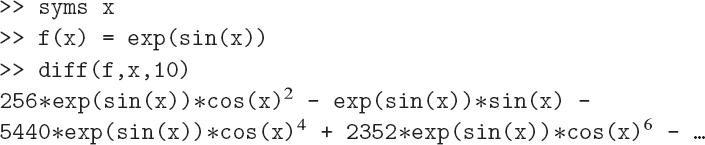
Symbolic differentiation, in a sense, is similar to analytical differentiation, but leveraging the power of computers to perform laborious derivations. This approach reduces the need to manually derive differentials and avoids the inaccuracies of numerical methods. However, symbolic differentiation often leads to complex and long expressions which results in slow software programs. Also, it does not scale well to higher-order derivatives (similar to numerical differentiation) due to the high complexity of the required computations. Furthermore, in neural network optimization, we need to calculate partial derivatives with respect to a large number of inputs to a layer. In such cases, symbolic differentiation is inefficient and does not scale well to large-scale networks.
5.5.4 AUTOMATIC DIFFERENTIATION
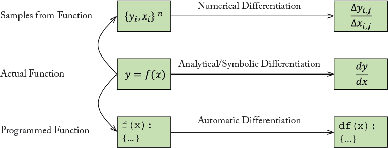
Automatic differentiation is a powerful technique which uses both numerical and symbolic techniques to estimate the differential calculation in the software domain, i.e., given a coded computer program which implements a function, automatic differentiation can be used to design another program which implements the derivative of that function. We illustrate the automatic differentiation and its relationship with the numerical and symbolic differentiation in Fig. 5.7.
Every computer program is implemented using a programming language, which only supports a set of basic functions (e.g., addition, multiplication, exponentiation, logarithm and trigonometric functions). Automatic differentiation uses this modular nature of computer programs to break them into simpler elementary functions. The derivatives of these simple functions are computed symbolically and the chain rule is then applied repeatedly to compute any order of derivatives of complex programs.
Automatic differentiation provides an accurate and efficient solution to the differentiation of complex expressions. Precisely, automatic differentiation gives results which are accurate to the machine precision. The computational complexity of calculating derivatives of a function is almost the same as evaluating the original function itself. Unlike symbolic differentiation, it neither needs a closed form expression of the function nor does it suffer from expression swell which renders symbolic differentiation inefficient and difficult to code. Current state of the art CNN libraries such as Theano and Tensorflow use automatic differentiation to compute derivatives (see Chapter 8).
Algorithm 5.1 Forward mode of Automatic Differentiation
Input: x, C
Output: yn
1: y0 ← x % initialization
2: for all i ∈ [1, n] do
3: ![]() % each function operates on its parents output in the graph
% each function operates on its parents output in the graph
4: end for
Algorithm 5.2 Backward mode of Automatic Differentiation
Input: x, C
![]()
1: Perform forward mode propagation
2: for all i ∈ [n – 1, 0] do
3: % chain rule to compute derivatives using child nodes in the graph
4: 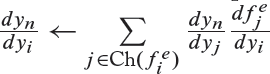
5: end for
6: ![]()
Automatic differentiation is very closely related to the back-propagation algorithm we studied before in Section 3.2.2. It operates in two modes, the forward mode and the backward mode. Given a complex function, we first decompose it into a computational graph consisting of simple elementary functions which are joined with each other to compute the complex function. In the forward mode, given an input x, the computational graph C with n intermediate states (corresponding to {fe}n elementary functions) can be evaluated sequentially as shown in Algorithm 5.1.
After the forward computations shown in Algorithm 5.1, the backward mode starts computing the derivatives toward the end and successively applies the chain rule to calculate the differential with respect to each intermediate output variable yi, as shown in Algorithm 5.2.
A basic assumption in the automatic differentiation approach is that the expression is differentiable. If this is not the case, automatic differentiation will fail. We provide a simple example of forward and backward modes of automatic differentiation below and refer the reader to Baydin et al. [2015] for a detailed treatment of this subject in relation to machine/deep learning techniques.
Example: Consider a slightly more complex function than the previous example for symbolic differentiation,
We can represent its analytically or symbolically calculated differential as follows:

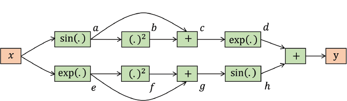
But, if we are interested in calculating its derivative using automatic differentiation, the first step would be to represent the complete function in terms of basic operations (addition, exp and sin) defined as:
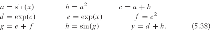
The flow of computations in terms of these basic operations is illustrated in the computational graph in Fig. 5.8. Given this computational graph we can easily calculate the differential of the output with respect to each of the variables in the graph as follows:
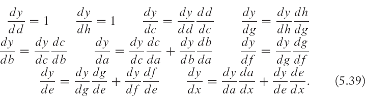
All of the above differentials can easily be computed because it is simple to compute the derivative of each basic function, e.g.,

Note that we started toward the end of the computational graph, and computed all of the intermediate differentials moving backward, until we got the differential with respect to input. The original differential expression we calculated in Eq. (5.37) was quite complex. However, once we decomposed the original expression in to simpler functions in Eq. (5.38), we note that the complexity of the operations that are required to calculate the derivative (back-ward pass) is almost the same as the calculation of the original expression (forward pass) according to the computational graph. Automatic differentiation uses the forward and backward operation modes to efficiently and precisely calculate the differentials of complex functions. As we discussed above, the operations for the calculation of differentials in this manner have a close resemblance to the back-propagation algorithm.
5.6 UNDERSTANDING CNN THROUGH VISUALIZATION
Convolutional networks are large-scale models with a huge number of parameters that are learned in a data driven fashion. Plotting an error curve and objective function on the training and validation sets against the training iterations is one way to track the overall training progress. However, this approach does not give an insight into the actual parameters and activations of the CNN layers. It is often useful to visualize what CNNs have learned during or after the completion of the training process. We outline some basic approaches to visualize CNN features and activations below. These approaches can be categorized into three types depending on the network signal that is used to obtain the visualization, i.e., weights, activations, and gradients. We summarize some of these three types of visualization methods below.
5.6.1 VISUALIZING LEARNED WEIGHTS
One of the simplest approaches to visualize what a CNN has learned is to look at the convolution filters. For example, 9 × 9 and 5 × 5 sized convolution kernels that are learned on a labeled shadow dataset are illustrated in Fig. 5.9. These filters correspond to the first and second convolutional layers in a LeNet style CNN (see Chapter 6 for details on CNN architectures).
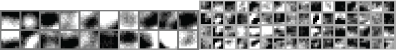
Figure 5.9: Examples of 9 × 9 (left) and 5 × 5 (right) sized convolution kernels learned for the shadow detection task. The filters illustrate the type of patterns that a particular CNN layer is looking for in the input data. (Figure adapted from Khan et al. [2014].)
The feature activations from the intermediate CNN layers can also provide useful clues about the quality of learned representations.
A trivial way to visualize learned features is to plot the output feature activations corresponding to an input image. As an example, we show the output convolutional activations (or features) corresponding to sample digits 2, 5, and 0 belonging to the MNIST dataset in Fig. 5.10. Specifically, these features are the output of the first convolution layer in the LeNet architecture (see Chapter 6 for details on this architecture type).
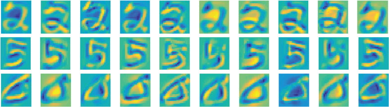
Figure 5.10: Intermediate feature representations from a CNN corresponding to example input images of handwritten digits from the MNIST dataset. Such a visualization of output activations can provide an insight about the patterns in input images that are extracted as useful features for classification.
Another approach is to obtain the feature representation from the penultimate layer of a trained CNN and visualize all the training images in a dataset as a 2D plot (e.g., using tSNE low dimensional embedding). The tSNE embedding approximately preserves the original distances in the high dimensional space between features. An example of such a visualization is shown in Fig. 5.11. This visualization can provide a holistic view and suggest the quality of learned feature representations for different classes. For instance, classes that are clustered tightly together in the feature space will be classified more accurately compared to the ones that have a widespread overlapping with other classes, making it difficult to accurately model the classification boundaries. Alongside visualizing 2D embedding of the high-dimensional feature vectors, we can also visualize the input images associated with each feature vector (see Fig. 5.13). In this manner, we can observe how visually similar images are clustered together in the tSNE embedding of high-dimensional features. As an example, cellar images are clustered together on the top left in the illustration shown in Fig. 5.13.
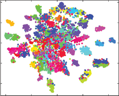
Figure 5.11: tSNE visualization of the final fully connected layer features corresponding to images from the MIT-67 indoor scene dataset. Each color represents a different class in the dataset. Note that the features belonging to the same class are clustered together. (Figure adapted from Khan et al. [2017b].)
An attention map can also provide an insight into the regions which were given more importance while making a classification decision. In other words, we can visualize the regions in an image which contributed most to the correct prediction of a category. One way to achieve this is to obtain prediction scores for individual overlapping patches with in an image and plot the final prediction score for the correct class. Examples of such a visualization is shown in Fig. 5.12. We can note that distinctive portions of the scenes played a crucial role in the correct prediction of the category for each image, e.g., a screen in an auditorium, train in a train station and bed in a bedroom.
Other interesting approaches have also been used in the literature to visualize the image parts which contribute most to the correct prediction. Zeiler and Fergus [2014] systematically occluded a square patch within an input image and plotted a heat map indicating the change in the prediction probability of the correct class. The resulting heat map indicates which regions in an input image are most important for a correct output response from the network (see Fig. 5.14a for examples). Bolei et al. [2015] first segments an input image into regions, these segments are then iteratively dropped such that the correct class prediction is least affected. This process continues until an image with minimal scene details is left. These details are sufficient for the correct classification of the input image (see Fig. 5.14b for examples).
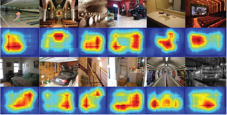
Figure 5.12: The contributions of distinctive patches with in an image toward the prediction of correct scene class are shown in the form of a heat map (“red” color denotes higher contribution). (Figure adapted from Khan et al. [2016b].)
5.6.3 VISUALIZATIONS BASED ON GRADIENTS
Balduzzi et al. [2017] presented the idea that visualizing distributions of gradients can provide useful insight into the convergence behavior of deep neural networks. Their analysis showed that naively increasing the depth of a neural network results in the gradient shattering problem (i.e., the gradients show similar distribution as white noise). They demonstrated that the gradient distribution resembled brown noise when batch normalization and skip connections were used in a very deep network (see Fig. 5.15).
Back-propagated gradients within a CNN have been used to identify specific patterns in the input image that maximally activate a particular neuron in a CNN layer. In other words, gradients can be adjusted to generate visualizations that illustrate the patterns that a neuron has learned to look for in the input data. Zeiler and Fergus [2014] pioneered this idea and introduced a deconvolution-based approach to invert the feature representations to identify associated patterns in the input images. Yosinski et al. [2015] generated synthetic images by first selecting an ith neuron in a CNN layer. Afterward, an input image with random color values is passed through the network and the corresponding activation value for ith neuron is calculated. The gradient of this activation with respect to the input image is calculated via error back propagation. This gradient basically denotes how the pixels can be changed such that the neuron gets maximally activated. The input gets iteratively modified using this information so that we obtain an image which results in a high activation for neuron i. Normally it is useful to impose a “style constraint” while modifying the input image which acts as a regularizer and enforces the input image to remain similar to the training data. Some example images thus obtained are shown in Fig. 5.16.

Figure 5.13: Visualization of images based on the tSNE embedding of the convolutional features from a deep network. The images belong to the MIT-67 dataset. Note that the images belonging to the same class are clustered together, e.g., all cellar images can be found in the top-left corner. (Figure adapted from Hayat et al. [2016].)
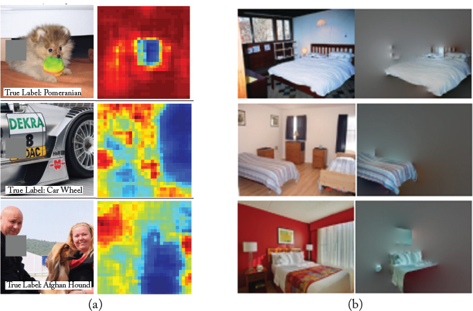
Figure 5.14: Visualization of regions which are important for the correct prediction from a deep network. (a) The grey regions in input images is sequentially occluded and the output probability of correct class is plotted as a heat map (blue regions indicate high importance for correct classification). (b) Segmented regions in an image are occluded until the minimal image details that are required for correct scene class prediction are left. As we expect, a bed is found to be the most important aspect of a bed-room scene. (Figures adapted from Bolei et al. [2015] and Zeiler and Fergus [2014], used “with permission.)
Mahendran and Vedaldi [2015] propose an approach to recover input images that correspond to identical high-dimensional feature representations in the second to last layer of CNN. Given an image x, a learned CNN F and a high dimensional representation f, the following loss is minimized through gradient descent optimization to find images in the input domain that correspond to the same feature representation f:
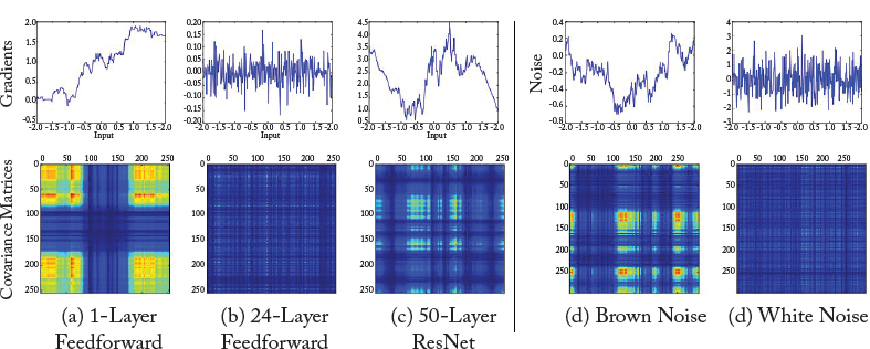
Figure 5.15: The top row shows the gradient distributions for a range of uniformly sampled inputs. The bottom row shows the covariance matrices. The gradient for the case of a 24 layered network resemble white noise, while the gradients of high-performing ResNet resemble brown noise. Note that the ResNet used skip connections and batch normalization which results in better converegence even with much deeper network architectures. The ResNet architecture will be discussed in detail in Chapter 6. (Figure from Balduzzi et al. [2017], used with permission.)
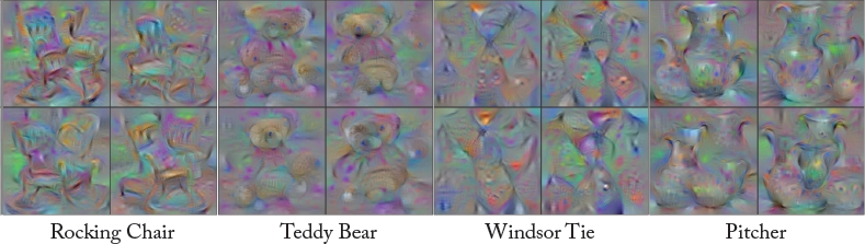
Figure 5.16: The figure illustrates synthetic input images that maximally activate the output neurons corresponding to different classes. As evident, the network looks for objects with similar low-level and high-level cues, e.g., edge information and holistic shape information, respectively, in order to maximally activate the relevant neuron. (Figure from Yosinski et al. [2015], used with permission.)
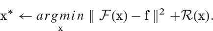
Here, R denotes a regularizer which enforces the generated images to look natural and avoid noisy and spiky patterns that are not helpful in perceptual visualization. Figure 5.17 illustrates examples of reconstructed images obtained from the CNN features at different layers of the network. It is interesting to note that the objects vary in position, scale and deformations but the holistic characteristics remain the same. This denotes that the network has learned meaningful characteristics of the input image data.
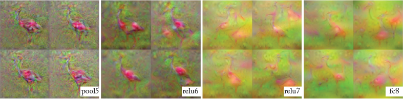
Figure 5.17: Multiple inverted images obtained from the high dimensional feature representations of a CNN. Note that the features from lower layers retain local information better than the higher ones. (Figure from Mahendran and Vedaldi [2015], used with permission.)
Up to this point, we have completed the discussion about the CNN architecture, its training process and the visualization approaches to understand the working of CNNs. Next, we will describe a number of successful CNN examples from the literature which will help us develop an insight into the state-of-the-art network topologies and their mutual pros and cons.