Neural Networks Basics
Before going into the details of the CNNs, we provide in this chapter an introduction to artificial neural networks, their computational mechanism, and their historical background. Neural networks are inspired by the working of cerebral cortex in mammals. It is important to note, however, that these models do not closely resemble the working, scale and complexity of the human brain. Artificial neural network models can be understood as a set of basic processing units, which are tightly interconnected and operate on the given inputs to process the information and generate desired outputs. Neural networks can be grouped into two generic categories based on the way the information is propagated in the network.
• Feed-forward networks
The information flow in a feed-forward network happens only in one direction. If the network is considered as a graph with neurons as its nodes, the connections between the nodes are such that there are no loops or cycles in the graph. These network architectures can be referred as Directed Acyclic Graphs (DAG). Examples include MLP and CNNs, which we will discuss in details in the upcoming sections.
• Feed-back networks
As the name implies, feed-back networks have connections which form directed cycles (or loops). This architecture allows them to operate on and generate sequences of arbitrary sizes. Feed-back networks exhibit memorization ability and can store information and sequence relationships in their internal memory. Examples of such architectures include Recurrent Neural Network (RNN) and Long-Short Term Memory (LSTM).
We provide an example architecture for both feed-forward and feed-back networks in Sections 3.2 and 3.3, respectively. For feed-forward networks, we first study MLP, which is a simple case of such architectures. In Chapter 4, we will cover the CNNs in detail, which also work in a feed-forward manner. For feed-back networks, we study RNNs. Since our main focus here is on CNNs, an in-depth treatment of RNNs is out of the scope of this book. We refer interested readers to Graves et al. [2012] for RNN details.
Figure 3.1 shows an example of a MLP network architecture which consists of three hidden layers, sandwiched between an input and an output layer. In simplest terms, the network can be treated as a black box, which operates on a set of inputs and generates some outputs. We highlight some of the interesting aspects of this architecture in more details below.
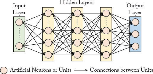
Layered Architecture: Neural networks comprise a hierarchy of processing levels. Each level is called a “network layer” and consists of a number of processing “nodes” (also called “neurons” or “units”). Typically, the input is fed through an input layer and the final layer is the output layer which makes predictions. The intermediate layers perform the processing and are referred to as the hidden layers. Due to this layered architecture, this neural network is called an MLP.
Nodes: The individual processing units in each layer are called the nodes in a neural network architecture. The nodes basically implement an “activation function” which given an input, decides whether the node will fire or not.
Dense Connections: The nodes in a neural network are interconnected and can communicate with each other. Each connection has a weight which specifies the strength of the connection between two nodes. For the simple case of feed-forward neural networks, the information is transferred sequentially in one direction from the input to the output layers. Therefore, each node in a layer is directly connected to all nodes in the immediate previous layer.
As we described in Section 3.2.1, the weights of a neural network define the connections between neurons. These weights need to be set appropriately so that a desired output can be obtained from the neural network. The weights encode the “model” generated from the training data that is used to allow the network to perform a designated task (e.g., object detection, recognition, and/or classification). In practical settings, the number of weights is huge which requires an automatic procedure to update their values appropriately for a given task. The process of automatically tuning the network parameters is called “learning” which is accomplished during the training stage (in contrast to the test stage where inference/prediction is made on “unseen data,” i.e., data that the network has not “seen” during training). This process involves showing examples of the desired task to the network so that it can learn to identify the right set of relationships between the inputs and the required outputs. For example, in the paradigm of supervised learning, the inputs can be media (speech, images) and the outputs are the desired set of “labels” (e.g., identity of a person) which are used to tune the neural network parameters.
We now describe a basic form of learning algorithm, which is called the Delta Rule.
Delta Rule
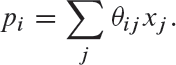
The basic idea behind the delta rule is to learn from the mistakes of the neural network during the training phase. The delta rule was proposed by Widrow et al. [1960], which updates the network parameters (i.e., weights denoted by θ, considering 0 biases) based on the difference between the target output and the predicted output. This difference is calculated in terms of the Least Mean Square (LMS) error, which is why the delta learning rule is also referred to as the LMS rule. The output units are a “linear function” of the inputs denoted by x, i.e.,
If pn and yn denote the predicted and target outputs, respectively, the error can be calculated as:
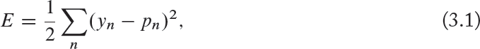
where n is the number of categories in the dataset (or the number of neurons in the output layer). The delta rule calculates the gradient of this error function (Eq. (3.1)) with respect to the parameters of the network: ∂E/∂θij. Given the gradient, the weights are updated iteratively according to the following learning rule:

where t denotes the previous iteration of the learning process. The hyper-parameter η) denotes the step size of the parameter update in the direction of the calculated gradient. One can visualize that no learning happens when the gradient or the step size is zero. In other cases, the parameters are updated such that the predicted outputs get closer to the target outputs. After a number of iterations, the network training process is said to converge when the parameters do not change any longer as a result of the update.
If the step size is unnecessarily too small, the network will take longer to converge and the learning process will be very slow. On the other hand, taking very large steps can result in an unstable erratic behavior during the training process as a result of which the network may not converge at all. Therefore, setting the step-size to a right value is really important for network training. We will discuss different approaches to set the step size in Section 5.3 for CNN training which are equally applicable to MLP.
Generalized Delta Rule
The generalized delta rule is an extension of the delta rule. It was proposed by Rumelhart et al. [1985]. The delta rule only computes linear combinations between the input and the output pairs. This limits us to only a single-layered network because a stack of many linear layers is not better than a single linear transformation. To overcome this limitation, the generalized delta rule makes use of nonlinear activation functions at each processing unit to model nonlinear relationships between the input and output domains. It also allows us to make use of multiple hidden layers in the neural network architecture, a concept which forms the heart of deep learning.
The parameters of a multi-layered neural network are updated in the same manner as the delta rule, i.e.,

But different to the delta rule, the errors are recursively sent backward through the multi-layered network. For this reason, the generalized delta rule is also called the “back-propagation” algorithm. Since for the case of the generalized delta rule, a neural network not only has an output layer but also intermediate hidden layers, we can separately calculate the error term (differential with respect to the desired output) for the output and hidden layers. Since the case of the output layer is simple, we first discuss the error computation for this layer.
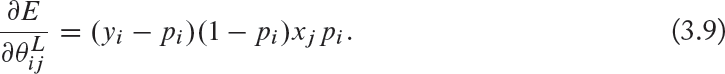
Given the error function in Eq. (3.1), its gradient with respect to the parameters in the output layer L for each node i can be computed as follows:

where, ![]() is the activation which is the input to the neuron (prior to the activation function), xj’s are the outputs from the previous layer, pi = f(ai) is the output from the neuron (prediction for the case of output layer) and f(·) denotes a nonlinear activation function while f′(·) represents its derivative. The activation function decides whether the neuron will fire or not, in response to a given input activation. Note that the nonlinear activation functions are differentiable so that the parameters of the network can be tuned using error back-propagation.
is the activation which is the input to the neuron (prior to the activation function), xj’s are the outputs from the previous layer, pi = f(ai) is the output from the neuron (prediction for the case of output layer) and f(·) denotes a nonlinear activation function while f′(·) represents its derivative. The activation function decides whether the neuron will fire or not, in response to a given input activation. Note that the nonlinear activation functions are differentiable so that the parameters of the network can be tuned using error back-propagation.
One popular activation function is the sigmoid function, given as follows:

We will discuss other activation functions in detail in Section 4.2.4. The derivative of the sigmoid activation function is ideally suitable because it can be written in terms of the sigmoid function itself (i.e., pi) and is given by:
Therefore, we can write the gradient equation for the output layer neurons as follows:
Similarly, we can calculate the error signal for the intermediate hidden layers in a multi-layered neural network architecture by back propagation of errors as follows:

where l ∈ {1 … L – 1} and L denotes the total number of layers in the network. The above equation applies the chain rule to progressively calculate the gradients of the internal parameters using the gradients of all subsequent layers. The overall update equation for the MLP parameters θij can be written as:
where ![]() is the output from the previous layer and t denotes the number of previous training iteration. The complete learning process usually involves a number of iterations and the parameters are continually updated until the network is optimized (i.e., after a set number of iterations or when
is the output from the previous layer and t denotes the number of previous training iteration. The complete learning process usually involves a number of iterations and the parameters are continually updated until the network is optimized (i.e., after a set number of iterations or when ![]() does not change).
does not change).
Gradient Instability Problem: The generalized delta rule successfully works for the case of shallow networks (ones with one or two hidden layers). However, when the networks are deep (i.e., L is large), the learning process can suffer from the vanishing or exploding gradient problems depending on the choice of the activation function (e.g., sigmoid in above example). This instability relates particularly to the initial layers in a deep network. As a result, the weights of the initial layers cannot be properly tuned. We explain this with an example below.
Consider a deep network with many layers. The outputs of each weight layer are squashed within a small range using an activation function (e.g., [0,1] for the case of the sigmoid). The gradient of the sigmoid function leads to even smaller values (see Fig. 3.2). To update the initial layer parameters, the derivatives are successively multiplied according to the chain rule (as in Eq. (3.10)). These multiplications exponentially decay the back-propagated signal. If we consider a network depth of 5, and the maximum possible gradient value for the sigmoid (i.e., 0.25), the decaying factor would be (0.25)5 = 0.0009. This is called the “vanishing gradient” problem. It is easy to follow that in cases where the gradient of the activation function is large, successive multiplications can lead to the “exploding gradient” problem.
We will introduce the ReLU activation function in Chapter 4, whose gradient is equal to 1 (when a unit is “on”). Since 1L = 1, this avoids both the vanishing and the exploding gradient problems.
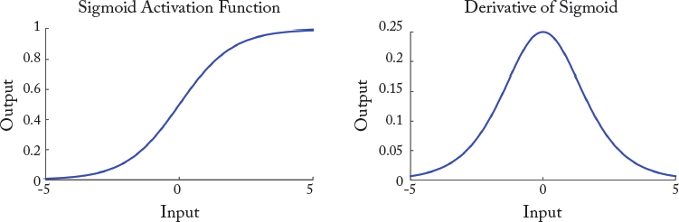
Figure 3.2: The sigmoid activation function and its derivative. Note that the range of values for the derivative is relatively small which leads to the vanishing gradient problem.
The feed-back networks contain loops in their network architecture, which allows them to process sequential data. In many applications, such as caption generation for an image, we want to make a prediction such that it is consistent with the previously generated outputs (e.g., already generated words in the caption). To accomplish this, the network processes each element in an input sequence in a similar fashion (while considering the previous computational state). For this reason it is also called an RNN.
Since, RNNs process information in a manner that is dependent on the previous computational states, they provide a mechanism to “remember” previous states. The memory mechanism is usually effective to remember only the short term information that is previously processed by the network. Below, we outline the architectural details of an RNN.
A simple RNN architecture is shown in Fig. 3.3. As described above, it contains a feed-back loop whose working can be visualized by unfolding the recurrent network over time (shown on the right). The unfolded version of the RNN is very similar to a feed-forward neural network described in Section 3.2. We can, therefore, understand RNN as a simple multi-layered neural network, where the information flow happens over time and different layers represent the computational output at different time instances. The RNN operates on sequences and therefore the input and consequently the output at each time instance also varies.
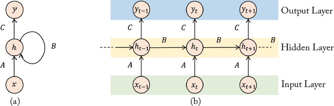
Figure 3.3: The RNN Architecture. Left: A simple recurrent network with a feed-back loop. Right: An unfolded recurrent architecture at different time-steps.
We highlight the key features of an RNN architecture below.
Variable Length Input: RNN can operate on inputs of variable length, e.g., videos with variable frame length, sentences with different number of words, 3D point clouds with variable number of points. The length of the unfolded RNN structure depends on the length of the input sequence, e.g., for a sentence consisting of 12 words, there will be a total of 12 layers in the unfolded RNN architecture. In Fig. 3.3, the input to the network at each time instance t is represented by the variable xt.
Hidden State: The RNN holds internally the memory of the previous computation in a hidden state represented by ht. This state can be understood as an input from the previous layer in the unfolded RNN structure. At the beginning of the sequence processing, it is initialized with a zero or a random vector. At each time step, this state is updated by considering its previous value and the current input to the network:
where f(·) is the nonlinear activation function. The weight matrix B is called the transition matrix since it influences how the hidden state changes over time.
Variable Length Output: The output of RNN at each time step is denoted by yt. The RNNs are capable of generating variable length outputs, e.g., translating a sentence in one language to another language where the output sequence lengths can be different from the input sequence length. This is possible because RNNs consider the hidden state while making predictions. The hidden state models the joint probability of the previously processed sequence which can be used to predict new outputs. As an example, given a few starting words in a sentence, the RNN can predict the next possible word in the sentence, where a special end of a sentence symbol is used to denote the end of each sentence. In this case all possible words (including the end of sentence symbol) are included in the dictionary over which the prediction is made:
where f(·) is an activation function such as a softmax (Section 4.2.4).
Shared Parameters: The parameters in the unfolded RNN linking the input, the hidden state and the output (denoted by A, B, and C, respectively) are shared between all layers. This is the reason why the complete architecture can be represented by using a loop to represent its recurrent architecture. Since the parameters in a RNN are shared, the total number of tunable parameters are considerably less than an MLP, where a separate set of parameters are learned for each layer in the network. This enables efficient training and testing of the feed-back networks.
Based on the above description of RNN architecture, it can be noted that indeed the hidden state of the network provides a memory mechanism, but it is not effective when we want to remember long-term relationships in the sequences. Therefore, RNN only provide short-term memory and find difficulties in “remembering” (a few time-steps away) old information processed through it. To overcome this limitation, improved versions of recurrent networks have been introduced in the literature which include the LSTM [Hochreiter and Schmidhuber, 1997], Gated Recurrent Unit (GRU) [Cho et al., 2014], Bi-directional RNN (B-RNN) [Graves and Schmidhuber, 2005] and Neural Turing Machines (NTM) [Graves et al., 2014]. However, the details of all these network architectures and their functioning is out of the scope of this book which is focused on feed-forward architectures (particularly CNNs).
The parameters in a feed-back network can be learned using the generalized delta rule (back-propagation algorithm), similar to feed-forward networks. However, instead of error back-propagation through network layers as in feed-forward networks, back-propagation is performed through time in the feed-back networks. At each time instance, the output of the RNN is computed as a function of its previous and current inputs. The Back Propagation Through Time (BPTT) algorithm cannot allow the learning of long-term relationships in sequences, because of difficulties in error computations over long sequences. Specifically, when the number of iterations increases, the BPTT algorithm suffers from the vanishing or the exploding gradient problem. One way around this problem is to compute the error signal over a truncated unfolded RNN. This reduces the cost of the parameter update process for long sequences, but limits the dependence of the output at each time instance to only few previous hidden states.
3.4 LINK WITH BIOLOGICAL VISION
We think it is important to briefly discuss biological neural networks (BNNs) and their operational mechanisms in order to study their similarities and dissimilarities with artificial neural networks. As a matter of fact, artificial neural networks do not resemble their biological counterparts in terms of functioning and scale, however they are indeed motivated by the BNNs and several of the terms used to describe artificial neural networks are borrowed from the neuroscience literature. Therefore, we introduce neural networks in the brain, draw parallels between artificial and biological neurons, and provide a model of the artificial neuron based on biological vision.
The human brain contains approximately 100 billion neurons. To interpret this number, let us assume we have 100 billion one dollar bills, where each bill is only 0.11 mm thick. If we stack all these one dollar bills on top of each other, the resulting stack will be 10922.0 km high. This illustrates the scale and magnitude of the human brain.
A biological neuron is a nerve cell which processes information [Jain et al., 1996]. Each neuron is surrounded by a membrane and has a nucleus which contains genes. It has specialized projections which manage the input and output to the nerve cell. These projections are termed dendrites and axons. We describe these and other key aspects of the biological neuron below.
Dendrites: Dendrites are fibers which act as receptive lines and bring information (activations) to the cell body from other neurons. They are the inputs of the neuron.
Axons: Axons are fibers which act as transmission lines and take information away from the cell body to other neurons. They act as outputs of the neuron.
Cell body: The cell body (also called the soma) receives the incoming information through dendrites, processes it and sends it, to other neurons via axons.
Synapses: The specialized connections between axons and dendrites which allow the communication of signals are called synapses. The communication takes place by an electro-chemical process where the neurotransmitters (chemicals) are released at the synapse and are diffused across the synaptic gap to transmit information. There is a total of approximately 1 quadrillion (1015) synapses in the human brain [Changeux and Ricoeur, 2002].
Connections: Neurons are densely inter-connected with each other. On average, each neuron receives inputs from approximately 105 synapses.
Neuron Firing: A neuron receives signals from connected neurons via dendrites. The cell body sums up the received signals and the neuron fires if the combined input signal exceeds a threshold. By neuron firing, we mean that it generates an output which is sent out through axons. If the combined input is below the threshold, no response signal is generated by the neuron (i.e., the neuron does not fire). The thresholding function which decides whether a neuron fires or not is called activation function.
Next, we describe a simple computational model which mimics the working of a biological neuron.
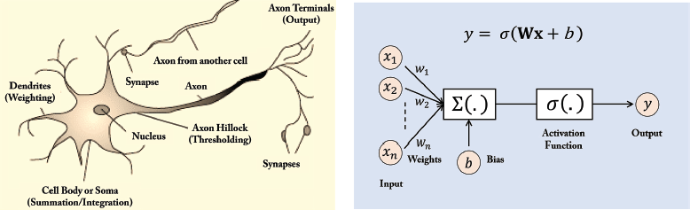
Figure 3.4: A biological neuron (left) and a computational model (right) which is used to develop artificial neural networks.
3.4.2 COMPUTATIONAL MODEL OF A NEURON
A simple mathematical model of the biological neuron known as the Threshold Logic Unit (TLU) was proposed by McCulloch and Pitts [1943]. It consists of a set of incoming connections which feed the unit with activations coming from other neurons. These inputs are weighted using a set of weights denoted by {w}. The processing unit then sums all the inputs and applies a nonlinear threshold function (also known as the activation function) to calculate the output. The resulting output is then transmitted to other connected neural units. We can denote the operation of a McCulloch-Pitts neuron as follows:

where b is a threshold, wi denote the synapse weight, xi is the input to the neuron, and f(·) represents a nonlinear activation function. For the simplest case, f is a step function which gives 0 (i.e., neuron does not fire) when the input is below 0 (i.e., ![]() less than the firing threshold) and 1 when it is greater than 0. For other cases, the activation function can be a sigmoid, tanh, or an ReLU for a smooth thresholding operation (see Chapter 4).
less than the firing threshold) and 1 when it is greater than 0. For other cases, the activation function can be a sigmoid, tanh, or an ReLU for a smooth thresholding operation (see Chapter 4).
The McCulloch-Pitts neuron is a very simple computational model. However, they have been shown to approximate complex functions quite well. McCulloch and Pitts showed that a network comprising of such neurons can perform universal computations. The universal computational ability of neural networks ensures their ability to model a very rich set of continuous functions using only a finite number of neurons. This fact is formally known as the “Universal Approximation Theorem” for neural networks. Different to McCulloch-Pitts model, state of the art neuron models also incorporate additional features such as stochastic behaviors and non-binary input and output.
3.4.3 ARTIFICIAL VS. BIOLOGICAL NEURON
Having outlined the basics of artificial and biological neuron operation, we can now draw parallels between their functioning and identify the key differences between the two.
An artificial neuron (also called a unit or a node) takes several input connections (dendrites in biological neuron) which are assigned certain weights (analogous to synapses). The unit then computes the sum of the weighted inputs and applies an activation function (analogous to the cell body in biological neuron). The result of the unit is then passed on using the output connection (axon function).
Note that the above-mentioned analogy between a biological and an artificial neuron is only valid in the loose sense. In reality, there exists a number of crucial differences in the functioning of biological neurons. As an example, biological neurons do not sum the weighted inputs, rather dendrites interact in a much complex way to combine the incoming information. Furthermore, biological neurons communicate asynchronously, different from their computational counterparts which operate synchronously. The training mechanisms in both types of neural networks are also different, while the training mechanisms in biological networks are not precisely known. The topology in biological networks are very complicated compared to the artificial networks which currently have either a feed-forward or feed-back architecture.