Applications of CNNs in Computer Vision
Computer vision is a very broad research area which covers a wide variety of approaches not only to process images but also to understand their contents. It is an active research field for convolutional neural network applications. The most popular of these applications include, classification, segmentation, detection, and scene understanding. Most CNN architectures have been used for computer vision problems including, supervised or unsupervised face/object classification (e.g., to identify an object or a person in a given image or to output the class label of that object), detection (e.g., annotate an image with bounding boxes around each object), segmentation (e.g., labeling pixels of an input image), and image generation (e.g., converting low-resolution images to high resolution ones). In this chapter, we describe various applications of convolutional neural networks in computer vision. Note that this chapter is not a literature review, it rather provides a description of representative works in different areas of computer vision.
CNNs have been shown to be an effective tool for the task of image classification [Deng, 2014]. For instance, in the 2012 ImageNet LSVRC contest, the first large-scale CNN model, which was called AlexNet [Krizhevsky et al., 2012] (Section 6.2), achieved considerably lower error rates compared to the previous methods. ImageNet LSVRC is a challenging contest as the training set consists of about 1.2 million images belonging to 1,000 different classes, while the test set has around 150,000 images. After that, several CNN models (e.g., VGGnet, GoogleNet, ResNet, DenseNet) have been proposed to further decrease the error rate. While Chapter 6 has already introduced these state-of-the art CNN models for image classification task, we will discuss below a more recent and advanced architecture, which was proposed for 3D point cloud classification (input to the model is a raw 3D point cloud) and achieved a high classification performance.
PointNet [Qi et al., 2016] is a type of neural network which takes orderless 3D point clouds as input and well respects the permutation invariance of the input points. More precisely, PointNet approximates a set function g defined on an orderless 3D point cloud, {x1, x2, …, xn}, to map the point cloud to a vector:
where γ and h are multi-layer perceptron (mlp) networks. Thus, the set function g is invariant to the permutation of the input points and can approximate any continuous set function [Qi et al., 2016].
PointNet, shown in Fig. 7.1, can be used for classification, segmentation, and scene semantic parsing from point clouds. It directly takes an entire point cloud as input and outputs a class label to accomplish 3D object classification. For segmentation, the network returns perpoint labels for all points within the input point cloud. PointNet has three main modules, which we briefly discuss below.
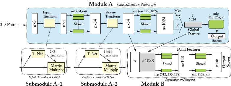
Figure 7.1: PointNet architecture: The input to classification network (Module A) are 3D point clouds. The network applies a sequence of non-linear transformations, including input and feature transformations (Submodule A-1), and then uses max-pooling to aggregate point features. The output is a classification score for C number of classes. The classification network can be extended to form the segmentation network (Module B). “mlp” stands for multi-layered perceptron and numbers in bracket are layer sizes.
Classification Network (Module A):
The first key module of PointNet is the classification network (module A), shown in Fig. 7.1. This module consists of input (Submodule A-1) and feature (Submodule A-2) transformation networks, multi-layer perceptrons (mlp) networks, and a max-pooling layer. Each point within the orderless input point cloud ({x1, x2, …, xn}) is first passed through two shared mlp networks (function h(·) in Eq. (7.1)) to transfer 3D points to a high dimensional, e.g., 1024-dimensional, feature space. Next, the max-pooling layer (function max(·) in Eq. (7.1)) is used as a symmetric function to aggregate information from all the points, and to make a model invariant to input permutations. The output of the max-pooling layer ![]() in Eq. (7.1)) is a vector, which represents a global shape feature of the input point cloud. This global feature is then passed through an mlp network followed by a soft-max classifier (function γ(·) in Eq. (7.1)) to assign a class label to the input point cloud.
in Eq. (7.1)) is a vector, which represents a global shape feature of the input point cloud. This global feature is then passed through an mlp network followed by a soft-max classifier (function γ(·) in Eq. (7.1)) to assign a class label to the input point cloud.
Transformation/Alignment Network (Submodule A-1 and Submodule A-2):
The second module of PointNet is the transformation network (mini-network or T-net in Fig. 7.1), which consists of a a shared mlp network, that is applied on each point, followed by a max-pooling layer which is applied across all points and two fully connected layers. This network predicts an affine transformation to ensure that the semantic labeling of a point cloud is invariant to geometric transformations. As shown in Fig. 7.1, there are two different transformation networks, including the input (Submodule A-1) and the feature transformation (Submodule A-2) networks. The input 3D points are first passed through the input transformation network to predict a 3 × 3 affine transformation matrix. Then, new per-point features are computed by applying the affine transformation matrix to the input point cloud (“Matrix multiply” box in Submodule A-1).
The feature transform network is a replica of the input transform network, shown in Fig. 7.1 (Submodule A-2), and is used to predict the feature transformation matrix. However, unlike the input transformation network, the feature transformation network takes 64-dimensional points. Thus, its predicted transformation matrix has a dimension of 64 × 64, which is higher than the input transformation matrix (i.e., 3 × 3 in Submodule A-1). This contributes to the difficulty of achieving optimization. To address this problem, a regularization term is added to the soft-max loss to constrain the 64 × 64 feature transformation matrix to be close to an orthogonal matrix:
where A is the feature transformation matrix.
Segmentation Network (Module B):
PointNet can be extended to predict per point quantities, which rely on both the local geometry and the global semantics. The global feature computed by the classification network (Module A) is fed to the segmentation network (Module B). The segmentation network combines the global and per-point point features, and then passed them through an mlp network to extract new per-point features. These new features contain both the global and local information, which has shown to be essential for segmentation [Qi et al., 2016]. Finally, the point features are passed through a shared mlp layer to assign a label to each point.
7.2 OBJECT DETECTION AND LOCALIZATION
Recognizing objects and localizing them in images is one of the challenging problems in computer vision. Recently, several attempts have been made to tackle this problem using CNNs. In this section, we will discuss three recent CNN-based techniques, which were used for detection and localization.
In Girshick et al. [2016], Region-based CNN (R-CNN) has been proposed for object detection. It will be good to give here the broad idea behind R-CNN, i.e., region wise feature extraction using deep CNNs and the learning of independent linear classifiers for each object class. The R-CNN object detection system consists of the following three modules.
Regional Proposals (Module A in Fig. 7.2) and Feature Extraction (Module B)
Given an image, the first module (Module A in Fig. 7.2) uses selective search [Uijlings et al., 2013] to generate category-independent region proposals, which represent the set of candidate detections available to the object detector.
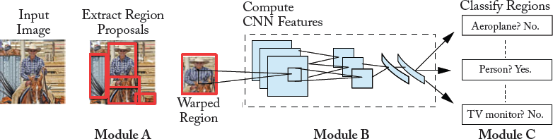
Figure 7.2: RCNN object detection system. Input to R-CNN is an RGB image. It then extracts region proposals (Module A), computes features for each proposal using a deep CNN, e.g., AlexNet (Module B), and then classifies each region using class-specific linear SVMs (Module
The second module (Module B in Fig. 7.2) is a deep CNN (e.g., AlexNet or VGGnet), which is used to extract a fixed-length feature vector from each region. In both cases (AlexNet or VGGnet), the feature vectors are 4096-dimensional. In order to extract features from a region of a given image, the region is first converted to make it compatible with the network input. More precisely, irrespective of the candidate region’s aspect ratio or size, all pixels are converted to the required size by warping them in a tight bounding box. Next, features are computed by forward propagating a mean-subtracted RGB image through the network and reading off the output values by the last fully connected layer just before the soft-max classifier.
Training Class Specific SVMs (Module C)
After feature extraction, one linear SVM per class is learned, which is the third module of this detection system. In order to assign labels to training data, all region proposals with an overlap greater than or equal to 0.5 IoU with a ground-truth box are considered as positives for the class of that box, while the rest are considered as negatives. Since the training data is very large for the available memory, the standard hard negative mining method [Felzenszwalb et al., 2010] is used to achieve quick convergence.
Pre-training and Domain Specific Training of Feature Extractor
For the pre-training of the CNN feature extractor, a large ILSVRC2012 classification dataset with image-level annotations is used. Next, SGD training with the warped region proposals is performed for adaptation of the network to the new domain and the new task of image detection. The network architecture is kept unchanged except for a 1000-way classification layer, which is set to 20+1 for PASCAL VOC and to 200+1 for ILSVRC2013 datasets (equal to the number of classes in these datasets + background).
R-CNN Testing
At test time, a selective search is run to select 2,000 region proposals from the test image. To extract features from these regions, each one of them is warped and then forward propagated through the learned CNN feature extractor. SVM trained for each class is then used to score the feature vectors of each class. Once all these regions have been scored, a greedy non-maximum suppression is used to reject a proposal, which has an IoU overlap with a higher scoring selected region greater than a pre-specified threshold. R-CNN has been shown to improve the mean average precision (mAP) by a significant margin.
R-CNN Drawbacks
The R-CNN discussed above achieves an excellent object detection accuracy. However, it still has few drawbacks. The training of R-CNN is multi-staged. In the case of R-CNN, soft-max loss is employed to fine tune the CNN feature extractor (e.g., AlexNet, VGGnet) on object proposals. SVM are next fitted to the network’s features. The role of SVMs is to perform object detection and replace the soft-max classifier. In terms of complexity in time and space, the training of this model is computationally expensive. This is because, every region proposal is required to pass through the network. For example, training VGGnet-16 on 5,000 images of the PASCAL VOC07 dataset using a GPU takes 2.5 days. In addition, the extracted features need a huge storage, i.e., hundreds of gigabytes. R-CNN is also slow in performing object detection at test time. For example, using VGGnet-16 (on a GPU) as the feature extractor in Module B, detection of an object takes around 47 seconds per image. To overcome these problems, an extension of R-CNN called the Fast R-CNN was proposed.
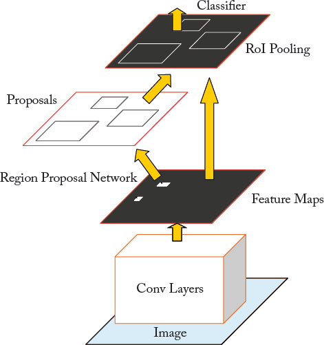
Figure 7.3 shows the Fast R-CNN model. The input to Fast R-CNN is an entire image along with object proposals, which are extracted using the selective search algorithm [Uijlings et al., 2013]. In the first stage, convolutional feature maps (usually feature maps of the last convolutional layer) are extracted by passing the entire image through a CNN, such as AlexNet and VGGnet (Module A in Fig. 7.3). For each object proposal, a feature vector of fixed size is then extracted from the feature maps by a Region of Interest (RoI) pooling layer (Module B), which has been explained in Section 4.2.7. The role of the RoI pooling layer is to convert the features, in a valid RoI, into small feature maps of fixed size (X × Y, e.g., 7 × 7), using max-pooling. X and Y are the layer hyper-parameters. A RoI itself is a rectangular window which is characterized by a 4-tuple that defines its top-left corner (a, b) and its height and width (x, y). The RoI layer divides the RoI rectangular area of size x × y into an X × Y grid of sub-windows, which has a size of x/X × y/Y. The values in each sub-window are then max-pooled into the corresponding output grid. Note that the max-pooling operator is applied independently to each convolutional feature map. Each feature vector is then given as input to fully connected layers, which branch into two sibling output layers. One of these sibling layers (Module C in Fig. 7.3) gives estimates of the soft-max probability over object classes and a background class. The other layer (Module D in Fig. 7.3) produces four values, which redefine bounding box positions, for each of the object classes.

Figure 7.3: Fast R-CNN Architecture. The input to a fully convolutional network (e.g., AlexNet) is an image and RoIs (Module A). Each RoI is pooled into a fixed-size feature map (Module B) and then passed through the two fully-connected layers to form a RoI feature vector. Finally, the RoI feature vector is passed through two sibling layers, which output the soft-max probability over different classes (Module C) and bounding box positions (Module D).
Fast R-CNN Initialization and Training
Fast R-CNN is initialized from three pre-trained ImageNet models including: AlexNet [Krizhevsky et al., 2012], VGG-CNN-M-1024 [Chatfield et al., 2014], and VGGnet-16 [Simonyan and Zisserman, 2014b] models. During initialization, a Fast R-CNN model undergoes three transformations. First, a RoI pooling layer (Module B) replaces the last max-pooling layer to make it compatible with the network’s first fully connected layer (e.g., for VGGnet-16 X = Y = 7). Second, the two sibling layers ((Module C and Module D), discussed above, replace the last fully connected layer and soft-max of the network. Third, the network model is tweaked to accept two data inputs, i.e., a list of images and their RoIs. Then SGD simultaneously optimizes the soft-max classifier (Module C) and the bounding-box regressor (Module D) in an end-to-end fashion by using a multi-task loss on each labeled RoI.
Detection Using Fast R-CNN
For detection, the Fast R-CNN takes as an input, an image along with a list of R object proposals to score. During testing, R is kept at around 2,000. For each test RoI(r), the class probability score for each of the K classes (module C in Fig. 7.3) and a set of refined bounding boxes are computed (module D in Fig. 7.3). Note that each of the K classes has its own refined bounding box. Next, the algorithm and the configurations from R-CNN are used to independently perform non-maximum suppression for each class. Fast R-CNN has been shown to achieve a higher detection performance (with a mAP of 66% compared to 62% for R-CNN) and computational efficiency on PASCAL VOC 2012 dataset. The training of Fast R-CNN, using VGGnet-16, was 9× faster than R-CNN and this network was found 213 × faster at test-time.
While Fast R-CNN has increased the training and testing speed of R-CNN by sharing a single CNN computation across all region proposals, its computational efficiency is bounded by the speed of the region proposal methods, which are run on CPUs. The straightforward approach to address this issue is to implement region proposal algorithms on GPUs. Another elegant way is to rely on algorithmic changes. In the following section, we discuss an architecture, known as Regional Proposal Network [Ren et al., 2015], which relies on an algorithmic change by computing nearly cost-free region proposals with CNN in an end-to-end learning fashion.
7.2.3 REGIONAL PROPOSAL NETWORK (RPN)
The Regional Proposal Network [Ren et al., 2015] (Fig. 7.4) simultaneously predicts object bounding boxes and objectness scores at each position. RPN is a fully convolutional network, which is trained in an end-to-end fashion, to produce high quality region proposals for object detection using Fast R-CNN (described in Section 7.2.2). Combining RPN with Fast R-CNN object detector results in a new model, which is called Faster R-CNN (shown in Fig. 7.5). Notably, in Faster R-CNN, the RPN shares its computation with Fast R-CNN by sharing the same convolutional layers, allowing for joint training. The former has five, while the later has 13 shareable convolutional layers. In the following, we first discuss the RPN and then Faster R-CNN, which merges RPN and Fast R-CNN into a single network.
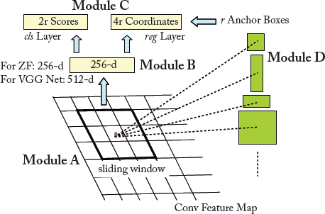
Figure 7.4: Regional proposal network (RPN) architecture, which is illustrated at a single position.
The input to the RPN is an image (re-scaled in such a way that its smaller side is equal to 600 pixels) and the output is a set of object bounding boxes and associated objectness scores (as shown in Fig. 7.4). To generate region proposals with RPN, the image is first passed through the shareable convolutional layers. A small spatial window (e.g., 3 × 3) is then slid over the output feature maps of the last shared convolutional layer, e.g., conv5 for VGGnet-16 (Module A in Fig. 7.4). This sliding window at each position is then transformed to a lower-dimensional vector of size 256-d and 512-d for ZF and VGGnet-16 models (Module B in Fig. 7.4), respectively. Next, this vector is given as an input to two sibling fully connected layers, including the bounding box regression layer (reg) and the bounding box classification layer (cls) (Module C in Fig. 7.4). In summary, the above-mentioned steps (Module A, Module B, and Module C) can be implemented with a 3 × 3 convolutional layer followed by two sibling 1 × 1 convolutional layers.
Multi-scale Region Proposal Detection
Unlike image/feature pyramid-based methods, such as the spatial pyramid pooling (SPP) layer [He et al., 2015b] (discussed in Section 4.2.8), which uses time-consuming feature pyramids in convolutional feature maps, RPN uses a nearly cost-free algorithm for addressing multiple scales and aspect ratios. For this purpose, r region proposals are simultaneously predicted at the location of each sliding window. The reg layer (Module C in Fig. 7.4) therefore encodes the coordinates of r boxes by producing 4r outputs. To predict the probability of “an object” or “no object” in each proposal, the cls layer outputs 2r scores (the sum of outputs is 1 for each proposal). The r proposals are parameterized relative to anchors (i.e., r reference boxes which are centered at the sliding window as shown in Module D). These anchors are associated with three different aspect ratios and three different scales, resulting in a total of nine anchors at each sliding window.
RPN Anchors Implementation
For the anchors, 3 scales with box areas of 1282, 2562, and 5122 pixels, and 3 aspect ratios of 2:1, 1:1, and 1:2 are used. When predicting large proposals, the proposed algorithm allows for the use of anchors that are larger than the receptive field. This design helps in achieving high computational efficiency, since multi-scale features are not needed.
During the training phase, all cross-boundary anchors are avoided to reduce their contribution to the loss (otherwise, the training does not converge). There are roughly 20k anchors, i.e., ≈ 60 × 40 × 9, used for a 1,000 × 600 image.1 By ignoring the cross-boundary anchors only around 6k anchors per image are left for training. During testing, the entire image is given as an input to the RPN. As a result, cross boundary boxes are produced which are then clipped to the image boundary.
RPN Training
During the training of RPN, each anchor takes a binary label to indicate the presence of “an object” or “no object” in the input image. Two types of anchors take a positive label: either an anchor which has the highest IoU overlap or the IoU overlap is higher than 0.7 with ground-truth bounding box. An anchor that has an IoU ratio lower than 0.3 is assigned a negative label. In addition, the contribution of anchors which do not have a positive or negative label is not considered toward the training objective. The RPN multi-task loss function for an image is given by:

where i denotes the index of an anchor, pi represents the probability that an anchor i is an object. ![]() stands for the ground-truth label, which is 1 for a positive anchor, and zero otherwise. Vectors ti and
stands for the ground-truth label, which is 1 for a positive anchor, and zero otherwise. Vectors ti and ![]() contain the four coordinates of the predicted bounding box and the ground-truth box, respectively. Lcls is the soft-max loss over two classes. The term
contain the four coordinates of the predicted bounding box and the ground-truth box, respectively. Lcls is the soft-max loss over two classes. The term ![]() (where Lreg is the regression loss) indicates the activation of the regression loss only for positive anchors, otherwise it is disabled. Ncls, Nreg, and a balancing weight λ are next used to normalize cls and reg layers.
(where Lreg is the regression loss) indicates the activation of the regression loss only for positive anchors, otherwise it is disabled. Ncls, Nreg, and a balancing weight λ are next used to normalize cls and reg layers.
Faster R-CNN Training: Sharing Convolutional Features for Region Proposal and Object Detection
In the previous sections, we discussed the training of the RPN network for the generation of region proposals. We did not, however, consider Fast R-CNN for region-based object detection using these proposals. In the following, we explain the training of the Faster R-CNN network, that is composed of RPN and Fast R-CNN with shared convolutional layers, as shown in Fig. 7.5.
Instead of learning the two networks (i.e., RPN and Fast R-CNN) separately, a four-step alternating optimization approach is used to share convolutional layers between these two models. Step 1: The RPN is trained using the previously stated strategy. Step 2: The proposals produced by step 1 are used to train a separate Fast R-CNN detection network. The two networks do not share convolutional layers at this stage. Step 3: The Fast R-CNN network initializes the training of RPN and the layers specific to RPN are fine-tuned, while keeping the shared convolutional layers fixed. At this point, the two networks share convolutional layers. Step 4: The fc layers of the Fast R-CNN are fine-tuned by keeping the shared convolutional layers fixed. As such, a unified network, which is called Faster R-CNN, is formed by using both of these models, which share the same convolutional layers. The Faster R-CNN model has been shown to achieve competitive detection results, with mAP of 59.9%, on PASCAL VOC 2007 dataset.
CNNs can also be adapted to perform dense predictions for per-pixel tasks such as semantic segmentation. In this section, we discuss three representative semantic segmentation algorithms which use CNN architectures.
7.3.1 FULLY CONVOLUTIONAL NETWORK (FCN)
In this section, we will briefly describe the Fully Convolutional Network (FCN) [Long et al., 2015], shown in Fig. 7.6, for semantic segmentation.

Figure 7.6: FCN architecture. The first seven layers are adopted from AlexNet. Convolutional layers, shown in orange, have been changed from fully connected (fc6 and fc7 in AlexNet) to convolutional layers (conv6 and conv7 in FCN). The next convolutional layer (shown in green) is added on top of conv7 to produce 21 coarse output feature maps (21 denotes the number of classes + background in the PASCAL VOC dataset). The last layer (yellow) is the transposed convolutional layer, that up-samples the coarse output feature maps produced by conv8 layer.
Typical classification networks (discussed in Chapter 6) take fixed-size images as input and produce non-spatial output maps, that are fed to a soft-max layer to perform classification. The spatial information is lost, because these networks use fixed dimension fully connected layers in their architecture. However, these fully connected layers can also be viewed as convolution layers with large kernels, which cover their entire input space. For example, a fully-connected layer with 4,096 units that takes a volume of size 13 × 13 × 256 as input, can be equivalently expressed as a convolutional layer with 4,096 kernels of size 13 × 13. Hence, the dimension of the output will be 1 × 1 × 4,096, which results in an identical output as the initial fully-connected layer. Based on this reinterpretation, the convolutionalized networks can take (1) input images of any size and produce (2) spatial output maps. These two aspects make the fully convolutional models a natural choice for semantic segmentation.
FCN for semantic segmentation [Long et al., 2015] is built by first converting typical classification networks, (e.g., AlexNet, VGGnet-16) into fully convolutional networks and, then, appending a transposed convolution layer (discussed in Section 4.2.6) to the end of the convolutionalized networks. The transposed convolution layer is used for up-sampling the coarse output feature maps produced by the last layer of the convolutionalized networks. More precisely, given a classification network, e.g., AlexNet, the last three fully-connected layers (4,096-D fc6, 4,096-D fc7, and 1,000-D fc8) are converted to three convolutional layers (conv6: consisting of 4,096 filters with size 13 × 13, conv7: consisting of 4,096 filters with size 1 × 1, and conv8: consisting of 212 filters with size 1 × 1) for semantic segmentation on PASCAL VOC dataset. However, forward passing an H × W × 3 input image through this modified network produces output feature maps with a spatial size of ![]() ×
× ![]() which is 32× smaller than the spatial size of the original input image. Thus, these coarse output feature maps are fed to the transposed convolution layer3 to produce a dense prediction of the input image.
which is 32× smaller than the spatial size of the original input image. Thus, these coarse output feature maps are fed to the transposed convolution layer3 to produce a dense prediction of the input image.
However, a large pixel stride, (e.g., 32 for the AlexNet) at the transposed convolution layer limits the level of details in the up-sampled output. To address this issue, FCN is extended to new fully convolutional networks, i.e., FCN-16s and FCN-8s by combining coarse features with fine ones that are extracted from the shallower layers. The architecture of these two FCNs are shown in the second and third rows of Fig. 7.7, respectively. The FCN-32s in this figure is identical to the FCN discussed above (and shown in Fig. 7.6), except that their architectures are different.4
FCN-16s
As shown in the second row of Fig. 7.7, FCN-16s combines predictions from the final convolutional layer and the pool4 layer, at stride 16. Thus, the network predicts finer details compared to FCN-32s, while retaining high-level semantic information. More precisely, the class scores computed on top of conv7 layer are passed through a transposed convolutional layer (i.e., 2× up-sampling layer) to produce class scores for each of the PASCAL VOC classes (including background). Next, a 1 × 1 convolutional layer with a channel dimension of 21 is added on top of pool4 layer to predict new scores for each of the PASCAL classes. Finally, these 2 stride 16 predicted scores are summed up and fed to another transposed convolutional layer (i.e., 16× up-sampling layer) to produce prediction maps with the same size as the input image. FCN-16s improved the performance of FCN-32s on the PASCAL VOC 2011 dataset by 3 mean IoU and achieved 62.4 mean IoU.
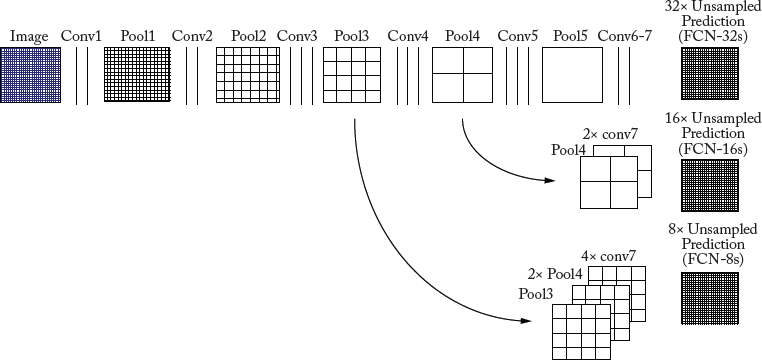
Figure 7.7: FCN learns to combine shallow layer (fine) and deep layer (coarse) information. The first row shows FCN-32s, which up-samples predictions back to pixels in a single step. The second row illustrates FCN-16s, which combines predictions from both the final and the pool4 layer. The third row shows FCN-8s, which provides further precision by considering additional predictions from pool3 layer.
FCN-8s
In order to obtain more accurate prediction maps, FCN-8s combines predictions from the final convolutional layer and shallower layers, i.e., pool3 and pool4 layers. The third row of Fig. 7.7 shows the architecture of the FCN-8s network. First, a 1 × 1 convolutional layer with channel dimension of 21 is added on top of pool3 layer to predict new scores at stride 8 for each of the PASCAL VOC classes. Then, the summed predicted scores at stride 16 (second row in Fig. 7.7) is passed through a transposed convolutional layer (i.e., 2× up-sampling layer) to produce new prediction scores at stride 8. These two predicted scores at stride 8 are summed up and then fed to another transposed convolutional layer (i.e., 8× up-sampling layer) to produce prediction maps with the same size as the input image. FCN-8s improved the performance of FCN-18s by a small mean IoU and achieved 62.7 mean IoU on the PASCAL VOC 2011.
FCN Fine-tuning
Since training from scratch is not feasible due to the large number of training parameters and the small number of training samples, fine-tuning using back-propagation through the entire network is done to train FCN for segmentation. It is important to note that FCN uses whole image training instead of patch-wise training, where the network is learned from batches of random patches (i.e., small image regions surrounding the objects of interest). Fine-tuning of the coarse FCN-32s version, takes three GPU days, and about one day on GPU each for the FCN-16s and FCN-8s [Long et al., 2015]. FCN has been tested on PASCAL VOC, NYUDv2, and SIFT Flow datasets for the task of segmentation. It has been shown to achieve superior performance compared to other reported methods.
FCN Drawbacks
FCN discussed above has few limitations. The first issue is related to a single transposed convolutional layer of FCN, which cannot accurately capture the detailed structures of objects. While FCN-16s and FCN-8s attempt to avoid this issue by combining coarse (deep layer) information with fine (shallower layers) information, the detailed structure of objects are still lost or smoothed in many cases. The second issue is related to the scale, i.e., fixed-size receptive field of FCN. This causes the objects that are larger or smaller than the receptive field to be mislabeled. To overcome these challenges, Deep Deconvolution Network (DDN) has been proposed, which is discussed in the following section.
7.3.2 DEEP DECONVOLUTION NETWORK (DDN)
DDN [Noh et al., 2015] consists of convolution (Module A shown in Fig. 7.8) and deconvolution networks (Module B). The convolution network acts as a feature extractor and converts the input image to a multi-dimensional feature representation. On the other hand, the deconvolution network is a shape generator, that uses these extracted feature maps and produces class score prediction maps at the output with a spatial size of the input image. These class score prediction maps represent the probability that each pixel belongs to different classes.
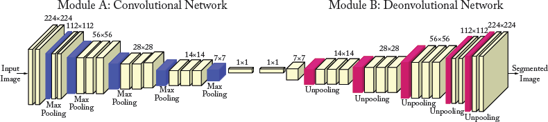
Figure 7.8: Overall architecture of deep deconvolution network. A multilayer deconvolution network is put on top of the convolution network to accurately perform image segmentation. Given a feature representation from the convolution network (Module A), dense class score prediction maps are constructed through multiple un-pooling and transposed convolution layers (Module B).
DDN uses convolutionalized VGGnet-16 network for the convolutional part. More precisely, the last fully connected layer of VGGnet-16 is removed and the last two fully connected layers are converted to convolutional layers (similar to FCN). The deconvolution part is the reciprocal of the convolution network. Unlike FCN-32s, which uses a single transposed convolutional layer, the deconvolution network of DDN uses a sequence of un-pooling and transposed convolution layers to generate class prediction maps with the same spatial size as the input image. In contrast to the convolution part of the model, which decreases the spatial size of the output feature maps through feed-forwarding, its counterpart increases the size by combining the transposed convolution and un-pooling layers.
Un-pooling Layer
The un-pooling layers of the deconvolution network of DDN perform the reverse operation of the max-pooling layers of the convolution network. To be able to perform reverse max-pooling, the max-pooling layers save the locations of the maximum activations in their “switch variables,” i.e., essentially the argmax of the max-pooling operation. The un-pooling layers then employ these switch variables to place the activations back to their original pooled locations.
DDN Training
To train this very deep network with relatively small training examples, the following strategies are adopted. First, every convolutional and transposed convolutional layer is followed by a batch normalization layer (discussed in Section 5.2.4), which has been found to be critical for DDN optimization. Second, unlike FCN which performs image-level segmentation, DDN uses instance-wise segmentation, in order to handle objects in various scales and decrease the training complexity. For this purpose, a two-stage training approach is used.
In the first phase, DDN is trained with easy samples. To generate the training samples for this phase, ground-truth bounding box annotations of objects are used to crop each object so that the object is centered at the cropped bounding box. In the subsequent phase, the learned model from the first phase is fine-tuned with more challenging samples. Thus, each object proposal contributes to the training samples. Specifically, the candidate object proposals, which sufficiently overlap with the ground-truth segmented regions (≥ 0.5 in IoU) are selected for training. To include context, post-processing is also adopted in this phase.
DDN Inference
Since DDN uses instance-wise segmentation, an algorithm is required to aggregate the output score prediction maps of individual object proposals within an image. DDN uses the pixel-wise maximum of the output prediction maps for this purpose. More precisely, the output prediction maps of each object proposal (gi ∈ RW×H×C, where C is the number of classes and i, W and H denote the index, height and width of the object proposal, respectively) are first superimposed on the image space with zero padding outside gi. Then, the pixel-wise prediction map of the entire image is computed as follows:
where Gi is the prediction map corresponding to gi in the image space with zero padding outside gi. Next, a soft-max loss is applied to the aggregated prediction maps, P in Eq. (7.4), to obtain class probability maps (O) in the entire image space. The final pixel-wise labeled image is computed by applying the fully connected CRF [Krähenbühl and Koltun, 2011] to the output class probability maps O.
Conditional Random Field (CRF): CRF is a class of statistical modeling technique, which are categorized as the sequential version of logistic regression. In contrast to logistic regression, which is a log linear classification model, CRFs are log linear models for sequential labeling.
The CRF is defined as the conditional probabilities of X and Y, represented as P(Y|X), where X denotes a multi-dimensional input, i.e., features, and Y denotes a multi-dimensional output, i.e., labels. The probabilities can be modeled in two different ways, i.e., unary potential and pairwise potential. Unary potential is used to model the probabilities that a given pixel or a patch belongs to each particular category, while pairwise potential is defined to model the relation between two different pixels and patches of an image. In fully connected CRF, e.g., Krähenbühl and Koltun [2011], the latter approach is explored to establish pairwise potential on all pixel pairs in a given image, thus resulting into refined segmentation and labeling. For more details on CRF, the readers are referred to Krähenbühl and Koltun [2011].
DDN Testing
For each testing image, approximately 2,000 object proposals are generated using edge-box algorithm [Zitnick and Dollár, 2014]. Next, the best 50 proposals with the highest objectness scores are selected. These object proposals are then used to compute instance-wise segmentations, which are then aggregated, using the algorithm discussed above, to obtain the semantic segmentation for the whole image. DDN has been shown to achieve an outstanding performance of 72.5% on PASCAL VOC 2012 dataset compared to other reported methods.
DDN Drawbacks
DDN discussed above has a couple of limitations. First, DDN uses multiple transposed convolutional layers in its architecture, which requires additional memory and time. Second, training DDN is tricky and requires a large corpus of training data to learn the transposed convolutional layers. Third, DDN deals with objects at multiple scales by performing instant-wise segmentation. Therefore, it requires feed-forwarding all object proposals through the DDN, which is a time-consuming process. To overcome these challenges, DeepLab model has been proposed, which is discussed in the following section.
In DeepLab [Chen et al., 2014], the task of semantic segmentation has been addressed by employing convolutional layers with up-sampled filters, which are called atrous convolution (or dilated convolution as discussed in Chapter4).
Recall that forward passing an input image through the typical convolution classification networks reduces the spatial scale of the output feature maps, typically by a factor of 32. However, for dense predictions tasks, e.g., semantic segmentation, a stride of 32 pixels limits the level of details in the up-sampled output maps. One partial solution is to append multiple transposed convolutional layers as in FCN-8s and DDN, to the top of the convolutionalized classification networks to produce output maps with the same size of the input image. However, this approach is too costly.5 Another critical limitation of these convolutionalized classification networks is that they have a predefined fixed-size receptive field. For example, FCN and all its variants (i.e., FCN-16s and FCN-8s) use VGNNnet-16 with fixed-size 3 × 3 filters. Therefore, an object with a substantially smaller or larger spatial size than the receptive field is problematic.6
DeepLab uses atrous convolution in its architecture to simultaneously address these two issues. As discussed in Chapter 4, atrous convolution allows to explicitly control the spatial size of the output feature maps that are computed within convolution networks. It also extends the receptive field, without increasing the number of parameters. Thus, it can effectively incorporate a wider image context while performing convolutions. For example, to increase the spatial size of the output feature maps in the convolutionalized VGGnet-16 network7 by a factor of 2, one could set the stride of the last max-pooling layer (pool5) to 1, and then substitute the subsequent convolutional layer (conv6, which is the convolutionalized version of fc6) with the atrous convolutional layers with a sampling factor d = 2. This modification also extends the filter size of 3 × 3 to 5 × 5, and therefore enlarges the receptive field of the filters.
DeepLab-LargeFOV Architecture
DeepLab-LargeFOV is a CNN with an atrous convolutional layer which has a large receptive field. Specifically, DeepLab-LargeFOV is built by converting the first two fully-connected layers of VGGnet-16 (i.e., fc6 and fc7) to convolutional layers (i.e., conv6 and conv7) and then appending a 1 × 1 convolution layer (i.e., conv8) with 21 channels at the end of the convolutionalized networks for semantic segmentation on PASCAL VOC dataset. The stride of the last two max-pooling layers (i.e., pool4 and pool5) is changed to 1,8 and the convolutional filter of conv6 layer is replaced with an atrous convolution of kernel size 3 × 3 and an atrous sampling factor d = 12. Therefore, the spatial size of the output class score prediction maps is increased by a factor of 4. Finally, a fast bilinear interpolation layer9 (i.e., 8× up-sampling) is employed to recover the output prediction maps at the original image size.
Atrous Spatial Pyramid Pooling (ASPP)
In order to capture objects and context at multiple scales, DeepLab employs multiple parallel atrous convolutional layers (discussed in Section 4.2.2) with different sampling factors d, which is inspired by the success of the Spatial Pyramid Pooling (SPP) layer discussed in Section 4.2.8. Specifically, DeepLab with atrous Spatial Pyramid Pooling layer (called DeepLab-ASPP) is built by employing 4 parallel conv6 – conv7 – conv8 branches with 3 × 3 filters and different atrous factors (d = {6, 12, 18, 24}) in the conv6 layers, as shown in Fig. 7.9. The output prediction maps from all four parallel branches are aggregated to generate the final class score maps. Next, a fast bilinear interpolation layer is employed to recover the output prediction maps with the original image size.

Figure 7.9: Architecture of DeepLab-ASPP (DeepLab with Atrous Spatial Pyramid Pooling layer). pool5 denotes the output of the last pooling layer of VGGnet-16.
DeepLab Inference and Training
The output prediction maps of the bilinear interpolation layer can only predict the presence and rough position of objects, but the boundaries of objects cannot be recovered. DeepLab handles this issue by combining the fully connected CRF [Krähenbühl and Koltun, 2011] with the output class prediction maps of the bilinear interpolation layer. The same approach is also used in DDN. During training, the Deep Convolutional Neural Network (DCNN) and the CRF training stages are decoupled. Specifically, a cross validation of the fully connected CRF is performed after the fine-tuning of the convolutionalized VGGnet-16 network.
DeepLab Testing
DeepLab has been tested on the PASCAL VOC 2012 validation set and has been shown to achieve state-of-the-art performance of 71.6% mean IoU compared to other reported methods including fully convolutional networks. Moreover, DeepLab with atrous Spatial Pyramid Pooling layer (DeepLab-ASPP) achieved about 2% higher accuracy than DeepLab-LargeFOV. Experimental results show that DeepLab based on ResNet-101 delivers better segmentation results compared to Deep Lab employing VGGnet-16.
In computer vision, the recognition of single or isolated objects in a scene has achieved significant success. However, developing a higher level of visual scene understanding requires more complex reasoning about individual objects, their 3D layout and mutual relationships [Khan, 2016, Li et al., 2009]. In this section, we will discuss how CNNs have been used in the area of scene understanding.
DeepContext [Zhang et al., 2016] presents an approach to embed 3D context into the topology of a neural network, trained to perform holistic scene understanding. Given an input RGB-D image, the network can simultaneously make global predictions (e.g., scene category and 3D scene layout) as well as local decisions (e.g., the position and category of each constituent object in the 3D space). This method works by first learning a set of scene templates from the training data, which encodes the possible locations of single or multiple instances of objects belonging to a specific category. Four different scene templates, including sleeping area, lounging area, office area, and a table and chair sets are used. Given this contextual scene representation, DeepContext matches an input volumetric representation of an RGBD image with one of the scene templates using a CNN (Module B, Fig. 7.10). Afterward, the input scene is aligned with the scene template using a transformation network (Module C, Fig. 7.10). The aligned volumetric input is fed to a deep CNN with two main branches; one works on the complete 3D input and obtains a global feature representation while the second works on the local object level and predicts the location and existence of each potential object in the aligned template (Module D, Fig. 7.10).

Figure 7.10: The block diagram for DeepContext processing pipeline. Given a 3D volumetric input (module A), the transformation network (module C) aligns the input data with its corresponding scene template (estimated by module B). Using this roughly aligned scene, the 3D context network (module D) estimates the existence of an object and adjusts the object location based on local object features and holistic scene features, to understand a 3D scene.
The DeepContext algorithm follows a hierarchical process for scene understanding which is discussed below.
Learning Scene Templates
The layouts of the scene templates (e.g., office, sleeping area) are learned from the SUN RGB-D dataset [Song et al., 2015], which comes with 3D object bounding box annotations. Each template represents a scene context by summarizing the bounding box locations and the category information of the objects that are present in the training set. As an initial step, all the clean examples of each scene template (i.e., sleeping area, lounging area, office area and a table and chair sets) are identified. Next, a major object is manually identified in each scene template (e.g., a bed in the sleeping area) and its position is used to align all the scenes belonging to a specific category. This rough alignment is used to find the most frequent locations for each object (also called “anchor positions”) by performing k-means clustering and choosing the top k centers for each object. Note that the object set includes not only the regular objects (e.g., bed, desk) but also the scene elements which define the room layout (e.g., walls, floor and ceiling).
The clean dataset of the scene categories used to learn the scene templates, is also used in subsequent processing stages, such as scene classification, scene alignment, and 3D object detection. We will discuss these stages below.
Scene Classification (Module B, Fig. 7.10)
A global CNN is trained to classify an input image to one of the scene templates. Its architecture is exactly same as the global scene pathway in Fig. 7.11. Note that the input to the network is a 3D volumetric representation of the input RGB-D images, which is obtained using the Truncated Signed Distance Function (TSDF) [Song and Xiao, 2016]. This first representation is processed using three processing blocks, each consisting of a 3D convolution layer, a 3D pooling layer, and a ReLU nonlinearity. The output is an intermediate “spatial feature” representation corresponding to a grid of 3D spatial locations in the input. It is further processed by two fully connected layers to obtain a “global feature” which is used to predict the scene category. Note that both the local spatial feature and the global scene-level feature is later used in the 3D context network.
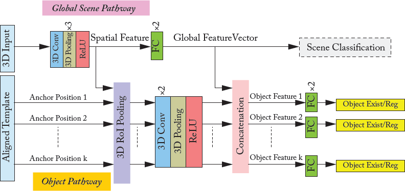
Figure 7.11: Deep 3D Context network (Module D, Fig. 7.10) architecture. The network consists of two channels for global scene-level recognition and local object-level detection. The scene pathway is supervised with the scene classification task during pre-training only (Module B). The object pathway performs object detection, i.e., predicts the existence/non-existence of an object and regresses its location. Note that the object pathway brings in both local and global features from the scene pathway.
3D Transformation Network (Module C, Fig. 7.10)
Once the corresponding scene template category has been identified, a 3D transformation network estimates a global transformation which aligns the input scene to the corresponding scene-template. The transformation is calculated in two steps: a rotation followed by a translation. Both these transformation steps are implemented individually as classification problems, for which CNNs are well suited.
For the rotation, only the rotation about the vertical-axis (yaw) is predicted since the gravity direction is known for each scene in the SUN RGB-D dataset. Since an exact estimation of the rotation along the vertical axis is not required, the 360° angular range is divided into 36 regions, each encompassing 10°. A 3D CNN is trained to predict the angle of rotation along the vertical axis. The CNN has the same architecture as the one used in Module B (scene classification), however, its output layer has 36 units which predicts one of the 36 regions denoting the y-axis rotation.
Once the rotation has been applied, another 3D CNN is used to estimate the translation that is required to align the major object (e.g., bed, desk) in the input scene and the identified scene template. Again, the CNN has essentially the same architecture as Module B, however, the last layer is replaced by a soft-max layer with 726 units. Each value of the output units denotes a translation in a discretized space of 11 × 11 × 6 values. Similar to rotation, the estimated translation is also a rough match due to the discretized set of values. Note that for such problems (i.e., parameter estimation), regression is a natural choice since it avoids errors due to discretization. However, the authors could not successfully train a CNN with a regression loss for this problem. Since the context network regresses the locations of each detected object in the scenes in the next stage, a rough alignment suffices at this stage. We explain the context network below.
3D Context Network (Fig. 7.11)
The context neural network performs 3D object detection and layout estimation. A separate network is trained for each scene template category. This network has two main branches, as shown in Fig. 7.11: a global scene level branch and a local object level branch. Both network pathways encode different levels of details about the 3D scene input, which are complementary in nature. The local object-level branch is dependent on the features from the initial and final layers of the global scene-level branch. To avoid any optimization problems, the global scene-level branch is initialized with the weights of the converged scene classification network (Module B) (since both have the same architecture). Each category-specific context network is then trained separately using only the data from that specific scene template. During this training procedure, the scene-level branch is fine-tuned while the object-level branch is trained from scratch.
The object-level branch operates on the spatial feature from the global scene-level branch. The spatial feature is the output activation map after the initial set of three processing layers, each consisting of a 3D convolution, pooling, and ReLU layers. This feature map is used to calculate object-level features (corresponding to anchor positions) at a 6 × 6 × 6 resolution using the 3D Region of Interest (RoI) pooling. The 3D RoI pooling is identical to its 2D counterpart described in Section 4.2.7, with only an extra depth dimension. The pooled feature is then processed through 3D convolution and fully connected layers to predict the object existence and its location (3D bounding box). The object location is regressed using the R-CNN localization loss to minimize the offset between the ground-truth and the predicted bounding boxes (Section 7.2.1).
Hybrid Data for Pre-training
Due to the lack of huge amount of RGB-D training data for scene understanding, this approach uses an augmented dataset for training. In contrast to the simple data augmentation approaches we discussed in Section 5.2.1, the proposed approach is more involved. Specifically, a hybrid training set is generated by replacing the annotated objects from the SUN RGB-D dataset with the same category CAD models. The resulting hybrid set is 1,000 times bigger than the original RGBD training set. For the training of 3D context network (scene pathway), the models are trained on this large hybrid dataset first, followed by a fine-tuning on the real RGB-D depth maps to ensure that the training converges. For the alignment network, the pre-trained scene pathway from the 3D context network is used for the initialization. Therefore, the alignment network also benefits from the hybrid data.
The DeepContext model has been evaluated on the SUN RGB-D dataset and has been shown to model scene contexts adequately.
7.4.2 LEARNING RICH FEATURES FROM RGB-D IMAGES
The object and scene level reasoning system presented in the previous section was trained end-to-end on 3D images. Here, we present an RGB-D- (2.5D instead of 3D) based approach [Gupta et al., 2014] which performs object detection, object instance segmentation, and semantic segmentation, as shown in Fig. 7.12. This approach is not end-to-end trainable, it rather extends the pre-trained CNN on color images to depth images by introducing a new depth encoding method. This framework is interesting, since it demonstrates how pre-trained networks can be effectively used to transfer learning from domains where large quantities of data is available to the ones where labeled data is scarce, and even for new data modalities (e.g., depth in this case). In the following sections, we briefly discuss the processing pipeline (summarized in Fig. 7.12).
Encoding Depth Images for Feature Learning
Instead of directly training a CNN on the depth images, Gupta et al. [2014] propose to encode the depth information using three geometric features calculated at each pixel location. These include: the horizontal disparity, the height above the ground, and the angle between the surface normals at a given pixel and the estimated gravity direction. This encoding is termed as the HHA encoding (first letter of each geometric feature). For the training dataset, all these channels are mapped to a constant range of 0–255.
The HHA encoding and color images are then fed to the deep network to learn more discriminative feature representations on top of the geometric features based on raw depth information. Since the NYU-Depth dataset used in this work, consisted of only 400 images, an explicit encoding of the geometric properties of the data made a big difference to the network, which usually requires much larger amounts of data to automatically learn the best feature representations. Furthermore, the training dataset was extended by rendering synthetic CAD models in the NYU-Depth dataset scenes. This is consistent with the data augmentation approach that we discussed for the case of DeepContext [Zhang et al., 2016].
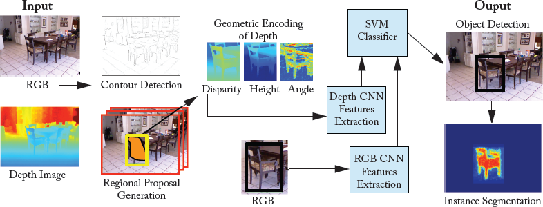
Figure 7.12: The input to this framework is a RGB and a depth image. First, object proposals are generated using the contour information. The color and the encoded depth image are passed through separately trained CNNs to obtain features which are then classified into object categories using the SVM classifiers. After detection, a Random Forest classifier is used to identify foreground object segmentation within each valid detection.
CNN Fine-tuning for Feature Learning
Since the main goal of this work is object detection, it is useful to work on the object proposals. The region proposals are obtained using an improved version of Multiscale Combinatorial Grouping (MCG) [Arbeláez et al., 2014] approach which incorporated additional geometric features based on the depth information. The regions proposals which have a high overlap with the ground-truth object bounding box are first used to train a deep CNN model for classification. Similar to R-CNN, the pre-trained AlexNet [Krizhevsky et al., 2012] is fine-tuned for this object classification task. Once the network is fine-tuned, object specific linear classifiers (SVMs) are trained using the intermediate CNN features for the object detection task.
Instance Segmentation
Once the object detections are available, the pixels belonging to each object instance are labeled. This problem is tackled by predicting the foreground or background label for each pixel within a valid detection. For this purpose, a random forest classifier is used to provide the pixel level labelings. This classifier is trained on the local hand-crafted features whose details are available in Gupta et al. [2013]. Since these predictions are calculated roughly for individual pixels, they can be noisy. To smooth the initial predictions of the random forest classifier, these predictions are averaged on each super-pixel. Note that subsequent works on instance segmentation (e.g., He et al. [2017]) have incorporated a similar pipeline (i.e., first detecting object bounding boxes and then predicting the foreground mask to label the individual object instance). However, in contrast to Gupta et al. [2014], He et al. [2017] use an end to end trainable CNN model which avoids manual parameter selection and a series of isolated processing steps toward the final goal. As a result, He et al. [2017] achieve highly accurate segmentations compared to the non-end-to-end trainable approaches.
Another limitation of this approach is the separate processing of both color and depth images. As we discussed in Chapter 6, AlexNet has a huge number of parameters, and learning two separate set of parameters for both modalities doubles the parameter space. Moreover, since both images belong to the same scene, we expect to learn better cross-modality relationships if both modalities are considered jointly. One approach to learn a shared set of parameters in such cases is to stack the two modalities in the form of a multichannel input (e.g., six channels) and perform a joint training over both modalities [Khan et al., 2017c, Zagoruyko and Komodakis, 2015].
7.4.3 POINTNET FOR SCENE UNDERSTANDING
PointNet (discussed in Section 7.1.1) has also been used for scene understanding by assigning a semantically meaningful category label to each pixel in an image (Module B in Figure 7.1). While we have discussed the details of PointNet before, it is interesting to note its similarity with the Context Network in DeepContext (Section 7.4.1 and Figure 7.11). Both these networks learn an initial representation, shared among the global (scene classification) and the local (semantic segmentation or object detection) tasks. Afterward, the global and local branches split up, and the scene context is added in the local branch by copying the high-level features from the global branch to the local one. One can notice that the incorporation of both the global and local contexts are essential for a successful semantic labeling scheme. Other recent works in scene segmentation are also built on similar ideas, i.e., better integration of scene context using for example a pyramid-based feature description [Zhao et al., 2017], dilated convolutions [Yu and Koltun, 2015], or a CRF model [Khan et al., 2016a, Zheng et al., 2015].
Recent advances in image modeling with neural networks, such as Generative Adversarial Networks (GANs) [Goodfellow et al., 2014], have made it feasible to generate photo-realistic images, which can capture the high-level structure of the natural training data [van den Oord et al., 2016]. GANs are one type of generative networks, which can learn to produce realistic-looking images in an unsupervised manner. In recent years, a number of GAN-based image generation methods have emerged which work quite well. One such promising approach is Deep Convolutional Generative Adversarial Networks (DCGANs) [Radford et al., 2015], which generates photo-realistic images by passing random noise through a deep convolutional network. Another interesting approach is Super-Resolution Generative Adversarial Networks (SRGAN) [Ledig et al., 2016], which generates high-resolution images from low-resolution counterparts. In this section, we shall first briefly discuss GANs and then extend our discussion to DCGANs and SRGAN.
7.5.1 GENERATIVE ADVERSARIAL NETWORKS (GANS)
GANs were first introduced by Goodfellow et al. [2014]. The main idea behind a GAN is to have two competing neural network models (shown in Fig. 7.13). The first model is called generator, which takes noise as input and generates samples. The other neural network, called discriminator, receives samples from both the generator (i.e., fake data) and the training data (i.e., real data), and discriminates between the two sources. These two networks undergo a continuous learning process, where the generator learns to produce more realistic samples, and the discriminator learns to get better at distinguishing generated data from real data. These two networks are trained simultaneously with the aim that this training will drive the generated samples to be indistinguishable from real data. One of the advantages of GANs is that they can back-propagate the gradient information from the discriminator back to the generator network. The generator, therefore, knows how to adapt its parameters in order to produce output data that can fool the discriminator.

Figure 7.13: Generative Adversarial Networks Overview. Generator takes the noise as an input and generates samples. The discriminator distinguishes between the generator samples and the training data.
GANs Taining
The training of GANs involves the computation of two loss functions, one for the generator and one for the discriminator. The loss function for the generator ensures that it produces better data samples, while the loss function for the discriminator ensures that it distinguishes between the generated and real samples. We now briefly discuss these loss functions. For more details, the readers are referred to Goodfellow [2016].
The discriminator’s loss function J(D) is represented by:

which is the cross entropy loss function. In this equation, θ(D) and θ(G) are the parameters of the discriminator and the generator networks, respectively. pdata denotes the distribution of real data, x is a sample from pdata, p(z) is the distribution of the generator, z is a sample from P(z), G(z) is the generator network and D is the discriminator network. One can note from Eq. (7.5) that the discriminator is trained as a binary classifier (with sigmoid output) on two mini-batches of data. One of the them is from the data set containing real data samples with label 1 assigned to all examples, and the other from the generator (i.e., fake data) with label 0 for all the examples.
Cross-entropy: The cross-entropy loss function for the binary classification task is defined as follows:
where x1 and y1 ∈ [–1 1] denote a sample from a probability distribution function D and its desired output, respectively. After summing over m data samples, Eq. (7.5) can be written as follows:

In the case of GANs, data samples come from two sources, the discriminator’s distribution xi ~ pdata or the generator’s distribution xi = G(z), where z ~ P(z). Let’s assume that the number of samples from both distributions is equal. By writing Eq. (7.7) probabilistically, i.e., replacing the sums with expectations, the label yi with ![]() (because the number of samples from both generator and discriminator distributions is equal), and the log(1 − D(xi)) with log(1 − D(G(z))), we get the same loss function as Eq. (7.5), for the discriminator.
(because the number of samples from both generator and discriminator distributions is equal), and the log(1 − D(xi)) with log(1 − D(G(z))), we get the same loss function as Eq. (7.5), for the discriminator.
Generator Loss Function
The discriminator, discussed above, distinguishes between the two classes, i.e., the real and the fake data, and therefore needs the cross entropy function, which is the best option for such tasks. However, in the case of the generator, the following three types of loss functions can be used.
• The minimax Loss function: The minimax loss10 is the simplest version of the loss function, which is represented as follows:

The minimax version has been found to be less useful due to the gradient saturation problem. The latter occurs due to the poor design of the generator’s loss function. Specifically, as shown in Fig. 7.14, when the generator samples are successfully rejected by the discriminator with high confidence11 (i.e., D(G(z)) is close to zero), the generator’s gradient vanishes and thus, the generator’s network cannot learn anything.
• Heuristic, non-saturation loss function: The heuristic version is represented as follows:

This version of the loss function is based on the concept that the gradient of the generator is only dependent on the second term in Eq. (7.5). Therefore, as opposed to the minimax function, where the signs of J(D) are changed, in this case the target is changed, i.e., log D(G(z)) is used instead of log(1 − D(G(z))). The advantage of this strategy is that the generator gets a strong gradient signal at the start of the training process (as shown in Fig. 7.14), which helps it in attaining a fast improvement to generate better data, e.g., images.
• Maximum Likelihood loss function: As the name indicates, this version of the loss function is motivated by the concept of maximum likelihood (a well-known approach in machine learning) and can be written as follows:

where σ is the logistic sigmoid function. Like the minimax loss function, the maximum likelihood loss also suffers from the gradient vanishing problem when D(G(z)) is close to zero, as shown in Fig. 7.14. Moreover, unlike the minimax and the heuristic loss functions, the maximum likelihood loss, as a function of D(G(z)), has a very high variance, which is problematic. This is because most of the gradient comes from a very small number of the generator’s samples that are most likely to be real rather than fake.
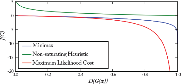
Figure 7.14: The loss response curves as functions of D(G(z)) for three different variants of the GAN generator’s loss functions.
To summarize, one can note that all three generator loss functions do not depend on the real data (x in Eq. (7.5)). This is advantageous, because the generator cannot copy input data x, which helps in avoiding the over-fitting problem in the generator. With this brief overview of generative adversarial models and their loss functions, we will now summarize the different steps that are involved in GANs training.
1. sampling a mini-batch of m samples from the real dataset pdata;
2. sampling a mini-batch of m samples from the generator p(z) (i.e., fake samples);
3. learning the discriminator by minimizing its loss function in Eq. (7.5);
4. sampling a mini-batch of m samples from the generator p(z)) (i.e., fake sample); and
5. learning the generator by minimizing its loss function in Eq. (7.9).
These steps are repeated until convergence occurs or until the iteration is terminated. With this brief overview of generative adversarial networks, we will now discuss two representative applications of GANs, known as DCGANs [Radford et al., 2015] and SRGAN [Ledig et al., 2016].
7.5.2 DEEP CONVOLUTIONAL GENERATIVE ADVERSARIAL NETWORKS (DCGANS)
DCGANs [Radford et al., 2015] are the first GAN models, which can generate realistic images from random input samples. In the following, we shall discuss the architecture and the training of DCGANs.
DCGANs provide a family of CNN architectures, which can be used in the generator and the discriminator parts of GANs. The overall architecture is the same as the baseline GAN architecture, which is shown in Fig. 7.13. However, the architecture of both the generator (shown in Fig. 7.15) and the discriminator (shown in Fig. 7.16) is borrowed from the all-convolutional network [Springenberg, 2015], meaning that these models do not contain any pooling or un-pooling layers. In addition, the generator uses transposed convolution to increase the representation’s spatial size, as illustrated in Fig. 7.15. Unlike the generator, the discriminator uses convolution to squeeze the representation’s spatial size for the classification task (Fig. 7.16). For both networks, a stride greater than 1 (usually 2) is used in the convolutional and transposed convolutional layers. Batch normalization is used in all layers of both the discriminator and the generator models of DCGANs with the exception of the first layer of the discriminator and the last layer of the generator. This is done to ensure that DGCAN learns the correct scale of the data distribution and its mean. DCGANs use the ReLU activation in all transposed convolutional layers except the output layer, which uses tanh activation function. It is because a bounded activation function such as tanh, allows the generator to speed-up the learning process and cover the color space of the samples from the training distribution. For the discriminator model, leaky ReLU (discussed in Section 4.2.4) was found to be better than ReLU. DCGANs use the Adam optimizer (discussed in Section 5.4.6) rather than SGD with momentum.
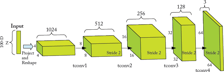
Figure 7.15: Example DCGAN generator’s architecture for Large-scale Scene Understanding (LSUN) dataset [Song and Xiao, 2015]. A 100-dimensional uniform distribution z is projected and then reshaped to a 4 × 4× 1,024 tensor, where 1,024 is the number of feature maps. Next, the tensor is passed through a sequence of transposed convolutional layers (i.e., tconv1 − tconv2 − tconv3 − tconv4) to generate a 64 × 64 × 3 realistic image.
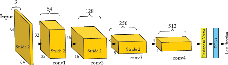
Figure 7.16: Example DCGAN discriminator’s architecture for LSUN dataset [Song and Xiao, 2015]. An 64 × 64 RGB input image is passed through a sequence of convolutional layers (i.e., conv1 − conv2 − conv3 − conv4) followed by a fully-connected layer with 2 outputs.
DCGANs as a Feature Extractor
DCGANs uses ImageNet as a dataset of natural images for unsupervised training to evaluate the quality of the features learned by DCGAN. For this purpose, DCGANs is first trained on ImageNet dataset. Note that the image labels are not required during training (unsupervised learning). Also, it is important to note that all the training and test images are scaled to the range of [-1, 1], i.e., the range of tanh activation function. No other pre-processing is done. Then, for each training image in a supervised dataset (e.g., CIFAR-10 dataset), the output feature maps from all the convolutional layers of the discriminator are max-pooled to produce a 4 × 4 spatial grid for each layer. These spatial grids are then flattened and concatenated to form a high dimensional feature representation of the image. Finally, an ℓ2 regularized linear SVM is trained on the high dimensional feature representation of all the training images in the supervised dataset. It is interesting to note that although DCGAN is not trained on the supervised dataset, it outperforms all K-means-based methods. DCGANs can also be used for image generation. For example, experiments show that the output of the last layer in the generator network of DCGAN trained on LSUN dataset [Song and Xiao, 2015] produces really cool bedroom images.
7.5.3 SUPER RESOLUTION GENERATIVE ADVERSARIAL NETWORK (SRGAN)
In Ledig et al. [2016], a generative adversarial network for single SRGAN is presented, where the input to the network is a low-resolution (LR) image and the output is its high-resolution (HR) counterpart. Unlike existing optimization-based super resolution techniques, which rely on the minimization of the Mean Squared Error (MSE) as loss function, this technique proposes the perceptual loss function for the generator. The latter is comprised of two losses which are called “content loss” and “adversarial loss.” In the following, we will briefly discuss these loss functions, followed by the architecture of SRGAN.
Content Loss
The MSE loss function smooths images by suppressing the high-frequency contents, which results in perceptually unsatisfied solutions [Ledig et al., 2016]. To overcome this problem, a content loss function that is motivated by perceptual similarity is used in SRGAN:

where ILR and IHR are the LR and HR images, ϕ(·) is the output feature map produced by a convolutional layer of VGGnet-19, W and H are the width and the height of the feature map, respectively. In summary, Eq. (7.11) computes the Euclidean distance between the output feature maps (i.e., the output of a convolutional layer of the pre-trained VGGnet-19) of the generated image ![]() and the real high resolution image IHR. Note that the pre-trained VGGnet-19 is only used as a feature extractor (i.e., its weight parameters are not changed during the training of SRGAN).
and the real high resolution image IHR. Note that the pre-trained VGGnet-19 is only used as a feature extractor (i.e., its weight parameters are not changed during the training of SRGAN).
Adversarial Loss
The adversarial loss is the same as the heuristic loss function in the baseline GAN (Eq. (7.9)), and is defined as follows:
where ![]() is the probability that the image produced by the generator,
is the probability that the image produced by the generator, ![]() , is a HR image (i.e., real image).
, is a HR image (i.e., real image).
Perceptual Loss Function as the Generator Loss
The perceptual loss function, which is used as the generator loss in SRGAN, is calculated as the weighted sum of the content loss and the adversarial loss, discussed above and is given by:
where![]() represents the content loss, while
represents the content loss, while ![]() is the adversarial loss.
is the adversarial loss.
Discriminator Loss
The discriminator loss is the cross-entropy loss function (Eq. (7.5)), which is trained as a binary classifier (HR or LR class) with a sigmoid output.
Similar to the baseline GAN [Goodfellow et al., 2014], SRGAN has two key components: the discriminator and the generator. We will now briefly discuss the architecture of these two SRGAN components.
Discriminator Network of SRGAN
The discriminator network of SRGAN, shown in Fig. 7.17, is inspired by the architecture of DCGAN (discussed in Section 7.5.2). The network consists of eight convolutional layers with 3 × 3 convolution kernels followed by two fully connected layers, and a sigmoid function to perform binary classification.

Figure 7.17: Architecture of the discriminator network of SRGAN. k, n, and s represent the kernel size, number of feature maps, and stride for each convolutional layer.
Generator Network of SRGAN
The generator component of the SRGAN, shown in Fig. 7.18, is inspired by the deep residual network (discussed in Section 6.6) and the architecture of DCGAN (discussed in Section 7.5.2). As suggested by DCGAN [Radford et al., 2015], a leaky ReLU activation function is used in all layers. Moreover, batch normalization is used after all convolutional layers with the exception of the first convolutional layer.

Figure 7.18: Architecture of the generator network of SRGAN. Similar to the discriminator network, k, n, and s represent the kernel size, number of feature maps, and stride for each convolutional layer.
In summary, SRGAN is able to estimate high resolution images with photo-realistic textures from heavily down-sampled images. It achieved a very good performance on three publicly available datasets including Set5, Set14, and BSD100.
7.6 VIDEO-BASED ACTION RECOGNITION
Human action recognition in videos is a challenging research problem, which has received a significant amount of attention in the computer vision community [Donahue et al., 2015, Karpathy et al., 2014, Rahmani and Bennamoun, 2017, Rahmani and Mian, 2016, Rahmani et al., 2017, Simonyan and Zisserman, 2014a]. Action recognition aims to enable computers to automatically recognize human actions from real world videos. Compared to the single-image classification, the temporal extent of action videos provides an additional information for action recognition. Inspired by this, several approaches have been proposed to extend state-of-the-art image classification CNNs (e.g., VGGnet, ResNet) for action recognition from video data. In this section, we shall briefly discuss three representative CNN-based architectures used for video-based human action recognition task.
7.6.1 ACTION RECOGNITION FROM STILL VIDEO FRAMES
CNNs have so far achieved promising image recognition results. Inspired by this, an extensive evaluation of CNNs for extending the connectivity of a CNN to the temporal domain for the task of large-scale action recognition is provided in Karpathy et al. [2014]. We shall now discuss different architectures for encoding temporal variations of action videos.
Single Frame Architecture
We discuss a single-frame baseline architecture, shown in Fig. 7.19a, to analyze the contribution of the static appearance to the classification accuracy. The single frame model is similar to the AlexNet [Krizhevsky et al., 2012], which won the ImageNet challenge. However, instead of accepting the original input of size 224 × 224 × 3, the network takes 170 × 170 × 3 sized image. This network has the following configuration: Covn(96, 11, 3) – N – P – Conv(256, 5, 1) – N – P – Conv(384, 3, 1) – Conv(384, 3, 1) – Conv(256, 3, 1) – P – FC(4096) – FC(4096), where Conv(f, s, t) represents a convolutional layer, which has filters f of spatial size s × s and an input stride t. A fully connected layer, with n nodes, is represented by FC(n). For the pooling layers P and all the normalization layers N the architectural details described in Krizhevsky et al. [2012] are used along with the following parameters: k = 2; n = 5; α = 10–4; β = 0.5, where the constants k, n, α, and β are hyper-parameters. A softmax layer is connected to the last fully connected layer with dense connections.
Given an entire action video, the video-level prediction is produced by forward propagating each frame individually through the network and then averaging individual frame predictions over the durations of the video.

Figure 7.19: Approaches for fusing information over the temporal dimension through the network. (a) Single Frame, (b) Early Fusion, (c) Late Fusion, and (d) Slow Fusion. In the Slow Fusion Model (d), the depicted columns share parameters. The pink, green, and blue boxes denote convolutional, normalization and pooling layers, respectively.
Early Fusion Architecture
We now discuss the Early Fusion model (Fig. 7.19b). This model captures an entire time window information and combines it across at a pixel level. To achieve this, the filters on the first Conv layer in the single frame network (described above) are modified. The new filters have a size of 11 × 11 × 3 × T pixels, where T defines the temporal extent and is set to 10. This direct and early connectivity to the pixel data helps this model to accurately detect the speed and the direction of the local motion.
For a given entire video, 20 randomly selected sample clips are individually passed through the network and their class predictions are then averaged to produce video-level action class prediction.
Late Fusion Architecture
The late fusion model (Fig. 7.19c) consists of two separate single frame networks (described above) with shared parameters up to the last Conv layer, Conv(256, 3, 1). The outputs of the last Conv layer of these two separate single frame networks are then merged in the first fully connected layer. Global motion characteristics are computed by the first fully connected layer by comparing the output of both single-frame networks. These two separate single frame networks are placed at a distance of 15 frames apart. More precisely, the input to the first and the second single frame networks is the i-th frame and i + 15-th frame, respectively.
This model (Fig. 7.19d) slowly fuses the temporal information throughout the network in such way that the higher layers have access to more global information in both the temporal and the spatial domains. This is achieved by performing a temporal convolution along with a spatial convolution to calculate the weights and by extending the connectivity of all convolutional layers in time. More precisely, as shown in Fig. 7.19d, every filter in the first convolutional layer is applied on an input clip, with a size of 10 frames. The temporal extent of each filter is T = 4 and the stride is equal to 2. Thus, 4 responses are produced for each video clip. This process is iterated by the second and third layers with filters of temporal extent T = 2 and a stride equal to 2. Therefore, the information across all the input frames (a total of 10) can be accessed by the third convolutional layer.
Given an entire human action video, video-level classification is performed by passing 20 randomly selected sample clips through the network and then averaging individual clip predictions over the durations of the video.
Multi-resolution Architecture
In order to speed-up the above mentioned models while retaining their accuracy, the multiresolution architecture has been proposed in Karpathy et al. [2014]. The multi-resolution model consists of two separate networks (i.e., fovea and context networks) over two spatial resolutions, as shown in Fig 7.20. The architecture of the fovea and context networks is similar to the single-frame architecture discussed above. However, instead of accepting the original input of size 170 × 170 × 3, these networks take 89 × 89 × 3 sized images. More precisely, the input to the fovea model is the center region of size 89 × 89 at the original spatial resolution, while for the context stream the down-sampled frames at half the original resolution are used. The total dimensionality of the inputs is therefore halved. Moreover, the last pooling layer is removed from both the fovea and context networks and the activation outputs of both networks are concatenated and fed into the first fully connected layer.
Model Comparison
All models were trained on the Sport-1M dataset [Simonyan and Zisserman, 2014a], which consists of 200,000 test videos. The results showed that the variation among different CNN architectures (e.g., Single Frame, Multi-resolution, Early, Late, and Slow Fusion) is surprisingly insignificant. Moreover, the results were significantly worse than the state-of-the-art handcrafted shallow models. One reason is that these models cannot capture the motion information in many cases. For example, the Slow Fusion model is expected to implicitly learn the spatiotemporal features in its first layers, which is a difficult task [Simonyan and Zisserman, 2014a]. To resolve this issue, two-stream CNNs [Simonyan and Zisserman, 2014a] model was proposed to explicitly take into account both spatial and temporal information in a single end-to-end learning framework.

Figure 7.20: Multi-resolution architecture. Input frames are passed through two separate streams: a context stream which models the low-resolution image and a fovea stream which processes the high-resolution center crop image. The pink, green, and blue boxes denote convolutional, normalization, and pooling layers, respectively. Both streams converge to two fully connected layers (yellow boxes).
The two-stream CNNs model [Simonyan and Zisserman, 2014a] (shown in Fig. 7.21) uses two separate spatial and temporal CNNs, which are then combined by late fusion. The spatial network performs action recognition from single video frames, while the temporal network is learned to recognize action from motion, i.e., dense optical flow. The idea behind this two-stream model is related to the fact that the human visual cortex contains two pathways for object and motion recognition, i.e., the ventral stream performs object recognition and the dorsal stream recognizes motion.
Spatial Stream CNN
The spatial stream CNN model is similar to the single frame model in Section 7.6.1. Given an action video, each video frame is individually passed through the spatial model shown in Fig. 7.21 and an action label is assigned to each frame. Note that the label of all frames belonging to a given action video is the same as the label of the action video.

Temporal Stream CNN
Unlike the motion-aware CNN models introduced in Section 7.6.1 (e.g., Slow Fusion), which use stacked single video frames as input, temporal stream CNN takes stacked optical flow displacement fields between several consecutive frames as input to explicitly learn the temporal feature. In the following, three variations of the optical flow-based input are explained.
• Optical flow stacking: The input of the temporal stream CNN is formed by stacking the dense optical flow of L consecutive frames (shown in Fig. 7.22). The optical flow at point (u, v) in frame t is a 2D displacement vector (i.e., horizontal and vertical displacement), which moves the point to the corresponding point in the next frame t + 1. Note that the horizontal and vertical components of the dense optical flow of a frame can be seen as image channels. Thus, the stacked dense optical flow of L consecutive frames forms an input image of 2L channels, which are fed to the temporal stream CNN as input.
• Trajectory stacking: Unlike the optical flow stacking method which samples the displacement vectors at the same location in L consecutive frames, the trajectory stacking method represents motion in an input image of 2L channels by sampling L 2D points along the motion trajectories [Wang et al., 2011a], as shown in Fig. 7.22.
• Bi-directional optical flow stacking: Both optical flow and trajectory stacking methods operate on the forward optical flow. The bi-directional optical flow stacking method extends these methods by computing both forward and backward displacement optical flow fields. More precisely, motion information is encoded in an input image of 2L channels by stacking ![]() forward optical flows between frames t and
forward optical flows between frames t and ![]() and
and ![]() backward optical flows between frames
backward optical flows between frames ![]() and t.
and t.
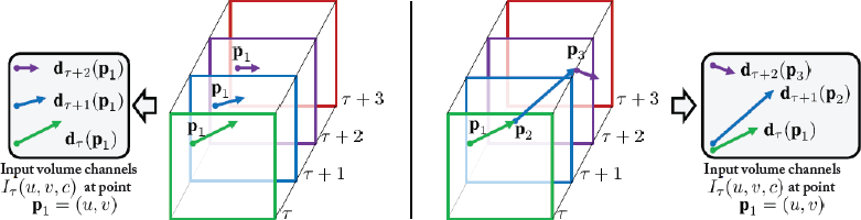
Architecture
The architecture of the two-stream CNNs model is shown in Fig. 7.21. The architecture of the spatial and temporal CNN models is similar, except that the second normalization layer is removed from the temporal CNN to reduce memory consumption. As shown in this figure, a class score fusion is added to the end of the model to combine the softmax scores of both the spatial and temporal models by late fusion. Different approaches can be used for class score fusion. However, experimental results showed that training a linear SVM classifier on stacked ℓ2-normalized softmax scores outperforms simple averaging.
7.6.3 LONG-TERM RECURRENT CONVOLUTIONAL NETWORK (LRCN)
Unlike the methods in Section 7.6.1 and Section 7.6.2 which learn CNN filters based on a stack of a fixed number of input frames, Long-term Recurrent Convolutional Network (LRCN) [Donahue et al., 2015] is not constrained to fixed length input frames and, thus, could learn to recognize more complex action video. As shown in Fig. 7.23, in LRCN, individual video frames are first passed through CNN models with shared parameters and then connected to a single-layer LSTM network (described in Chapter 3). More precisely, the LRCN model combines a deep hierarchical visual feature extractor, which is a CNN feature extractor, with an LSTM that can learn to recognize the temporal variations in an end-to-end fashion.
In this chapter, we discussed representative works, which use CNNs in computer vision. In Table 7.1, we provide an overview of some of the other important CNN applications and the most representative recent works, which have not been covered in detail in this book. In the following chapter, we will discuss some prominent tools and libraries of CNN.
Table 7.1: Few recent/most representative applications of CNN, not discussed in this book
Applications |
Paper Title |
Image captioning |
• Deep Visual-Semantic Alignments for Generating Image Descriptions [Karpathy and Fei-Fei, 2015] • DenseCap: Fully Convolutional Localization Networks for Dense Captioning [Johnson et al., 2016] |
3D reconstruction from a 2D image |
• Large Pose 3D Face Reconstruction from a Single Image via Direct Volumetric CNN Regression [Jackson et al., 2017] • Semantic Scene Completion from a Single Depth Image [Song et al. 2017] |
Contour/edge detection |
• DeepContour: A Deep Convolutional Feature Learned by Positive Sharing Loss for Contour Detection [Shen et al., 2015b] • Edge Detection Using Convolutional Neural Network [Wang, 2016] |
Text detection and recognition |
• Reading Text in the Wild with Convolutional Neural Networks [Jaderberg et al., 2016] • End-to-End Text Recognition with Convolutional Neural Networks [Wang et al., 2012] |
Octree representation for shape analysis |
• O-CNN: Octree-based Convolutional Neural Networks for 3D Shape Analysis [Wang et al., 2017] • OctNet: Learning Deep 3D Representations at High Resolutions [Riegler et al., 2016] |
Face recognition |
• DeepFace: Closing the Gap to Human-Level Performance in Face Verification [Taigman et al., 2014] • FaceNet: A Unified Embedding for Face Recognition and Clustering [Schroff et al., 2015] |
Depth estimation |
• Learning Depth from Single Monocular Images Using Deep Convolutional Neural Fields [Liu et al., 2016] • Deep Convolutional Neural Fields for Depth Estimation from a Single Image [Liu et al., 2015] |
Pose estimation |
• PoseNet: A Convolutional Network for Real-Time 6-DOF Camera Relocalization [Kendall et al., 2015] • DeepPose: Human Pose Estimation via Deep Neural Networks [Toshev and Szegedy, 2014] |
• Hedged Deep Tracking [Qi et al., 2016b] • Hierarchical Convolutional Features for Visual Tracking [Ma et al., 2015] |
|
Shadow detection |
• Automatic Shadow Detection and Removal from a Single Image [Khan et al., 2016a] • Shadow Optimization from Structured Deep Edge Detection [Shen et al., 2015a] |
Video summarization |
• Highlight Detection with Pairwise Deep Ranking for First-Person Video Summarization [Yao et al., 2016] • Large-Scale Video Summarization Using Web-Image Priors [Khosla et al., 2013] |
Visual question answering |
• Multi-level Attention Networks for Visual Question Answering [Yu et al., 2017] • Image Captioning and Visual Question Answering Based on Attributes and External Knowledge [Wu et al., 2017] |
Event detection |
• DevNet: A Deep Event Network for multimedia event detection and evidence recounting [Gan et al., 2015] • A Discriminative CNN Video Representation for Event Detection [Xu et al., 2015] |
Image retrieval |
• Collaborative Index Embedding for Image Retrieval [Zhou et al., 2017] • Deep Semantic Ranking Based Hashing for Multi-Label Image Retrieval [Zhao et al., 2015a] |
Person re-identification |
• Recurrent Convolutional Network for Video-Based Person Reidentification [McLaughlin et al., 2016] • An Improved Deep Learning Architecture for Person Re-Identification [Ahmed et al., 2015] |
Change detection |
• Forest Change Detection in Incomplete Satellite Images with Deep Neural Networks [Khan et al., 2017c] • Detecting Change for Multi-View, Long-Term Surface Inspection [Stent et al., 2015] |

1Since the total stride for both ZF and VGG nets on the last convolutional layer is 16 pixels.
2Equal to the number of classes in the PASCAL VOC dataset plus the background class.
3The 32 pixel stride is used to output a dense prediction at the same scale as the input image.
4The original FCN shown in Fig. 7.6 initialized with AlexNet model and the extended FCN shown in Fig. 7.7 initialized with VGGnet-16 model.
5Training these networks requires relatively more training data, time, and memory.
6Label prediction for large objects are obtained from only local information. Thus, the pixels which belong to the same large object may have inconsistent labels. Moreover, the pixels which belong to small objects may be classified as background.
7A convolutionalized VGGnet-16 is obtained by converting all the fully-connected layers to convolution layers.
8The stride of pool4 and pool5 layers in the original VGGnet-16 is 2.
9Instead of using transposed convolutional layers as in FCN and DDN, DeepLab uses a fast bilinear interpolation layer without training its parameters. This is because, unlike FCN and DDN, the output class score prediction maps of DeepLab (i.e., the output maps of conv8 layer) are quite smooth and thus a single up-sampling step can efficiently recover the output prediction maps with the same size as the input image
10In the minimax game, there are two players (e.g., generator and discriminator) and in all states the reward of player 1 is the negative of reward of player 2. Specifically, the discriminator minimizes a cross-entropy, but the generator maximizes the same cross-entropy.
11At the start of the training, the generator likely produces random samples, which are quite different from the real samples, so the discriminator can easily classify the real and fake samples.