19.1. Introduction

Divide and Conquer is a popular algorithm design strategy that has been widely used over a variety of problem classes. As the name indicates, the strategy solves a problem by dividing it repeatedly into smaller sub-problems, until the smaller sub-problems can be individually and easily solved. The strategy then backtracks, combining the solutions of the smaller sub-problems phase by phase on its return, until the solution to the original problem is automatically constructed, thereby conquering the problem. Needless to say, Divide and Conquer has been a time-tested political strategy too!

The fact that the strategy repeatedly moves onward to “divide” the problem and backtracks to “conquer” its solution, is suggestive of the application of recursion. Thus, Divide and Conquer-based solutions to problems are ideally implemented as recursive procedures or programs (see section 2.7 of Chapter 2, Volume 1, for a discussion on recursion and analysis of recursive procedures).

19.2. Principle and abstraction

Figure 19.1(a) illustrates the principle of Divide and Conquer, where a problem whose data set size is n, is repeatedly divided into smaller sub-problems each of which are solved independently, before the principle backtracks to combine the solutions of the sub-problems, to finally arrive at the solution to the original problem.

Figure 19.1(b) illustrates the abstraction of the Divide and Conquer method. The function SMALL(r,t) determines if the size of the sub-problem whose data set size is given by (r,t), is small enough to be solved independently and directly using the function B(r,t). Note that the if condition functions as the base case of the recursive procedure. DIVIDE(r,t) divides the problem into two sub-problems of smaller sizes and the function COMBINE() combines the solutions of the two sub-problems. The repeated division of the problem is handled recursively, by calling DIVIDEandCONQUER() over the sub-problems.

The application of the Divide and Conquer method for the solution of problems is detailed in the ensuing sections.

19.3. Finding maximum and minimum

Finding the maximum and minimum elements in a list, termed the max-min problem for ease of reference, is a simple problem. While there are different methods available to solve this problem, we use this problem only to demonstrate how Divide and Conquer works to obtain its solution.

Procedure MAXMIN()(Algorithm 19.1) illustrates the pseudo-code for the Divide and Conquer-based solution to the max-min problem. The procedure begins with the original dataset D and recursively divides the dataset D into two subsets D1 and D2, that comprise half the elements of D. To undertake this, the recursive procedure is called twice, one as MAXMIN(D1) and the other as MAXMIN(D2).

The base cases of the recursive procedure are invoked when the divided dataset comprises just two elements {a, b} at which point, the max and min elements are computed by a mere comparison of the elements, or when the divided dataset comprises a single element {a} at which point, both the max and min elements are set to {a} and returned to their respective calling procedures. When recursion terminates, (MAX1, MIN1) and (MAX2, MIN2) store the max and min elements of D1 and D2, respectively.

One last comparison between the max elements and the min elements returns the final maximum and minimum element of the given dataset, at which point recursion terminates successfully.

Illustrative problem 19.1 demonstrates the working of procedure MAXMIN() over a problem instance.

19.3.1. Time complexity analysis

Since procedure MAXMIN() is a recursive procedure, to obtain the time complexity of the procedure, the recurrence relation needs to be framed first. Since there are two recursive calls in the procedure, for an input size n, the time complexity T(n) expressed in terms of the element comparisons made over the data set is given by the following recurrence relation:

[19.1]

The base case (n = 1), does not entail any element comparisons, hence T(n) = 0, whereas, the base case (n = 2) entails only one comparison between a and b to determine the max and min elements and therefore T(n) = 1. For (n > 2), the two recursive calls incur a time complexity of with two more comparisons undertaken last, to determine the final maximum and minimum element of the data set.

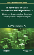
Solving equation [19.1] assuming that n = 2^k for some k, yields,

In the i^th step,

Since n = 2^k, in the step when i = (k-1),

Thus, the time complexity of the Divide and Conquer-based max/min element finding problem is O(n).

19.4. Merge sort

The merge sort algorithm which makes use of the principle of merge to order a data set was discussed in section 17.5. Algorithm 17.5 illustrates the recursive merge sort algorithm (procedure MERGE_SORT). The merge sort algorithm employs a Divide and Conquer approach to sort the elements.

Thus, the original list is divided into two sub-lists and the recursive MERGE_SORT procedure is invoked over the two sub-lists after which the two sorted sub-lists are merged one last time using procedure MERGE (Algorithm 17.4 in section 17.5), yielding the sorted list.

19.4.1. Time complexity analysis

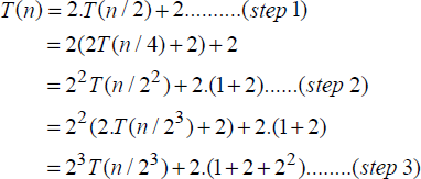
The recurrence relation for the time complexity of procedure MERGE_SORT is given by,

where c and d are constants. Illustrative problem 17.5, shows the solution of the recurrence relation, yielding a time complexity of O(n.log₂ n).

19.5. Matrix multiplication

The multiplication of two square matrices A, B of order n, is given by,

where

Known as the “high school” method, this way of multiplying two square matrices involves three for loops, two to keep the indices i, j of C_ij running and the third running over index k, to sum up the product (a_ik. b_kj). With all the three loops ranging from 1 to n, where n is the size of the square matrices, the time complexity of the iterative algorithm is bound to be O(n³).

Now, what if a Divide and Conquer-based approach was adopted to undertake this “high school” method of computing the product of two square matrices? Would it result in a better time complexity? Let us explore.

19.5.1. Divide and Conquer-based approach to “high school” method of matrix multiplication

A Divide and Conquer-based approach could involve dividing the square matrices A and B into four quadrants A₁₁, A₁₂, A₂₁, A₂₂ and B₁₁, B₁₂, B₂₁, B₂₂ respectively, as shown in Figure 19.2 and recursively undertaking the division of each of the quadrants into four other “miniature” quadrants and so on, until each of the quadrants is just left with a 2 ×2 matrix. At this stage, the base case of the recursive procedure merely does the usual “high school” method of matrix multiplication and returns the results, which eventually results in the recursive procedure returning the product of the two matrices as (C)n X n.

The governing recurrence relations of the Divide and Conquer-based algorithm are as follows:

[19.2]

where A_ij, B_ij and C_ij denote sub-matrices of order and a_ij, b_ij and c_ij denote matrix elements. A_ij.B_jk in general denotes the recursive matrix multiplication of the sub-matrices of until the base case is triggered at n = 2, at which stage the matrix multiplication of two matrices of order 2 × 2 is undertaken as illustrated in equation [19.2].

19.5.1.1. Time complexity analysis

The time complexity of the Divide and Conquer-based “high school” method of matrix multiplication in terms of the basic operations, i.e. the matrix additions and multiplications that were carried out during recursion, are obtained as follows.

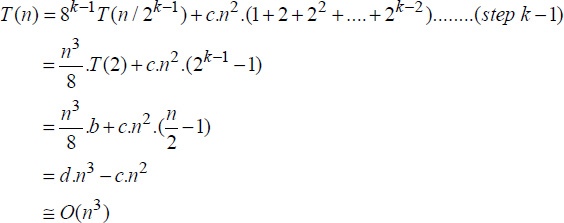
Let T(n) denote the time complexity of multiplying two square matrices of order n. The recursive algorithm calls for eight matrix multiplications and four matrix additions of sub-matrices of order , during each call. When n = 2, it reduces to eight element multiplications and four element additions. The recurrence relation is therefore given by,

[19.3]

Since the addition of two square matrices of order n has a time complexity of O(n²), c.n² in equation [19.3] denotes the upper bound for the four matrix additions called for, by the recursive algorithm.

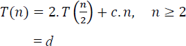
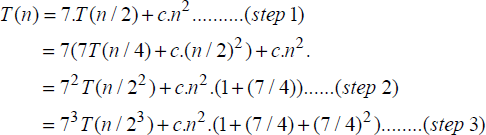
Solving equation [19.3] assuming that n = 2^k for some k, yields,

In the ith step,

Since n = 2^k, in the step when i = (k-1),

Thus, despite the Divide and Conquer-based approach, the “high school” method of matrix multiplication does not yield a performance better than its traditional method of element multiplications and additions, which also yielded O(n³) time complexity.

19.5.2. Strassen’s matrix multiplication algorithm

Strassen’s matrix multiplication algorithm devised by Volker Strassen is a faster matrix multiplication method when compared to the traditional method. It works best over large matrices, though not as much as other competing methods.

Adopting a Divide and Conquer-based approach, the algorithm recursively divides the matrices A and B into four quadrants as shown in Figure 19.2, and proceeds to compute the intermediary matrices P, Q, R, S, T, U and V, to obtain the final matrix C.

[19.4]

Strassen’s method recursively works on equation [19.4] until the base case of n = 2 is reached. At this stage, as discussed with regard to equation [19.2], the computations become element additions, subtractions and multiplications.

An observation of equation [19.4] reveals that the algorithm uses seven matrix multiplications and 18 matrix additions/subtractions. Thus, the method seems to have saved on one matrix multiplication when compared to the traditional method but in the process has jacked up the matrix additions/subtractions to a whopping eighteen! Will it ensure good performance? Let’s explore its time complexity.

19.5.2.1. Time complexity analysis

Following a similar description of T(n) in equation [19.3], the recurrence relation for Strassen’s method is as follows:

[19.5]

c.n² in the equation denotes the upper bound for the eighteen matrix additions/subtractions called for, by the recursive algorithm.

Solving equation [19.5] using the usual steps and assuming that n = 2^k for some k, yields,

In the i^th step,

Since n = 2^k, in the step when i = (k-1),

Thus, the Divide and Conquer-based on Strassen’s method for matrix multiplication reports a time complexity of O(n^2.81), which is a better performance especially for large matrices, when compared to the time complexity of O(n³) reported by the “high school” method.

19.6. Illustrative problems