
21
Dynamic Programming
In this chapter, the algorithm design technique of Dynamic Programming is detailed. The technique is demonstrated over 0/1 Knapsack Problem, Traveling Salesperson Problem, All-Pairs Shortest Path Problem and Optimal Binary Search Tree Construction.
21.1. Introduction
Dynamic Programming is an effective algorithm design technique built on Bellman’s Principle of Optimality which states that ‘an optimal sequence of decisions has the property that whatever the initial state and decisions are, the remaining decisions must constitute an optimal decision sequence with regard to the state resulting from the first decision’.
The dynamic programming strategy is applicable to optimization problems, which comprise an objective function that needs to be maximized or minimized, subject to constraints that need to be satisfied. A candidate solution that satisfies the constraints is termed a feasible solution and when a feasible solution results in the best objective function value, it is termed an optimal solution.
The greedy method (discussed in Chapter 20) also works over problems whose characteristics are as defined above and obtains optimal solutions to these problems. How then is a greedy method different from dynamic programming?
A greedy method works in an iterative fashion, selecting objects constituting the solution set one by one and constructing a feasible solution set, which eventually turns into an optimal solution set. However, there are problems where generating a single optimal decision sequence is not always possible and therefore, a greedy method might not work on these problems.
It is here that dynamic programming finds its rightful place. Dynamic programming, unlike the greedy method, generates multiple decision sequences using Bellman’s principle of optimality and eventually delivers the best decision sequence that leads to the optimal solution to the problem. Also, dynamic programming ensures that any decision sequence that is being enumerated but does not show promise of being an optimal solution is not generated. Thus, to favor the enumeration of multiple decision sequences, dynamic programming algorithms are always recursive in principle.
Let P(1, n) denote a problem, which demands an optimal sequence of n decisions as its solution, with an initial problem state S0. Let (x1, x2,...xn) be the n decision variables with regard to the problem. Let us suppose that from among a set of k decisions {d1, d2,...dk} available for decision variable x1, a decision x1 = dj was taken, which results in a problem state S1. According to the principle of optimality, whatever be the decision dj taken on x1, the remaining decision sequence pertaining to decision variables (x2, x3, ...xn) must constitute an optimal sequence with regard to the problem state S1.
Generalizing, if Si is the respective problem state following each of the decisions di, 1 ≤ i ≤ k, for the decision variable x1, and Γi are the optimal decision sequences with regard to the rest of the decision variables, for the problem states Si, then according to the principle of optimality the final optimal decision sequence with regard to the problem whose initial state is S0, is the best of the decision sequences, diΓi, 1 ≤ i ≤ k.
It is therefore quite obvious that dynamic programming generates many decision sequences, but the strategy employing the principle of optimality ensures that those sequences which are sub-optimal are not generated, as far as possible. In the worst case, if there are n decision variables each of which has d choices for their respective decisions, then the total number of decision sequences generated would be dn, which is exponential in nature. Despite this observation, dynamic programming algorithms for most problems have reported polynomial time complexity considering the fact that the sub-optimal decision sequences are not generated by the strategy.
It is prudent to apply the principle of optimality in a recursive fashion considering the large sequence of decisions that are generated, each with regard to the problem states arising out of the earlier decisions that are taken. Hence, dynamic programming algorithms are always governed by recurrence relations, solving which one can easily attain the optimal decision sequence for the problem concerned. Adhering to the norms of recursion, the base cases for the recurrence relations need to be constructed from the respective problem definitions.
The solution of the recurrence relations defining a dynamic programming algorithm can be undertaken in two ways, viz., forward approach and backward approach.
In the forward approach, if (x1, x2, ...xn) are the n decision variables on which an optimal decision sequence has to be constructed, then the decision on xi is made in terms of the optimal decision sequences for xi+1, xi+2, ...xn. On the contrary, in the backward approach, the decision on xi is made in terms of the optimal decision sequences for x1, x2, ...xi-1. Thus, the forward approach deals with “look ahead” decision making and the backward approach deals with “look back” decision making.
In practice, formulating the recurrence relation for a problem works out easier, when a backward approach is followed. The recurrence relation, however, is solved forwards. For a forward approach based on recurrence relation, the solution of the relation becomes easier when backward solving is undertaken beginning with the last decision.
Another important characteristic of dynamic programming strategy is that the solutions to sub-problems obtained by the respective optimal decision subsequence are preserved thereby avoiding re-computation of values. Therefore, in most cases, the values computed by the recurrence relations can be tabulated, which permits the effective transformation of a recursive process into iterative program code, while implementing dynamic programming algorithms. Thus, most dynamic programming algorithms can be expressed as iterative programs.
The ensuing sections demonstrate the application of dynamic programming to the problems of 0/1 knapsack, traveling salesperson, all-pairs shortest paths and optimal binary search trees.
21.2. 0/1 knapsack problem
The 0/1 knapsack problem is similar to the knapsack problem discussed in section 20.2 of Chapter 20, but with the difference that none of the objects selected may be dismantled while pushing them into the knapsack. In other words, xi the proportion of objects selected could be either 1 when the object is fully selected for inclusion in the knapsack, or 0, when the object is rejected for it does not completely fit into the knapsack.
The 0/1 knapsack problem is therefore defined as:

subject to
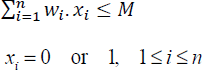
where, O1, O2, … On indicate n objects, and (p1, p2, … pn) and (w1, w2, … wn) represent their profits and weights, respectively. Here, M is the capacity of the knapsack and (x1, x2, … xn) are the proportion of objects selected, which can be either 0 or 1. The objective is to determine the sequence of objects which will fit into the knapsack and yield maximum profits.
How does dynamic programming work to obtain the recurrence relation that will help obtain the optimal decision sequence?
21.2.1. Dynamic programming-based solution
Let KNAP0/1 (1, n, M) indicate the 0/1 knapsack problem instance, which demands n optimal decisions with regard to its selection of objects that fit into a knapsack whose capacity is M. With regard to x1, there can only be two decisions. If (x1 = 0) then the first object is rejected and therefore the optimal decision sequence involves solving the sub-problem KNAP0/1(2, n, M). If (x1 = 1) then the first object is selected and therefore the optimal decision sequence involves solving the sub-problem KNAP0/1(2, n, M-w1).
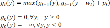
Let gj(y) be the optimal solution (maximal profits) to the sub-problem KNAP0/1(j+1, n, y). The objective is to obtain the optimal solution g0(M) to the original problem KNAP0/1 (1, n, M). There can only be two decisions with regard to the first decision on x1, viz., x1 = 0 or x1 = 1. Following the principle of optimality, g0(M) can be computed as:
Here g1(M) denotes the optimal solution to the rest of the sub-problem, with no profits accrued so far and with M intact, on account of the first decision x1 = 0. g1(M-w1) + p1 denotes the optimal solution to the rest of the sub-problem with a profit of p1 gained already and a decreased capacity of M-w1, on account of the first decision x1 = 1. Generalizing to accommodate the optimal solutions with regard to intermediary sequences for the sub-problems concerned:
It can be seen that the recurrence relation [21.3] models a forward approach and the base cases can be framed using the knowledge that gn(y) = 0, ∀ y, since n decisions have already been taken by then and therefore there are no profits to be earned.
Solving backward beginning with gn(y), we obtain gn-1(y) by substituting i = n-1 in equation [21.3], from gn-1(y) we obtain gn-2(y) and so on until we finally arrive at g0(M) that yields the optimal solution to the 0/1 knapsack problem.
A backward approach to the dynamic programming algorithm for the 0/1 knapsack problem, would try to compute gn(M) as the optimal solution to the problem KNAP0/1(1, n, M), yielding the following recurrence relation:
Tracking which among the two decisions gave the maximum value can help fix the value of the decision variable xi concerned. Thus, g3(60) obtains its maximum value from g2(20) + 50, which decides on including the object w3 = 40 into the knapsack and therefore sets x3 = 1. Proceeding in a similar way, the optimal values of the decision variables turn out to be (x1, x2, x3) = (1, 0, 1). The maximum profit earned is 60 with the knapsack capacity utilized to be 60.
21.3. Traveling salesperson problem
The traveling salesperson problem deals with finding the optimal cost of undertaking a tour that begins with a city, visiting all other cities charted out in the tour once, without revisiting any one of them again, before returning to the city from where the tour started.
Let G = (V, E) where V is the set of vertices and E is the set of edges, be a weighted digraph with cij indicating the cost (weight) of edge <i, j>. Let |V| = n, n >1 be the number of vertices. The cost matrix (cij) n X n is defined as cij > 0, for all i and j, and cij = ∞, if edge <i, j> does not exist in E.
A tour of G is a directed cycle that begins from a vertex S and includes all other vertices of G before it ends in vertex S. The cost of the tour is the sum of the costs of all the edges. A minimum cost tour is a tour that reports the minimal cost. The traveling salesperson problem concerns finding the minimum cost tour from a source node S.
21.3.1. Dynamic programming-based solution
The recurrence relation of the dynamic programming-based solution for the traveling salesperson problem can be framed as follows.
Let g(x, y) denote the minimum cost of the tour undertaken from node x, traveling through all other nodes in y before ending the tour at the source node S. Without loss of generality, let us suppose that V = {1, 2, 3, …n} are the n nodes in the weighted digraph and node {1} is the source node.
Following the principle of optimality, the recurrence relation to obtaining the minimum cost tour is given by:
To obtain g(1, V-{1}), a series of decision sequences with regard to the tour moving over to the next node k, 2 ≤ k ≤ n from the source node, need to be recursively computed.
Generalizing, for i ∉ T:
Equation [21.6] can now be used to undertake recursive computations for the intermediary decision sequences. The base case is reached when there are no more nodes to visit during the tour before ending the tour at the source node {1}. The base cases are therefore given by:
21.3.2. Time complexity analysis and applications of traveling salesperson problem
The number of g(i, T) functions that are computed before equation [21.5] is used to compute g(1, V-{1}) is given by:

This is so since for each set T during the intermediary computations, there are (n-1) choices for i. Therefore, the number of distinct sets of T, excluding 1 and i is ![]() . Each g(i, T) requires (k-1) comparisons when the cardinality of the set T is k. Hence, the time complexity is given by Θ(n2. 2n).
. Each g(i, T) requires (k-1) comparisons when the cardinality of the set T is k. Hence, the time complexity is given by Θ(n2. 2n).
The traveling salesperson problem finds its application in areas such as planning, scheduling, vehicle routing, logistics and packing, robotics and so forth.
21.4. All-pairs shortest path problem
The all-pairs shortest path problem deals with finding the shortest path between any pair of cities given a network of cities.
Let G = (V, E) be a weighted digraph with n vertices represented by V and edges <i, j> represented by E. Let (C)n×n denote the cost (weight) matrix where Cij = 0, for i = j and Cij = ∞, for < i.j > ∉ E. The all-pairs shortest path problem concerns such a graph G = (V, E) where the vertices V represent cities and the edges E represent the connectivity between the cities, and the cost matrix (C)n×n represents the distance matrix between the cities. Thus, Cij denotes the distance between the cities represented by vertices i and j.
It is possible that the distance between two cities i, j connected by a direct edge, can be longer than a path i→k→j, where k is an intermediate city between i and j. The solution to the all-pairs shortest path problem is to obtain a matrix S which gives the minimum distance between cities i and j.
It is possible to solve the all-pairs shortest path problem by repeatedly invoking Dijkstra’s single source shortest path algorithm (discussed in section 9.5.1 of Chapter 9, Volume 2) n times, with each city i as the source, thereby obtaining the shortest paths from city i to all other cities. However, Floyd’s algorithm which will be introduced in the ensuing section employs the principle of optimality over the cost matrix (C)n×n and obtains the optimal matrix S which obtains the minimum distance between any two cities, in one run.
21.4.1. Dynamic programming-based solution
Floyd’s algorithm adopts dynamic programming to solve the all-pairs shortest path problem. Let Sk(i,j) represent the length of the shortest path from node i to node j passing through no vertex of index greater than k. Then the paths from i to k and k to j must also be shortest paths not passing through a vertex of index greater than (k-1). Making use of this observation, the recurrence relation is framed as:

Algorithm 21.1 Floyd’s algorithm for the all-pairs shortest path problem
The shortest path from i to j that does not go through a vertex higher than k, either goes through a vertex k or it does not. If it goes through k, then Sk(i, k) = Sk−1(k, j) and if it does not go through k, then Sk(i, j) = Sk−1(i, j), which explains the recurrence relation for k ≥1.
On the other hand, when k = 0, the shortest path is given by the edges connecting i and j, for all i and j, that is Cij, which are the base cases for the recurrence relation.
Algorithm 21.1 illustrates Floyd’s algorithm, which employs the recurrence relation described in equation [21.8] to obtain the optimal distance matrix S, which is the solution to the all-pairs shortest path problem.
21.4.2. Time complexity analysis
Floyd’s algorithm illustrated in Algorithm 21.1, is an iterative implementation of its governing recurrence relations described by equation [21.8]. It is therefore easy to see that the three for loops each running from 1 to n, yield a time complexity of Θ(n3). However, while Algorithm 21.1 is a naïve rendering of the recurrence relations as they are, it is possible to achieve a speed up by cutting down on the computations and comparisons, in the innermost loop.
21.5. Optimal binary search trees
Binary search trees were detailed in Chapter 10, Volume 2. To recall, a binary search tree is a binary tree that can be empty or if non-empty, comprises distinct identifiers representing nodes that satisfy the property of the left child node identifier being less than its parent node identifier and the right child node identifier being greater than its parent node identifier. This leads to the characteristic that all the identifiers in the left subtree of the binary search tree are less than the identifier in the root node and all the identifiers in the right subtree of the binary search tree are greater than the identifier in the root node.
Figure 21.3 illustrates an example binary search tree representing the keys {h, r, e, k, a, f, c, z}. It can be observed that with h as the root node, the keys {a, c, e, f} which form the left subtree are less than key h of the root node and the keys {k, r, z} which form the right subtree are greater than the key h of the root node. Besides, each parent node key is such that the left child node key is less than itself and the right child node key is greater than itself.
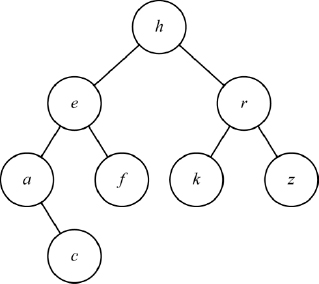
Figure 21.3 An example binary search tree
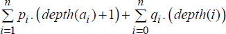
Given a set of keys, for each permutation or arrangement of the keys in the list, a binary search tree can be constructed resulting in a variety of binary search tree structures each with its own behavioral characteristics. Thus, each binary search tree could be associated with a cost with regard to successful/unsuccessful searches performed on them, as discussed in illustrative problem 10.4, in Chapter 10, Volume 2. To recollect, if S = {a1, a2, a3, … an} is a set of keys and Tk are the set of associated binary search trees that can be constructed out of S, then the cost of a binary search tree is given by:
where pi, 1 ≤ i ≤ n, is the probability with which ai is searched for (probability of successful search) and qj, 0 ≤ j ≤ n, is the probability with which a key X, aj ≤ X ≤ aj+1 is unsuccessfully searched for (probability of unsuccessful search) on a binary search tree Tk.
The cost of the binary search tree can also be defined in terms of the depth of the nodes as:
where depth(i) indicates the depth of the external nodes indicated as squares, at which the unsuccessful search logically ends (see section 10.2, Chapter 10, Volume 2, for more details).

Dynamic programming helps to obtain the optimal binary search tree by working over decision sequences and applying the principle of optimality, to select the right node at each stage which will ensure minimal cost.
21.5.1. Dynamic programming-based solution
Given the list of keys S = {a1, a2, a3, … an} and the probabilities pi, 1 ≤ i ≤ n, and qj, 0 ≤ j ≤ n the objective is to obtain the optimal binary search tree using dynamic programming.
Let Tij be the minimum cost tree for the subset of keys Sij = {ai+1, ai+2, ai+3 … aj} with cost Cij and root Rij. By this description and notation, Tii denotes an empty tree with cost Cii = 0. Let the weight Wij of Tij be defined as:
The weight Wii of the empty tree Tii would be qi.
The tree Tij consists of a root ak, i ≤ k ≤ j with its left subtree Tik-1 representing the minimum cost tree for keys Sik−1 = {ai+1, ai+2, ai+3, … ak−1} and right subtree Tkj representing the minimum cost tree for keys Skj = {ak+1, ak+2, ak+3, … aj}, as shown in Figure 21.4.
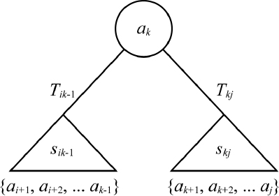
Figure 21.4 Composition of minimum cost tree Tij
It can be inferred that when (i = k-1) the left subtree is empty and when (k = j) the right subtree is empty.
The construction of Tij with ak, Tik-1 and Tkj, results in the depth of nodes in the left and right subtrees of Tij increasing by 1, in respect of their earlier depths when they belonged to Tik-1 and Tkj. The cost Cij of Tij defined by equation [21.10], can now be written as:
Since:
we obtain:
To find the optimal cost tree Tij, we need to choose the root node ak, i < k ≤ j with Tik-1 and Tkj as the left and right subtrees, compute the cost and then select the tree with the minimal cost. Therefore, the recurrence relation that computes the minimal cost tree is given by:
The minimum cost tree T0n for the list S = {a1, a2, … an} can be obtained by solving for C0n from the equation [21.15]. The base cases for the recurrence relation are given by Cii = 0 and Wii = qi, 0 ≤ i ≤ n. To compute Wij in equation [21.15] easily, the following equation derived from equation [21.11] by mere manipulation of the terms, can be used effectively.
21.5.2. Construction of the optimal binary search tree
The optimal binary search tree T0n for n keys can be easily constructed by tracking that index k at which point mini<k≤j(Cij−1 + Ckj) attains its minimum value in equation [21.15], while computing the cost Cij for the subtree Tij. Thus, the root Rij for the subtree Tij is ak. This means that the left subtree Tik-1 of ak shall comprise the keys {ai+1, ai+2, … ak-1} and the right subtree Tk, j shall comprise the keys {ak+1, ak+2, … akn}, whose root nodes concerned will be arrived at, following similar arguments and computations. Eventually, when C0n is computed, R0n = ak denotes the root node of the optimal binary search tree represented by T0n.
Algorithm 21.2 illustrates the procedure to obtain the optimal binary search tree, given the list of keys S = {a1, a2, a3, … an} and the probabilities pi, 1 ≤ i ≤ n and qj, 0 ≤ j ≤ n.

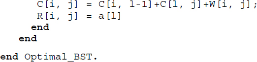
Algorithm 21.2 Dynamic programming-based solution to optimal binary tree construction
The demonstration of procedure Optimal_BST on a list of keys with known probabilities of successful search and unsuccessful search has been illustrated in example 21.5. It can be seen that the computations with regard to the recurrence relation described by equation [21.15] have been organized in the increasing order of value of j –i, as specified in the algorithm.
21.5.3. Time complexity analysis
The time complexity of the optimal binary search tree construction can be easily arrived at by observing the loops in the procedure Optimal_BST. The major portion of the time is consumed at the point where the recurrence relation of the dynamic programming-based solution is executed. This concerns finding that k which minimizes Cik-1 + Ckj, 1<k ≤ j. The loop executing this requires O(j-i) time. The outer loop in the second for statement works n times and the inner loop works at most n times for each iteration of the outer loop. Hence, the time complexity of the construction of an optimal binary search tree is O(n3).
Summary
- Dynamic programming works over Bellman’s Principle of Optimality.
- The method works over optimization problems defined by an objective function and constraints. It obtains the optimal solution to the problem.
- Dynamic programming unlike the greedy method, generates many decision sequences before the optimal decision sequence is delivered as the solution. The greedy method, in contrast, generates only one decision sequence.
- Dynamic programming is governed by recurrence relations which can be solved by adopting a backward approach or a forward approach.
- The method has been demonstrated over the problems of 0/1 knapsack, traveling salesperson, all-pairs shortest path and optimal binary search tree construction.
21.6. Illustrative problems
Review questions
- Define the principle of optimality.
- Distinguish between dynamic programming and greedy method ways of problem-solving.
- The backward approach to solving the 0/1 knapsack problem has been defined by equation [21.4] in this chapter. Trace the approach over the 0/1 knapsack instance discussed in example 21.1 of this chapter.
- Obtain the recurrence relation of the dynamic programming-based solution to the traveling salesperson problem.
- Solve the following traveling salesperson problem assuming that the cost matrix of the vertices V = {1, 2, 3, 4, 5} is as given below:

- Outline the dynamic programming-based algorithm for the all-pairs shortest path problem.
- Obtain the solution to the all-pairs shortest path problem with four cities {a, b, c, d} whose distance matrix is as given below:

- Construct an optimal binary search tree for the keys {l, u, w, m} with probabilities of successful and unsuccessful search given by (p1, p2, p3, p4) = (4/20, 3/20, 5/20, 1/20) and (q0, q1, q2, q3, q4) = (1/20, 2/20, 1/20, 2/20, 1/20), respectively.
Programming assignments
- Implement Algorithm 21.1
procedureFLOYDand test it over the problem instance shown in review question 7. - Implement Algorithm 21.2
procedureOptimal BSTand test it over the problem instance shown in review question 8.