Search in book...
Toggle Font Controls
Create new playlist

Name your new playlist

Playlist description (optional)
Sign In

Email address

Password

Forgot Password?

or

Continue with Facebook

Continue with Google
Sign Up

Full Name

Email address

Confirm Email Address

Password

or

Continue with Facebook

Continue with Google

20
Greedy Method

This chapter discusses the greedy method and demonstrates the strategy over the Knapsack problem, Prim’s and Kruskal’s spanning tree extraction algorithms and Dijkstra’s Single Source Shortest Path problem.

20.1. Introduction

The greedy method is an algorithm design technique, which is applicable to problems defined by an objectivefunction that needs to be maximized or minimized, subject to some constraints. Given n inputs to the problem, the aim is to obtain a subset of n, that satisfies all the constraints, in which case it is referred to as a feasible solution. A feasible solution that serves to obtain the best objective function value (maximal or minimal) is referred to as the optimal solution.

The greedy method proceeds to obtain the feasible and optimal solution, by considering the inputs one at a time. Hence, an implementation of the greedy method-based algorithm is always iterative in nature. Contrast this with the implementation of Divide and Conquer based algorithms discussed in Chapter 19, which is always recursive in nature.

20.2. Abstraction

The abstraction of the greedy method is shown in Figure 20.1. Here, the function SELECT(A) makes a prudent selection of the input depending on the problem. Function FEASIBLE() ensures that the solution satisfies all constraints imposed on the problem and AUGMENT() augments the current input which is a feasible solution to the solution set. Observe how the for loop ensures consideration of inputs one by one, justifying the iterative nature of greedy algorithms.

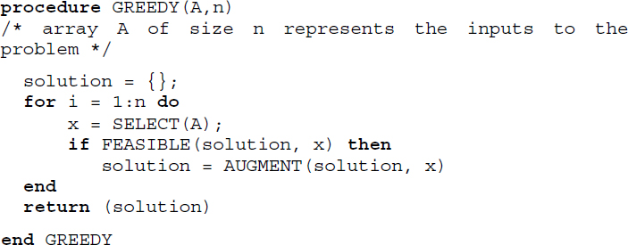
**Figure 20.1** *Abstraction of the greedy method*

The application of the greedy method in the design of solutions to the knapsack problem, extraction of minimum cost spanning trees using Prim’s and Kruskal’s algorithms and Dijkstra’s single source shortest path problem, are discussed in the ensuing sections.

20.3. Knapsack problem

The knapsack problem is a classic problem to illustrate the greedy method. The problem deals with n objects with weights (W₁, W₂, …W_n ) and with profits or prices (P₁, P₂, …P_n). A knapsack with a capacity of M units is available. In other words, the knapsack can handle only a maximum weight of M, when objects with varying weights are packed into it. A person is allowed to own as many objects, on the conditions that (i) the total weight of all objects selected cannot exceed the capacity of the knapsack and (ii) objects can be dismantled and parts of them can be selected.

From a practical standpoint, a person while selecting the objects would try to choose those that would fetch high profits, hoping to maximize the profit arising out of owning the objects. Thus, maximizing profit is the objective function of the problem. The fact that objects selected can be dismantled and that their total weight cannot exceed the capacity of the knapsack are the constraints.

Let (O₁, O₂, … O_n) be n objects, and (p₁, p₂, … p_n) and (w₁, w₂, … w_n) be their profits and weights, respectively. Let M be the capacity of the knapsack and (x₁, x₂, … x_n) be the proportion of objects which are selected. The mathematical formulation of the knapsack problem is as follows:

subject to

[20.1]

The objective function describes the maximization of the total profits. The constraints describe the total weight of the objects selected to be bound by M and the proportion of objects selected to lie between [0,1], where x_i = 0 denotes rejection, x_i = 1 denotes the selection of the whole object and anything in between [0, 1] denotes the selection of a part of the object after dismantling it.

20.3.1. Greedy solution to the knapsack problem

20.3.1.1. Strategy 1

A greedy solution to the knapsack problem involves selecting the objects one by one such that the addition of each object into the knapsack increases the profit value, subject to the capacity of the knapsack. This could mean ordering the objects in the non-increasing order of their profits and selecting them one by one until capacity M is exhausted. Will this strategy yield the optimal solution?

20.3.1.2. Strategy 2

Another “more-the-merrier” strategy could insist on ordering the objects in the non-decreasing order of their weights and pack as many objects as possible into the knapsack, subject to the capacity M, hoping to maximize profit by a larger selection of objects. Will this strategy yield the optimal solution?

20.3.1.3. Strategy 3

A third strategy could be to order the objects according to the non-increasing order of profit per unit weight (profit/weight), that is , and select objects one by one until the capacity M of the knapsack is exhausted. Will this strategy yield the optimal solution?

It can be observed that all the three strategies are greedy method based since they revolve around selecting the object one by one while trying to satisfy the constraints and aiming to maximize the objective function. Let us explore these strategies over an example knapsack problem.

EXAMPLE 20.1.–

Consider three objects O₁, O₂, O₃ with (p₁, p₂, p₃) = (25, 36, 34) and (w₁, w₂, w₃) = (20, 28, 25) describing their profits and their weights, respectively. Let M = 30 be the capacity of the knapsack and (x₁, x₂, x₃) be the proportion of objects which are selected. The optimal solutions delivered by the three strategies described above are as given below:

Greedy method	(x₁, x₂, x₃)	M
*Strategy 1*	(0, 1, 2/25)	30	38.72
*Strategy 2*	(1, 0, 10/25)	30	38.6
*Strategy 3*	(0, 5/28, 1)	30	40.43

Of the three strategies, it can be seen that strategy 3 which selects objects based on the highest profit per unit weight value, obtains the optimal solution.

In strategy 3, the greedy method orders the objects according to the profit per unit weight value and selects the objects or their proportions such that the capacity M of the knapsack is not exceeded, thereby satisfying the constraints imposed and therefore turning out a feasible solution. The optimal solution arrived at after evaluating the objective function value for the selected x_i s is 40.43, which is the best. It can be proved that a greedy method that works by selecting the objects based on their profit per unit weight value, for a given instance of the knapsack problem, will always yield the optimal best solution. The proof for this can be seen in illustrative problem 20.1.

Algorithm 20.1 (Procedure GREEDYMETHOD_KNAPSACK()) illustrates the working of strategy 3.

Algorithm 20.1 Greedy method solution for the knapsack problem

20.4. Minimum cost spanning tree algorithms

Given a connected undirected graph G = (V, E), where V is the set of vertices and E is the set of edges, a subgraph T = (V, E′), where E′ ⊆ E is a spanning tree if T is a tree.

It is possible to extract many spanning trees from a graph G. When G is a connected, weighted and undirected graph, where each edge involves a cost, then a minimum cost spanning tree is a spanning tree that has the minimum cost. Section 9.5.2 of Chapter 9, Volume 2, details the concepts and construction of minimum spanning trees using two methods, which are, Prim’s algorithm (Algorithm 9.4) and Kruskal’s algorithm (Algorithm 9.5).

Both the algorithms adopt the greedy method of algorithm design, despite differences in their approach to obtaining the minimum cost spanning tree.

20.4.1. Prim’s algorithm as a greedy method

Prim’s algorithm selects the minimum cost edge one by one, to optimize the cost of the spanning tree and proceeds to construct the spanning tree after ensuring that the inclusion of the edge does not violate the constraints of (i) edge forming a cycle and (ii) edge staying connected, with the spanning tree under construction. Once all the vertices V have made their appearances in the constructed spanning tree, the algorithm abruptly terminates discarding any leftover edges, while declaring the minimum cost spanning tree as its output.

Thus, in the case of Prim’s algorithm, the objective function is the minimization of the cost of the spanning tree and the constraints ensure the connectedness and acyclicity of the spanning tree, when each edge is added to the tree. The algorithm adopts the greedy method of design by selecting the edges one by one while working to obtain the feasible solution at every stage until the optimal solution is arrived at in the final step.

The time complexity of Prim's algorithm is O(n²), where n is the number of vertices in the graph.

20.4.2. Kruskal’s algorithm as a greedy method

Kruskal’s algorithm, on the other hand, selects a minimum cost edge one by one, just as Prim’s algorithm does, but with a huge difference in that, the selected edges build a forest and not necessarily a tree, during the construction. However, the selection of edges ensures that no cycles are formed in the forest.

Kruskal’s algorithm, therefore, works over a forest of trees until no more edges can be considered for inclusion and the number of edges in the forest equals (n-1), at which stage, the algorithm terminates and outputs the minimum cost spanning tree that is generated.

Thus, in the case of Kruskal’s algorithm, the objective function is the minimization of the cost of the spanning tree and the constraint ensures the acyclicity of trees in the forest. The algorithm also adopts the greedy method of design where the edges are selected one by one, obtaining the feasible solution at each stage until the optimal solution, which is the minimum cost spanning tree is obtained in the final stage.

The time complexity of Kruskal’s algorithm is O(e. log e), where e is the number of edges.

20.5. Dijkstra’s algorithm

The single source shortest path problem concerns finding the shortest path from a node termed source in a weighted digraph, to all other nodes connected to it. For example, given a network of cities, a single source shortest path problem defined over it proceeds to find the shortest path from a given city (source) to all other cities connected to it.

Dijkstra’s algorithm obtains an elegant solution to the single source shortest path problem and has been detailed in section 9.5.1 of Chapter 9, Volume 2, Algorithm 9.3, illustrates the working of Dijkstra's algorithm. The algorithm works by selecting nodes that are closest to the source node, one by one, and ensuring that ultimately the shortest paths from the source node to all other nodes are the minimum. Thus, Dijkstra’s algorithm adopts the greedy method to solve the single source shortest path problem and reports a time complexity of O(N²), where N is the number of nodes in the weighted digraph.

Summary

The greedy method works on problems which demand an optimal solution, as defined by an objective function, subject to constraints that determine the feasibility of the solution.
The greedy method selects inputs one by one ensuring that the constraints imposed on the problem are satisfied at every stage. Hence, the greedy method based algorithms are conventionally iterative.
The knapsack problem, construction of minimum spanning trees using Prim’s and Kruskal’s algorithms and Dijktra’s algorithm for the single source shortest path problem are examples of greedy methods at work.

20.6. Illustrative problems

PROBLEM 20.1.–

The greedy method of solving the knapsack problem (procedure GREEDYMETHOD_KNAPSACK) discussed in section 20.3.1, selected the objects ordered on their non-increasing order of profits per unit weight, that is, , where (p₁, p₂, … p_n) are the profits and (w₁, w₂, … p_n) are the weights.

Prove that the greedy method obtains the optimal solution to the knapsack problem.

Solution:

Following the notations used for the knapsack problem in section 20.3.1, let X = (x₁, x₂, … x_n) be the solution arrived at by the greedy method. It can be easily inferred that the greedy solution would have the pattern (1, 1, 1, … x_k, 0, …0), where x_k ≤ 1.

To explain, the greedy solution keeps selecting whole objects so long as the knapsack can accommodate them. Hence, the sequence of 1s is in the prefix of the solution vector. At the point when the selected object cannot be accommodated wholly in the knapsack, the object is dismantled and the appropriate part of the object alone is pushed into the knapsack. Hence, x_k ≤ 1. All other objects thereafter are rejected, and therefore, a sequence of 0s representing (x_k+1, x_k+1, … x_n) follows as the suffix of the solution vector.

Let Y = (y₁, y₂, … y_n) be an optimal solution for the knapsack problem. Without loss of generality, let us suppose that We need to prove that the greedy solution X is as much an optimal solution as Y is.

To do this, let us compare X with Y. Let us suppose that x_t is the first point of difference between the two solution vectors. Now, we claim that y_t < x_t. Why?

Case 1: If (t = k), then since , either y_t < x_t or . Since the latter is not possible, we claim y_t < x_t for this case.

Case 2: If (t < k) then x_t = 1 and y_t ≠ x_t therefore y_t < x_t.

Case 3: If (t > k), then x_t = 0, implying that , which is not possible. Hence this case cannot happen.

Thus, we assert that given the greedy solution X and the optimal solution Y, the first point of difference between the two vectors, x_t and y_t, satisfies the relation y_t < x_t.

Now, let us increase y_t to x_t and decrease (y_t+1, y_t+2, … y_n) so that the capacity of the knapsack used stays at M.

Let Z = (z₁, z₁, … z_t … z_n) be the modified vector where z_i = x_i, 1 ≤ i ≤ t and

Now,

If then Y loses its optimal solution status and therefore they have to be equal, rendering Z = X where X is optimal or Z≠X, due to another point of difference. In the latter case, we repeat the procedure that was adopted for the first point of difference until Y gradually transforms itself into X, thereby rendering X to be the optimal solution.

Therefore, the greedy method for the knapsack problem, which orders the objects according to their non-increasing order of profit per unit weight, does obtain the optimal solution to the problem.

PROBLEM 20.2.–

[Optimal merge pattern]

The principle of merging two sorted files was elaborated in section 17.5 of Chapter 17.

If the two files F1 and F2 have n, m records then the number of comparisons undertaken to merge the two files is given by (n + m). If there are k files F₁, F₂, …F_k, with n₁, n₂, n₃, …n_k records, then merging the files into one file can be undertaken by repeatedly merging the files in pairs until the final merge yields one file in comparisons. The problem of an optimal merge pattern is to find the sequence in which the files should be pairwise merged so that the number of comparisons undertaken is minimized. Adopting the greedy method to the problem yields a solution that is elegant and optimal.

When the merge pattern involves pairwise merging, it can be described by means of a binary tree, known as a two-way merge tree, where the leaf nodes indicate the individual files F₁, F₂, …F_k to be merged and the non-leaf nodes denote the pairwise merging of the files represented by the left child node and the right child node.

Let (F₁, F₂, F₃, F₄, F₅) be five sorted files with lengths (2, 7, 3, 4, 6, 5).

Adopt a merge pattern that merges the files pairwise in the order of their appearance in the list. What is the total number of comparisons done to merge them into a single file?
Devise a greedy method to merge the sorted files pairwise, so that the total number of comparisons undertaken to merge them into a single file is minimal.

Solution:

Figure P20.2(a) illustrates the binary merge tree that undertakes the merging of the files in the order of their appearance in the list. The files are indicated by square nodes and the merged files are indicated by circular nodes. The total number of comparisons is given by adding the sizes of the merged files, which is 9 + 12 + 16 + 22 + 27 = 86.
Since the total number of comparisons needs to be minimal, a greedy method would naturally look to merge files with the smallest lengths so that the increase in the total number of comparisons progresses slowly. Thus, the pair-wise merging of those files with the smallest lengths is sequenced first. Figure P20.2(b) shows the merge pattern that contributes to the optimal number of comparisons given by 5 + 9 + 11 + 16 + 27 = 68.

Figure P20.2(a) The binary merge tree that undertakes the merging of the files in the order of their appearance in the list shown in illustrative problem 20.2

Figure P20.2(b) Optimal merge pattern using greedy method for the list shown in illustrative problem 20.2

PROBLEM 20.3.–

[Job sequencing using deadlines]

Let us suppose that there are n jobs (J₁, J₂, … J_n) each of which takes a unit of time to be processed by a machine and there is just one single machine to process the jobs. Let us suppose that (d₁, d₂, d₃, …d_n) are the deadlines in units of times to complete the jobs and (p₁, p₂, p₃, …p_n) are the profits earned if the jobs are processed within the deadline. The objective is obviously to select those jobs and complete them within their deadlines so that maximum profit is earned.

Design a greedy method to obtain the optimal sequence of jobs that will earn maximum profits. Demonstrate it on the case where there are four jobs, with n = 4, deadlines given by (d₁ = 2, d₂ = 1, d₃ = 3, d₄ = 1) and profits earned as (p₁ = 100, p₂ = 20, p₃ = 50, p₄ = 40).

Solution:

A greedy method to solve this problem would sequence the jobs according to the order of their non-increasing profits since the objective is to maximize the profits. Thus, each job earning high profits is selected and checked to see if it can be completed within the deadline, to earn the profit concerned. Thus, those jobs which satisfy the constraint of their deadlines will be the feasible solution and those that do not, are discarded. The optimal solution to the problem will be the sequence of jobs all of which are executed within their deadlines and thereby yield maximum profit.

For the case given, the jobs (J₁, J₂, J₃, J₄) are arranged in the non-increasing order of profits, (J₁, J₄, J₃, J₂). Now, J₁ is selected and executed and a profit of 100 is earned. The next job J₄ fails its deadline and therefore is not a feasible solution and hence is discarded. J₃ with 3 units of deadline is a feasible solution and hence is executed and a profit of 50 is earned. The last job within its deadline of 1 is not a feasible solution and hence is rejected. Thus, the optimal profit earned by the greedy method is (100 + 50 = 150) with the jobs sequenced as (J₁, J₃).

Review questions

Why do greedy methods advocate iteration during their implementation?
Find the optimal solution for the instance of the knapsack problem shown below, using the greedy method:

Number of objects, n = 7, knapsack capacity M = 20, profits (p₁, p₂, p₃, p_4, p₅ p₆, p₇) = (20, 10, 30, 5, 15, 25, 18) and weights (w₁, w₂, w₃, w₄, w_5, w₆, w₇) = (4, 2, 6, 5, 4, 3, 3).

Demonstrate how Kruskal’s algorithm and Prim’s algorithm, adopting greedy methods, obtain the minimum cost spanning tree of the graph shown below.
Let us suppose that n binary trees describe n files to be optimally merged using the greedy method, as explained in illustrative problem 20.2. The structure of the nodes of the binary trees is shown below:

LCHILD

SIZE

RCHILD

where LCHILD and RCHILD denote links to the left and right child nodes respectively, and SIZE denotes the number of records in the files.

Initially, all the binary trees possess just a single node (root node) that indicates the size of the file.

Write an algorithm, which begins with the list of n binary trees comprising single nodes and builds a forest of binary trees following the optimal merge pattern and eventually outputs a single binary tree that describes the complete two-way merge tree.

For the job sequencing using the deadlines problem, detailed in illustrative problem 20.3, an instance of which has been described below, find the optimal solution using the greedy method.

Number of jobs n = 5, profits (p₁, p₂, p₃, p_4, p₅) = (110, 50, 70, 100, 30) and deadlines in time units (d₁, d₂, d₃, d₄, d₅) = (2, 2, 3, 1, 4), with each job requiring a unit of time for completion.

Programming assignments

The GREEDYMETHOD_KNAPSACK() procedure was discussed in section 20.3.1. Implement the procedure and test it over the instance of the knapsack problem as discussed in review question 2.
Implement the algorithm constructed for the optimal merge pattern problem discussed in review question 4 using a programming language that supports the pointers.

..................Content has been hidden....................

You can't read the all page of ebook, please click here login for view all page.

Table of Contents for 20 Greedy Method

Create new playlist

Sign In

Sign Up

20.1. Introduction

20.2. Abstraction

20.3. Knapsack problem

20.3.1. Greedy solution to the knapsack problem

20.3.1.1. Strategy 1

20.3.1.2. Strategy 2

20.3.1.3. Strategy 3

20.4. Minimum cost spanning tree algorithms

20.4.1. Prim’s algorithm as a greedy method

20.4.2. Kruskal’s algorithm as a greedy method

20.5. Dijkstra’s algorithm

Summary

20.6. Illustrative problems

Review questions

Programming assignments

Table of Contents for
20 Greedy Method