Chapter 8: Neptune, Quantum Ledger Database, and Timestream

In this chapter, we are going to explore and learn about three different Amazon Web Services (AWS) database technologies: Neptune, Quantum Ledger Database (QLDB), and Timestream. Each of these databases supports a specific workload type. All three are fully managed, and QLDB and Timestream are serverless databases.

Neptune is a graph database that allows you to run queries to quickly find out the connections and relationships between data items. QLDB is a database that works like an audit trail and does not allow any data to be deleted or changed. Timestream is a time-series database that allows you to work with data closely connected to timestamps, allowing you to keep an ordered record of events.

This chapter includes a hands-on lab where we will deploy, configure, and explore Neptune, QLDB, and Timestream instances, including how we can monitor and access them.

In this chapter, we're going to cover the following main topics:

• Overview of Amazon Neptune
• Working with Neptune
• Deploying a Neptune cluster
• Overview of Amazon QLDB
• Accessing a QLDB database
• Deploying a QLDB database
• Overview of Amazon Timestream
• Accessing a Timestream database
• Loading data into Timestream
• Deploying a Timestream database

Let's start by making sure we understand what Amazon Neptune is, when you would use it, and how it works differently from a Relational Database Service (RDS), Aurora, or DynamoDB.

Technical requirements

You will require an AWS account with root access; everything we will do in this chapter will be unavailable in free tier, which means it will cost a small amount to follow the hands-on sections. You will also require command-line interface (CLI) AWS access. The AWS guide (https://docs.aws.amazon.com/cli/latest/userguide/cli-chap-configure.html) will explain the steps required, but I will summarize here, as follows:

1. Open an AWS account if you have not already done so.
2. Download the AWS CLI latest version from here:

https://docs.aws.amazon.com/cli/latest/userguide/welcome-versions.html#welcome-versions-v2

3. Create an admin user by going to the following link:

https://docs.aws.amazon.com/IAM/latest/UserGuide/getting-started_create-admin-group.html#getting-started_create-admin-group-cli

4. Create an access key for your administration user by visiting this link:

https://docs.aws.amazon.com/IAM/latest/UserGuide/id_credentials_access-keys.html

5. Run the aws configure command to set up a profile for your user. Refer to the following link for more information:

https://docs.aws.amazon.com/cli/latest/userguide/cli-configure-quickstart.html#cli-configure-quickstart-creds

You will also require a virtual private cloud (VPC) that meets the minimum requirements for an RDS instance (https://docs.aws.amazon.com/AmazonRDS/latest/UserGuide/USER_VPC.WorkingWithRDSInstanceinaVPC.html). If you completed the steps in Chapter 3, Understanding AWS Infrastructure, you will already have a VPC that meets the requirements.

Overview of Amazon Neptune

Amazon Neptune is a graph database. As we learned in Chapter 2, Understanding Database Fundamentals, a graph database stores information as nodes and relationships rather than in tables and indexes or documents. You use a graph database when you need to know how things connect together, or if you need to store data that has a large number of links between records and you want to improve performance when running queries to find out those links. You can have queries in a relational database management system (RDBMS) that traverse multiple tables, but the more tables and links you add to the query, the worse the performance becomes, and this is where a graph database can make a big difference.

Let's start by looking at Neptune architecture and how it is deployed within AWS in the Cloud.

Neptune architecture and features

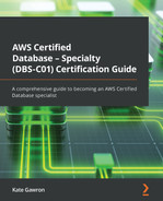
Amazon Neptune is deployed within a VPC. When it is deployed, you control access to it using subnetworks (subnets) and security groups. Neptune can be deployed as a cluster with Multi-AZ options, and its configuration is controlled using parameter groups in a similar manner to RDS instances. It is common to use Neptune in conjunction with other AWS services such as AWS Lambda (a serverless programming tool that allows you to run code without creating a server). A typical Neptune cluster across two Availability Zones (AZs) connecting these services can be seen in the following diagram:

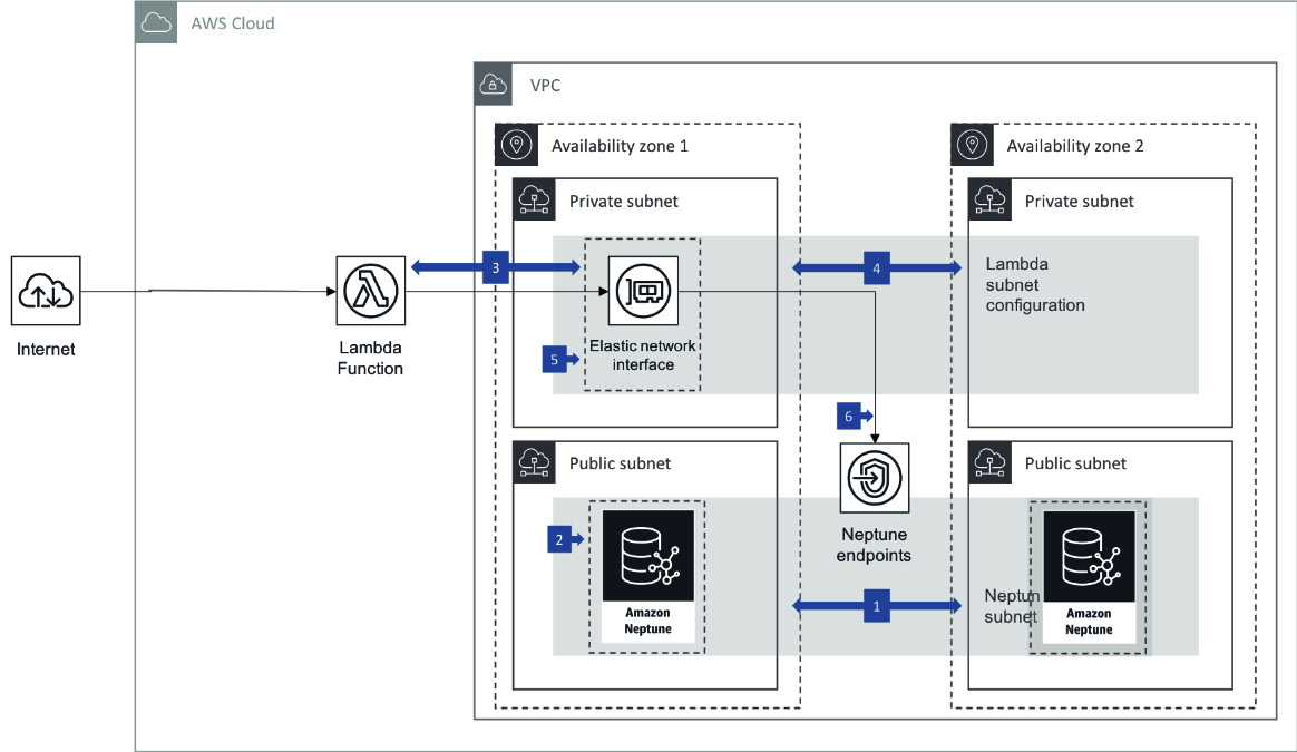
Figure 8.1 – Amazon Neptune Multi-AZ deployment with AWS Lambda

Amazon Neptune also supports cross-region replication using a service called Neptune Streams, which you can enable after you have created your Neptune cluster and copied a backup of your Neptune cluster across to the target region.

Now we've learned about Neptune topology and some key features, let's learn how to use Neptune data, including how to load and query data and how to work with graph data.

Working with Neptune

One of the first things to understand about graph databases is how they store data and, specifically, how Neptune stores data. Unlike RDBMS and some NoSQL systems (such as DynamoDB), graph databases do not use Structured Query Language (SQL) for querying. Instead, Neptune supports two different graph query languages: Gremlin and SPARQL Protocol and RDF Query Language (SPARQL). You can only use one language at a time in your database, and each language has its own requirements for how the data will be stored within Neptune and how you can utilize it. If you use Gremlin, the data stored will be using the Property Graph data framework, and if you choose SPARQL, you will be using the Resource Description Framework (RDF). SPARQL looks similar to SQL with SELECT and INSERT statements, but has some major differences with how it handles WHERE clauses and the syntax. Gremlin will appear unfamiliar to database administrators (DBAs) as it uses a structure more similar to programming languages such as Java or Python. Knowing the two different types of frameworks and languages you can use is important for the exam, but you will not need to know the specific differences between them.

Each item stored in Neptune consists of four elements, as outlined here:

• subject (S)—This can either refer to the name of the item or to the source item of a relationship (remember: graph databases focus closely on relationships, so they are defined specifically and stored, unlike in RDBMSs).
• predicate (P)—This describes the type of property that is being stored or the type of relationship. Consider this as a verb or a property description. Examples for relationships could be "likes," "bought," "owns" or, for a property of an item, "color," "name," or "person."
• object (O)—For a relationship, this will refer to the target item, and for a property, it will be the value you want to store.
• graph (G)—This is an optional parameter that can be used to create a named graph identifier (ID), or it can store an ID value for a relationship that's been created.

By using the preceding syntax, you can build up a diagram of items with properties such as descriptions of a person, as well as relationships to other items, such as books they own. The following diagram shows a simple representation of how that could look:

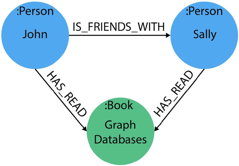
Figure 8.2 – Graph database showing people who have read a book

So, we now understand how Neptune stores data, but how do we load it? Let's look at how we can load data into a Neptune tool.

Loading data into Neptune

You can add data via SPARQL INSERT statements or their Gremlin equivalents, addE and addV. This approach would take a large amount of time for large datasets, and therefore Amazon offers the Neptune Bulk Loader. The Neptune Bulk Loader can read files hosted in a Simple Storage Service (S3) bucket and process them rapidly over the internal AWS network. The Neptune Bulk Loader tool takes advantage of endpoints (see Chapter 2, Understanding Database Fundamentals) to allow you to read and load data directly from an S3 bucket without having to open up your database subnets or security groups to the internet. It also allows you to use the AWS internal network, which operates at 10 gigabits per second (Gbps) and is often much faster than an AWS Direct Connect connection and faster than moving data via the public internet. You can also load data into Neptune using a tool called AWS Database Migration Service (DMS). DMS allows you to convert from an RDBMS database engine into Neptune. We will look at DMS in depth in Chapter 10, The AWS Schema Conversion Tool and AWS Database Migration Service.

Using Neptune Jupyter notebooks

One of the main use cases for using a graph database is the ability to quickly produce a graphical representation of your data. A graph database lends itself to producing a graphical model very quickly and easily because of how the data is stored; you don't need a complex data model to be able to see all the data connections as the connections themselves are stored as data items in the database. AWS offers a tool called Notebook that connects with Neptune and allows you to create graphs of your data rapidly. The notebooks use a framework called Jupyter, which is a graphical development environment designed for the web. You won't need to know any more about Jupyter for the exam.

Here is an example of how Neptune notebooks can visualize data based on your queries:

Figure 8.3 – Neptune notebook data visualization

The notebooks that are created run through another AWS service called Sagemaker. Sagemaker is a machine learning (ML) platform that is outside of the scope of the exam, but there may be a question on Neptune that mentions Sagemaker notebooks.

We've learned some of the key features of Neptune, how to load data, and how to query the data in a visual way, but how do you manage it? Let's look at that now.

Managing a Neptune cluster

Neptune is a fully managed database system, meaning that patching and backups are handled by AWS within the maintenance window and backup retention policies you set. However, areas such as instance sizing and read replicas remain under your control.

A Neptune instance can have up to 15 read replicas within the same region to allow you to scale your cluster horizontally. You can also change the instance class of both your primary database and read replicas at any time to make sure they are appropriately sized for your workload. Neptune supports auto-scaling of read replicas via an auto-scaling group, but it does not support auto-scaling of the instance class—this must be changed manually. Neptune sends logs by default to CloudWatch, allowing you to monitor its performance closely. CloudWatch also allows you to set up alarms against specific metrics to warn you if a cluster needs to be modified to handle a larger-than-expected workload.

Neptune will automatically scale your storage as your database grows, up to a maximum of 64 tebibytes (TiB). When it is first provisioned, you are given 10 gigabytes (GB) of storage, which will automatically grow as needed. Storage will not automatically shrink if data is deleted, but the Neptune database will instead try to optimize the storage. As the storage grows, Neptune updates the high-water mark (HWM). The HWM is the value used to calculate your storage costs. Neptune makes size copies of your data, but you are only charged for one, so if your database reaches 100 GB in size, you are only billed for 100 GB and not 600 GB as you may expect, given there are six copies of your data (two copies in three different AZs). If you wish to reduce the storage size and reduce your storage costs, you need to export the data from the database and import it into a new Neptune database; you cannot do this in situ.

Neptune uses parameter groups to control the configuration of a Neptune cluster. There are two types of parameter groups: database and cluster. Database groups allow you to set different parameters for each database, but cluster groups will affect all databases, including read replicas. You can override a cluster group parameter by modifying the database group last, as the latest changes take precedence.

We've now learned the main features of an Amazon Neptune database and cluster, including how to load data. Now, let's deploy a Neptune cluster and load some data into it.

Deploying a Neptune cluster

The first step we are going to do is to create a single, standalone Neptune cluster. Once the cluster is provisioned, we will load some data and install and configure a Gremlin client to allow us to query the data in the database.

Note

Neptune is not included in the AWS free tier, so following this lab will be chargeable by AWS. This lab is designed to keep costs at a minimum while learning the critical elements required for the exam.

Let's start by creating our Amazon Neptune cluster, as follows:

1. Log in to the AWS console and navigate to Neptune.
2. Click Launch Amazon Neptune, as illustrated in the following screenshot:

Figure 8.4 – Launch Amazon Neptune

3. Complete the Create database form, as follows. If a value is not mentioned, please leave it as its default:
   • Settings | DB cluster identifier: dbcert-neptune
   • Templates: Development and Testing
   • DB instance size | DB instance class: db.t3.medium
   • Connectivity | Virtual Private Cloud (VPC): Select the VPC you created in Chapter 2, Understanding AWS Fundamentals
   • Connectivity | Additional connectivity configuration|VPC security group: Create a new one and enter dbcert-neptune-sg
   • Notebook configuration: Uncheck Create notebook
   • Additional configuration—Log exports: Uncheck Audit log
4. Click Create database. The database will take around 10 minutes to show an Available status, which you can see in the following screenshot:

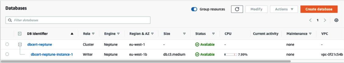
Figure 8.5 – Neptune dashboard screen

5. You will be able to see the cluster and a single Writer node.

Now we have our Neptune database up and running, we will load some data and run some queries. We'll start by loading data into an S3 bucket and granting Neptune read permissions. Proceed as follows:

1. Navigate to the https://github.com/PacktPublishing/AWS-Certified-Database---Specialty-DBS-C01-Certification/tree/main/ch8 GitHub Uniform Resource Locator (URL) and download two files, airports.csv and flight_routes.csv.
2. Return to the AWS console and navigate to S3.
3. Click Create bucket on the right-hand side, as illustrated in the following screenshot:

Figure 8.6 – Creating an S3 bucket

4. Complete the Create bucket form, as follows. Leave any values not mentioned as default:
   • General configuration|Bucket name: dbcert-s3-<your name>. S3 buckets must have unique names globally.
   • General configuration|AWS Region: EU (Ireland) eu-west-1.
5. Click Create bucket.
6. Click the bucket name you just created from the dashboard and select Upload, as illustrated in the following screenshot:

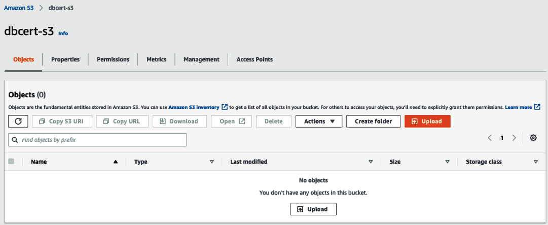
Figure 8.7 – S3 bucket upload

7. Locate the two .csv files you downloaded and upload those into the bucket, as illustrated in the following screenshot:

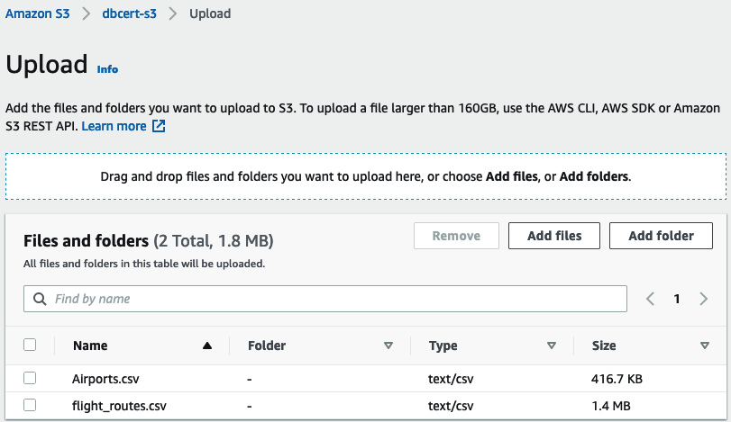
Figure 8.8 – S3 upload files

8. Click Upload at the bottom and wait for the transfer to complete. It will take around a minute on a standard internet connection. Wait until both files show as Succeeded.

We now need to create an S3 endpoint so that Neptune can access the data in the bucket. Proceed as follows:

1. Navigate to VPC service in the AWS console.
2. In the left navigation pane, choose Endpoints.
3. Click Create Endpoint.
4. Enter s3 in the search bar and select com.amazonaws.eu-west-1.s3 for the Service name value. Choose a value for Gateway type.
5. Choose the VPC that contains your Neptune database instance.
6. Select the checkbox next to the route tables that are associated with the subnets related to your Neptune database cluster. If you only have one route table, you must select that box.
7. If you wish, review the policy statement that defines this endpoint.
8. Click Create Endpoint.
9. An endpoint will be created immediately and you will see it in the dashboard view, as illustrated in the following screenshot:

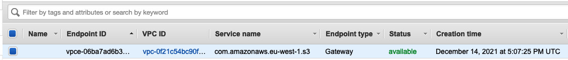
Figure 8.9 – Endpoint dashboard

The next step is to set up identity and access management (IAM) roles to allow the Neptune instance to communicate with the S3 bucket. Proceed as follows:

1. Log in to the AWS console and navigate to IAM.
2. Click Roles from the menu and then select Create role.
3. Click the AWS service button and then select S3 from the list, as illustrated in the following screenshot. Select S3 again in the Select your use case option at the bottom, and then click Next: Permissions:

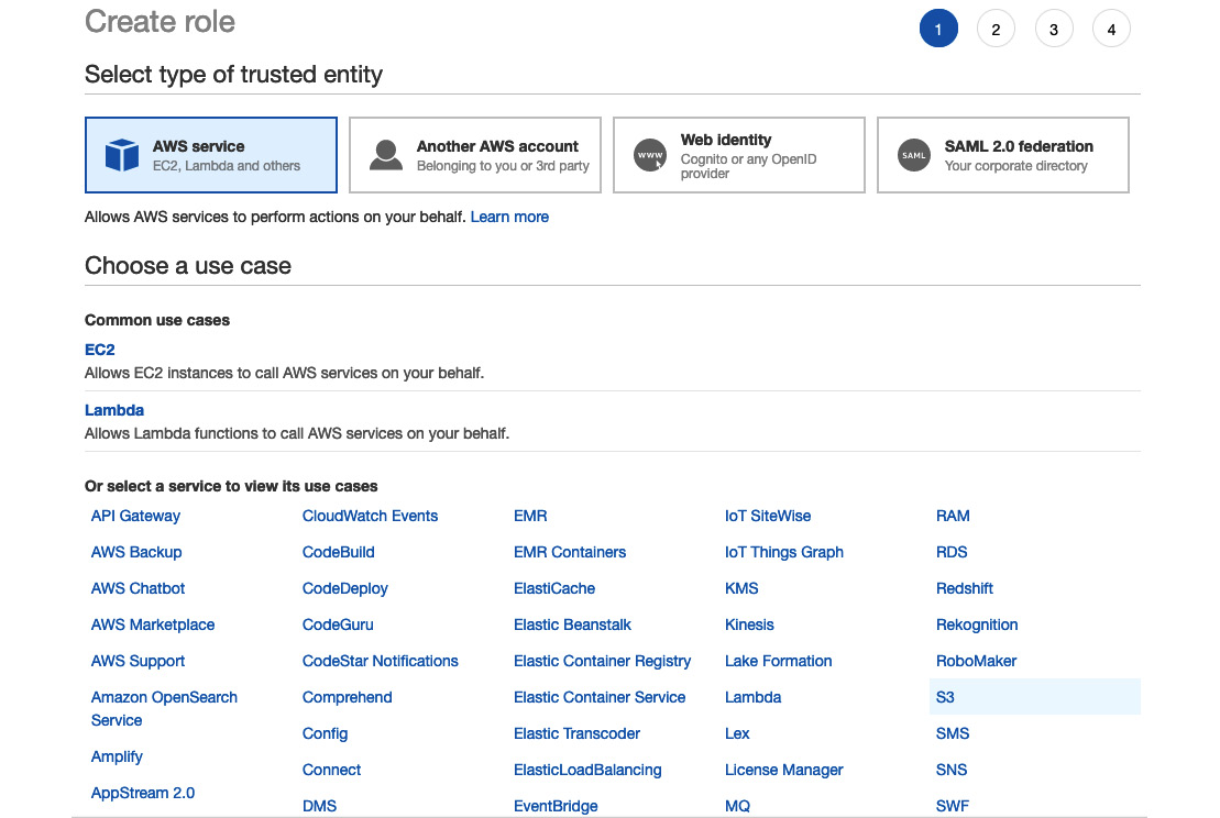
Figure 8.10 – Selecting the S3 service

4. Enter AmazonS3ReadOnlyAccess in the search box and then check the checkbox in the table below, as illustrated in the following screenshot. Then, click Next: Tags:

Figure 8.11 – Adding role permissions

5. Click Review.
6. Enter a name for the role, such as dbcert-neptune-s3, and click Create role.
7. Once the role has been created, click Roles from the left-hand menu and enter the name of the role you just created in the search box. Click the role name you created.
8. Click the Trust relationships tab, as illustrated in the following screenshot:

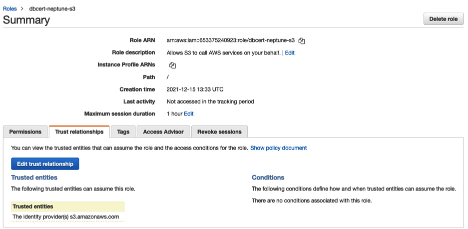
Figure 8.12 – Adding a trust relationship

9. Click Edit trust relationship and replace the code with the following code:

   {

     "Version": "2012-10-17",

     "Statement": [

       {

         "Sid": "",

         "Effect": "Allow",

         "Principal": {

           "Service": [

             "rds.amazonaws.com"

           ]

         },

         "Action": "sts:AssumeRole"

       }

     ]

   }

This code allows an RDS instance (of which Neptune is classified) to use this role.

10. Click Update trust policy.
11. Make a note of the Role ARN value, as shown in the following screenshot, as we will need it later on:

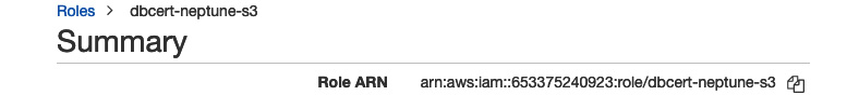
Figure 8.13 - Making a note of the Role ARN value

12. Navigate to Neptune from the AWS console.
13. Select the database with the cluster role you created earlier, and then select Manage IAM roles from the Actions dropdown, as illustrated in the following screenshot:

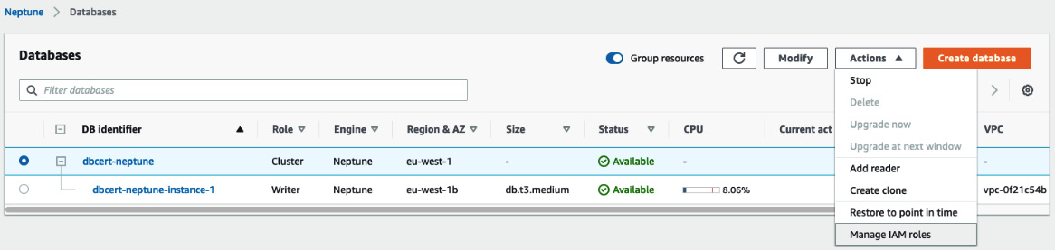
Figure 8.14 – Assigning the IAM role to Neptune

14. Select the role you just created and click Done.

We will now create an Elastic Compute Cloud (EC2) instance from which we can run commands against the Neptune database. Proceed as follows:

1. Log in to the AWS console and navigate to EC2.
2. Click Launch instance from the EC2 dashboard.
3. Select Amazon Linux 2 AMI, as illustrated in the following screenshot. Any kernel version is fine. Your Amazon Machine Image (AMI) details will vary depending on the region you choose:

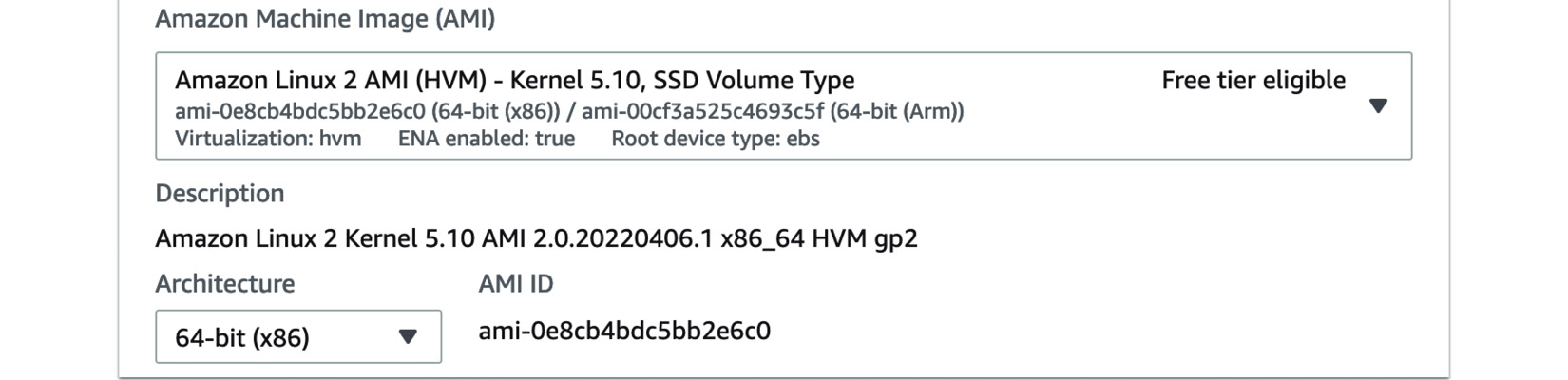
Figure 8.15 - The Elastic Compute Cloud dashboard

4. Choose t2.micro, which is part of the free tier, as illustrated in the following screenshot:

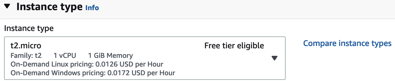
Figure 8.16 – Choosing the right EC2 instance size

5. Click Next: Configure Instance Details.

Under Network, select the same VPC that the Neptune database was launched in. The VPC we built in Chapter 2, Understanding Database Fundamentals, will meet the requirements. Select any public subnet from the Subnet dropdown, as illustrated in the following screenshot—you can tell if it's a public subnet if the Auto-assign Public IP default value is (Enable). This is important so that we can connect to this EC2 instance. Leave all other values as default and click Review and Launch:

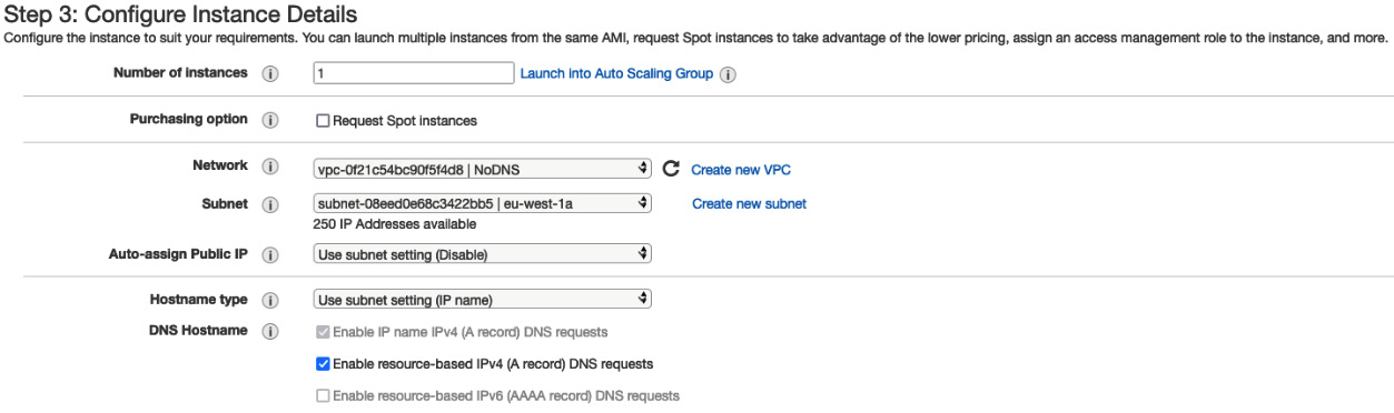
Figure 8.17 – EC2 launch configuration

6. On the Review Instance Launch page, click Edit security groups.
7. Create a new security group called dbcert_neptune_ec2_sg. Edit the rule to allow Secure Shell (SSH) on port 22 from your Internet Protocol (IP) address. This is so that we will be able to access the instance. The process is illustrated in the following screenshot:

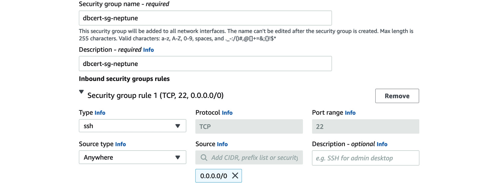
Figure 8.18 – Security group configuration

8. Click Review and Launch and then click Launch.
9. Select Create a new key pair from the dropdown and enter a name, such as dbcert-neptune-kp. Click Download Key Pair and then Launch Instances.
10. Return to the EC2 Dashboard and wait for the Instance State value to show as Running. This will take a few minutes.
11. We now need to add a rule to our Neptune database cluster security to allow the EC2 instance to connect to it. Navigate to the VPC service from the console main menu.
12. Select Security groups from the left-hand menu and locate your Neptune security group, which we called dbcert_neptune_sg.
13. Add a rule to allow dbcert_neptune_ec2_sg to connect to it on port 8182.

Once the instance is running, we will try to connect to it using the EC2 instance connect tool. You can also try to use an ssh command from your local computer, but this is beyond the scope of this lab. Proceed as follows:

1. Select the instance you just created, and then click Connect.
2. Select EC2 Instance Connect and leave the username as ec2-user, as illustrated in the following screenshot:

Figure 8.19 – Connecting to an EC2 instance

3. Click Connect.

A screen similar to this should appear:

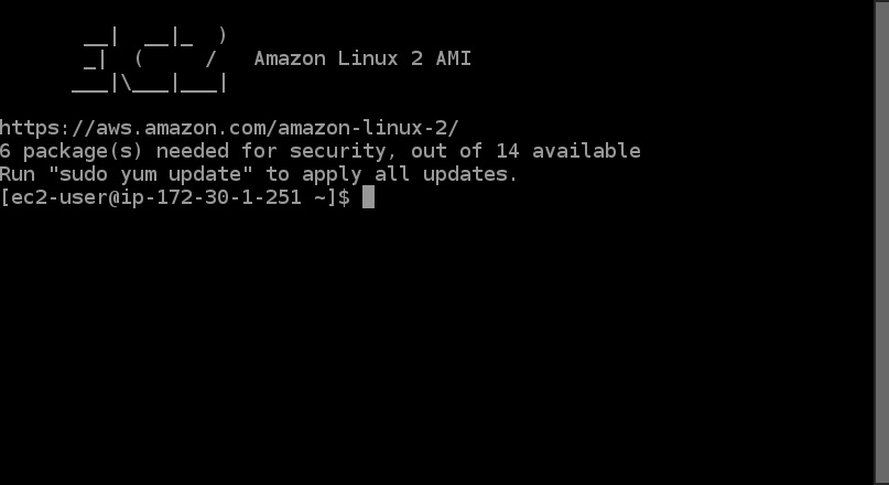
Figure 8.20 – EC2 terminal

We are now going to use a tool called curl that allows to you run commands using HyperText Transfer Protocol (HTTP). You won't need to know about curl beyond this lab for the exam, but there is a recommendation in the Further reading section if you wish to know more.

4. In a different browser window or tab, navigate to the Neptune dashboard.
5. Click on the Writer node and make a note of the Endpoint and Port values under the Connectivity & security tab.
6. Return to your EC2 session and run the following curl command. You will need to modify the sections highlighted to match your own values:

   curl -X POST

       -H 'Content-Type: application/json'

       https://dbcert-neptune-instance-1.cdhcmbt6wawh.eu-west-1.neptune.amazonaws.com:8182/loader -d '

       {

         "source" : "s3://dbcert-s3-kgawron",

         "format" : "csv",

         "iamRoleArn" : "arn:aws:iam::653375240923:role/dbcert-neptune-s3",

         "region" : "eu-west-1",

         "failOnError" : "FALSE",

         "parallelism" : "MEDIUM",

         "updateSingleCardinalityProperties" : "FALSE",

         "queueRequest" : "FALSE"

       }'

You will get the following output, showing the import is running:

{

    "status" : "200 OK",

    "payload" : {

        "loadId" : "03edf947-9702-48f5-8fa3-e2f1f31ba749"

    }

Now we have some data in the database, we need to install Gremlin to be able to run it.

7. From your EC2 instance, install Java, like so:

   sudo yum install java-1.8.0-devel

8. Now, download and install the Gremlin console, as follows:

   wget https://archive.apache.org/dist/tinkerpop/3.4.8/apache-tinkerpop-gremlin-console-3.4.8-bin.zip

   unzip apache-tinkerpop-gremlin-console-3.4.8-bin.zip

9. Change directory to apache-tinkerpop-gremlin-console-3.4.8.
10. Download and install Amazon certificates. Neptune uses a Secure Sockets Layer (SSL) connect, so to connect to it, we need an SSL certificate. Change the Java location to match the one you have downloaded. The code is illustrated in the following snippet:

    wget https://www.amazontrust.com/repository/SFSRootCAG2.cer

    mkdir /tmp/certs/

    cp /usr/lib/jvm/java-1.8.0-openjdk-1.8.0.312.b07-1.amzn2.0.1.x86_64/jre/lib/security/cacerts /tmp/certs/cacerts

    sudo keytool -importcert

                 -alias neptune-tests-ca

                 -keystore /tmp/certs/cacerts

                 -file  /home/ec2-user/apache-tinkerpop-gremlin-console-3.4.8/SFSRootCAG2.cer

                 -noprompt

                     -storepass changeit

11. Change into the conf directory and create a file called neptune-con.yaml with the following contents. You will need to change the values highlighted to match your own Neptune database. [] brackets are needed:

    hosts: [dbcert-neptune.cluster-cdhcmbt6wawh.eu-west-1.neptune.amazonaws.com]

    port: 8182

    connectionPool: { enableSsl: true,  trustStore: /tmp/certs/cacerts }

    serializer: { className: org.apache.tinkerpop.gremlin.driver.ser.GryoMessageSerializerV3d0, config: { serializeResultToString: true }}

12. Go back to the apache-tinkerpop-gremlin-console-3.4.8 directory and run bin/gremlin.sh. This will load the Gremlin console.
13. At the gremlin> prompt, enter the following code to load your Neptune configuration and then tell Gremlin to use it:

    :remote connect tinkerpop.server conf/neptune-con.yaml

    :remote console

14. We can now run Gremlin queries, such as finding out how many components there are, as follows:

    g.V().label().groupCount()

Or, we can find out where we can fly direct to from London Heathrow, as in this example:

g.V().has('code','LHR').out().path().by('code')

Feel free to review the Further reading section, which has a guide on more detailed Gremlin queries if you wish. When you are finished, type :exit to quit the Gremlin console.

15. You can now clear up the environment, including the EC2 instance you created.

Now we've learned about Neptune and have completed a hands-on lab covering all the topics that may come up in the exam, let's learn about another purpose-built database offered by AWS—QLDB.

Overview of Amazon QLDB

Amazon QLDB is a fully managed, transparent, immutable, and cryptographically verifiable transaction log database. What does this really mean? If you consider running an UPDATE or DELETE statement against a typical RDBMS, what happens? If you have logging enabled, then that transaction should be stored in the logs, but there will be no record of the change within the database. It would be fairly simple for someone to make changes and for those logs to be deleted or lost (how long are transaction logs kept for before being deleted?), and then all record of that change is also lost. QLDB not only stores the latest version of a record after it's been updated or deleted but also stores all the previous versions within the database itself. Additionally, the database ensures that every new version of a record contains an algorithmic reference to the previous version, meaning that any attempt to modify a record without making a record of the change will cause the algorithm to fail, and hence alert that someone has tampered with the system. As a result, QLDB is the perfect database to use when you need to have absolute guarantees over the accuracy of data; use cases such as financial transactions or medical cases are commonly cited when considering QLDB.

A QLDB table will look similar to this:

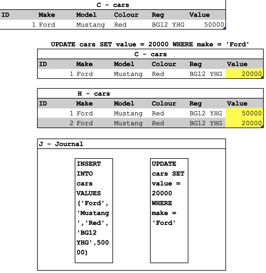
Figure 8.21 – QLDB schema view

The C table holds the current state of a record, the H table holds all the historical values that the record had, and the J table holds a log of all changes that have been made. The J table contains what are called digests. These are alphanumeric strings known as a hashchain. A hashchain is added to every time a record is amended. Each new entry contains all the previous entries, so the values grow as the database changes. As each entry contains all the previous entries too, any entry to the journal must match; otherwise, the change will be seen by the database and the verification will fail. Changing any data in the database without it being tracked requires every journal entry for that record to also be changed at the same time. This would require computing power that doesn't currently exist, therefore a QLDB instance is classed as immutable and cryptographically verifiable. You can query any of three tables at any time, depending on the data you require.

Let's take a look at the QLDB architecture and how you deploy it within AWS.

QLDB architecture

QLDB is deployed by default across multiple AZs, with multiple copies of the data also being stored in each AZ. This makes it both resilient to a software failure and fast to recover from and durable if storage is lost. A write to QLDB is only committed once the data has been successfully written to multiple storage locations in more than one AZ.

QLDB is a serverless database. This means that you do not need to provision compute capacity or storage amounts for it as it will auto-scale seamlessly with demand.

One of the main benefits of QLDB is its interconnectivity with other AWS services. You can quickly and easily connect QLDB to tools such as Amazon Kinesis Data Streams, which monitors the logs of the database and takes actions based on them. For example, you can configure Amazon Kinesis to forward all data modifications to an RDS instance. Due to how QLDB manages the data, it can be much slower to query than an equivalent non-immutable database in RDS, so connecting the two systems together in this way would allow you to run faster read-only queries against the RDS system, but have an immutable copy of the data stored in QLDB for verification purposes. Here is an example of that architecture, whereby QLDB is used for all writes, and reads are from an Aurora RDS database:

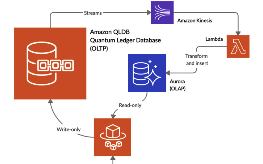
Figure 8.22 – QLDB and Aurora architecture example

Now we've learned how Amazon QLDB works and is provisioned, let's look at how you access and query it.

Accessing a QLDB database

QLDB has three methods to query data, as follows:

• AWS console—QLDB has a built-in graphical query tool.
• Amazon QLDB shell—You can use a downloadable shell and connect from your local machine to the QLDB instance and run queries.
• AWS application programming interface (API)—You can download a QLDB driver and make calls to the QLDB instance using a variety of coding languages such as Java, .NET, and Python.

These methods all use a language called PartiQL (pronounced particle) to run queries. PartiQL uses a similar structure to SQL queries, allowing you to run SELECT, UPDATE, and DELETE statements complete with WHERE clauses. Here's an example of this:

SELECT * FROM Cars AS c WHERE c.Reg IN ('BG12 YHG', 'D150 GWE');

Here is the output for the previous query. It follows a syntax called Amazon Ion, which closely resembles JavaScript Object Notation (JSON) syntax:

{

    Make: "Ford",

    Model: "Mustang",

    Color: "Red",

    Reg: "BG12 YHG",

    Value: 20000

}

You can use PartiQL for joining tables, doing aggregation queries (for example, MAX or AVG). You can also use PartiQL to obtain the metadata of a record. Metadata refers to information about the record itself rather than the data within it. Metadata might include the RecordID value, the date it was added or modified, or the size of the record. QLDB allows you to query this metadata by querying system tables. For example, to obtain all the metadata and data for the latest committed version of a specific record, you can use this query (note the addition of _ql_committed_ to the table name):

SELECT * FROM _ql_committed_Cars AS c WHERE c.Reg IN ('BG12 YHG', 'D150 GWE');

This query will return the hash value for that record as well as its version number (the number of times it's been updated since first inserted) and the block address (which is the physical location on the storage). It also returns a metadata ID value, which can be used to query historic versions of that record. This is an example output you would see:

{

    blockAddress:{

        strandId:" 5PLf9SXwndd63lPaSIa0O6",

        sequenceNo:9

    },

    hash:{{LuCf20C1fBB0s7HRV5m28FSxlxn94Z9o3FbePOCF8WO=}},

    data:{

        Make: "Ford",

    Model: "Mustang",

    Color: "Red",

    Reg: "BG12 YHG",

    Value: 20000

    },

    metadata:{

        id:"QgSrP4SPSwUWI0RjxureT3",

        version:0,

        txTime:2021-12-08T11:15:261d-3Z,

        txId:"KaYBkLjAtV0HQ4lNYdzX60"

    }

}

As QLDB stores the details of all changes made in the history table, you can write a query to see all previous values of a record or limit it to a time range, as in the following example:

SELECT * FROM history(Cars, `2021-12-07T00:00:00Z`, `2021-12-10T23:59:59Z`) AS h WHERE h.metadata.id = 'QgSrP4SPSwUWI0RjxureT3'

The output would show you all changes made between those dates, as illustrated here:

{

    blockAddress:{

        strandId:" 5PLf9SXwndd63lPaSIa0O6",

        sequenceNo:9

    },

    hash:{{LuCf20C1fBB0s7HRV5m28FSxlxn94Z9o3FbePOCF8WO=}},

    data:{

      ...

      Value: 50000

    },

    metadata:{

        id:"QgSrP4SPSwUWI0RjxureT3",

        version:0,

        txTime:2021-12-08T08:43:321d-3Z,

        txId:"KaYBkLjAtV0HQ4lNYdzX60"

    }

},

{

    blockAddress:{

        strandId:" 5PLf9SXwndd63lPaSIa0O6",

        sequenceNo:12

    },

    hash:{{Qleu1L9OQuqvZP57n9nw5aCqNrIDW7ywAb8QX1ps1Rx =}},

    data:{

      ...

      Value: 20000

    },

    metadata:{

        id:"QgSrP4SPSwUWI0RjxureT3",

        version:1,

        txTime:2021-12-08T11:15:261d-3Z,

        txId:" 7nGrhIQV5xf5Tf5vtsPwPq"

    }

}

Note how the txId (transaction ID) value changes, but not the metadata ID value. The version number increases with every change, with version 0 being the first committed version.

Quotas and limits for QLDB

QLDB has some limits you may need to be aware of for the exam. The key ones are noted here:

• Number of active ledgers in any one region—5
• Maximum concurrent session in any one ledger—1,500
• Maximum number of active tables—20
• Maximum number of tables active or inactive (dropped tables are called inactive, so count toward this limit)—40
• Maximum document size—128 kilobytes (KB)

Now we've learned how to access and query QLDB and found out about some of the limits that may come up in the exam, let's put our knowledge to use in a hands-on lab, deploying a QLDB ledger.

Deploying a QLDB database

Let's now use the AWS console to deploy, load data into, and query a QLDB database. First, we will create our ledger.

Note

QLDB is not included in the AWS free tier, so following this lab will be chargeable by AWS. This lab is designed to keep costs at a minimum while learning the critical elements required for the exam.

Proceed as follows:

1. Go to the AWS console and navigate to Amazon QLDB.
2. Click Create ledger.
3. Enter dbcert-qldb as a value for Ledger name and leave all other values at their default settings. Click Create ledger at the bottom of the page.
4. The database will take a few minutes to create, so wait until the Status column shows as Available.

Now, we need to load data into our ledger. We will use sample data provided by AWS for testing.

5. Click on Getting started from the menu on the left-hand side and scroll down until you find the Sample application data section, as illustrated in the following screenshot:

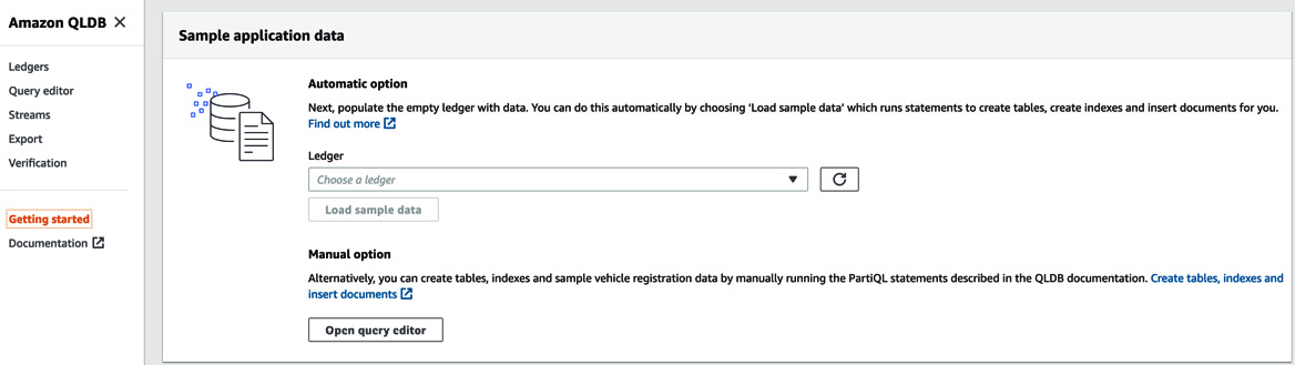
Figure 8.23 – Loading sample data

Select your ledger from the dropdown and click Load sample data.

6. Once the data has loaded click Query editor on the left-hand menu
7. Select your ledger from the dropdown and wait for a list of tables to be loaded.
8. Click on the table names to view indexes from which you can build your queries. Type the following command into the query window and then click Run:

   select VIN from Vehicle

You will receive the following output:

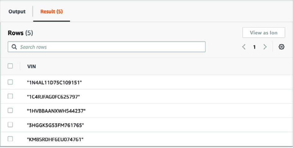
Figure 8.24 – Query output

9. Experiment with different queries against _ql_committed_ tables, as follows:

   select * from _ql_committed_Vehicle

10. When you are finished, you can delete the QLDB ledger. You will need to modify the ledger to remove Deletion protection before you can do so.

We've now learned all the key features you will need to know on QLDB for the exam. Let's now learn about the final purpose-built database AWS offers: Amazon Timestream.

Overview of Amazon Timestream

Amazon Timestream is a time-series database. A time-series database is optimized for storing and querying data saved in key pairs of time and value. It is often used when data is being stored from sensors or operations with a timestamp and associated value that need to be tracked for trending analysis.

Timestream is a fully-managed, serverless, and scalable database service specifically customized and optimized for Internet of Things (IOT) devices and application sensors, allowing you to store trillions of events per day up to 1,000 times faster than via an RDBMS. Being serverless means you do not need to define your compute values, as Timestream will automatically scale up and down depending on the current workload.

Timestream features a tier-storage solution that moves older and less frequently accessed data to a cheaper storage tier, saving costs. Timestream has its own adaptive query engine that learns your data access patterns to optimize query retrieval speed and can access all the different storage tiers at the same time, making querying simpler and more efficient. Timestream also auto-scales your storage so that you do not need to pre-allocate storage space, as Timestream will grow the storage as required.

Let's look at Timestream architecture and how it differs from other databases.

Timestream architecture

Timestream features two main components: an in-memory data store for fast writes and reads, and a permanent data storage layer for redundancy and resilience. The following diagram shows the architecture used:

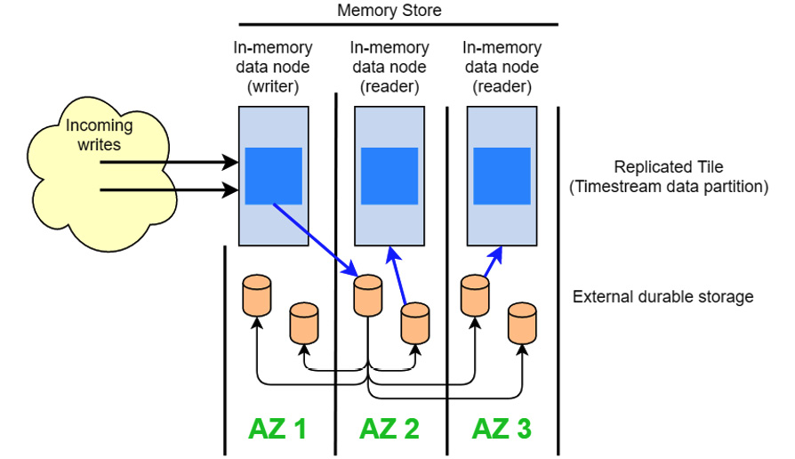
Figure 8.25 – Timestream architecture

Timestream will automatically move data from the memory store to the durable storage based on lifecycle policies you can set. For example, you can tell Timestream to move any data older than 24 hours to durable storage. Data being read from durable storage will be much slower than from memory, but storing in memory is more expensive. Managing lifecycle policies correctly will allow you to handle most queries from data held in the fast memory store while not holding rarely queried data, thereby increasing your costs.

Timestream does not require you to create a schema before using it. Timestream will automatically create tables for you based on the dimensions and attributes you ask it to store. Here is an example of a Timestream table:

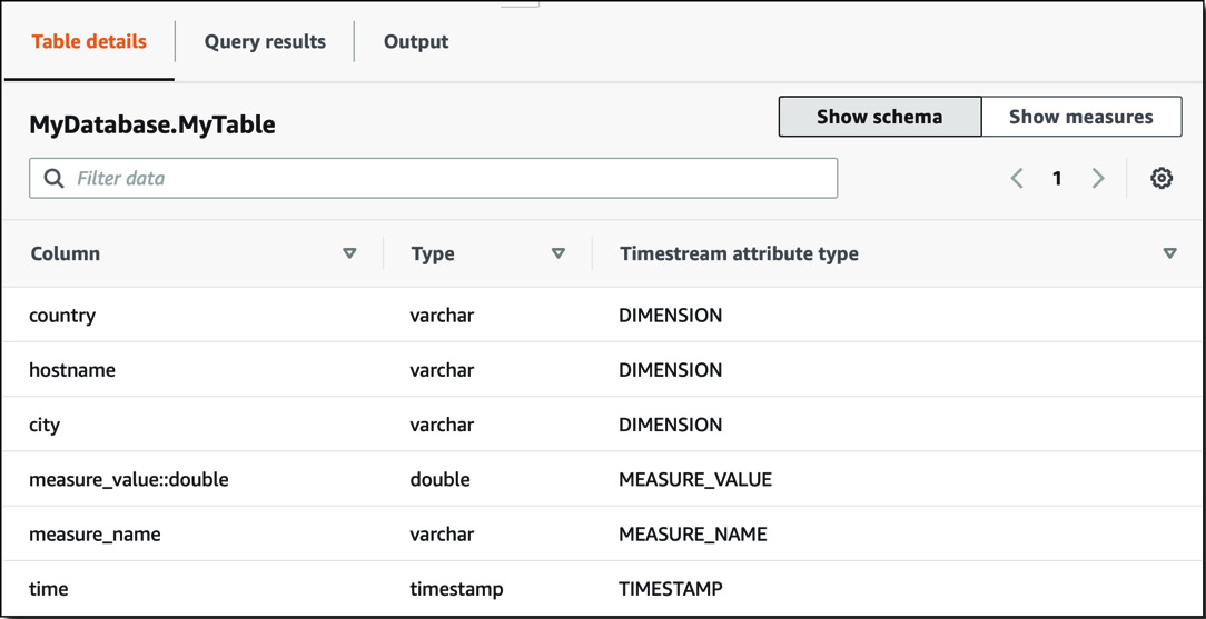
Figure 8.26 – Timestream schema

You can see column names, types, and the Timestream attribute type. The Timestream attribute type will be one of four, as outlined here:

• DIMENSION—This is metadata about the entry and contains extra information about the data that is being stored.
• MEASURE_NAME—This is the name of the measure that is being taken. This could be something such as weight, size, speed, and so on.
• MEASURE_VALUE—This is the value that has been measured.
• TIMESTAMP—This is the time the value was taken.

This is an example of how data could look using that schema:

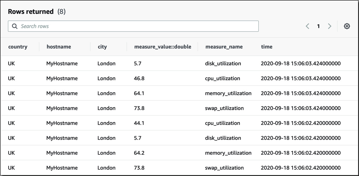
Figure 8.27 – Timestream query

Timestream stores data in time order sorted by dimensions. For example, in the previous query, the data would be first organized by country, hostname, and city, and then it would be sorted in timestamp order. As most queries will contain a WHERE clause filtering on one or more dimension values, this will ensure the highest performance as all of those values will be located together in the same memory or durable storage area, allowing them to be returned simultaneously without multiple disk reads.

Timestream natively supports the forwarding of data to other AWS services vis Amazon Kinesis. It is common for Timestream to be connected to graphically querying tools such as Amazon QuickSight or Grafana to use visualization to aid trending and analysis.

We've learned about the high-level architecture and schema design of a Timestream database, but how do we query it and load data? Let's learn how to do that now.

Accessing a Timestream database

Timestream can be queried using three different methods, as follows:

• AWS console—Timestream has a built-in graphical query tool.
• AWS CLI—You can use the AWS CLI to run both write and read queries from your local computer.
• AWS API/software development kit (SDK)—You can download a Java Database Connectivity (JDBC) driver and make calls to Timestream using a variety of coding languages such as Java, .NET, and Python.

Timestream supports queries written in SQL, allowing you to run SELECT and INSERT statements combined with WHERE clauses to filter. You cannot run a DELETE statement from Timestream, nor run an UPDATE statement against an existing entry, as this will break the time pattern. You can also run a scheduled query. Given the time-sensitive nature of Timestream use cases, it's common to create daily or weekly reports showing trends, patterns, and exceptions. Scheduled queries are used to create views that can then in turn be queried. This can greatly improve the performance of your queries as the aggregated data has already been collated, and therefore you are only querying against a subset held in memory. A typical use case for scheduled queries is to connect an ML tool such as AWS SageMaker to identify exceptions that may point to fraud or sensor failure.

Loading data into Timestream

Timestream doesn't have any method to bulk-load data as it is designed to receive a large amount of data from sensors in real time rather than as a bulk data load. You can import a sample dataset for testing when you deploy Timestream.

Let's do that now—we'll learn how to deploy a Timestream database, import some sample data, and then run some queries.

Deploying a Timestream database

Let's now use the AWS console to deploy, load data into, and query a Timestream database. First, we will create our table.

Note

Timestream is not included in the AWS free tier, so following this lab will be chargeable by AWS. This lab is designed to keep costs at a minimum while learning the critical elements required for the exam.

Proceed as follows:

1. Go to the AWS console and navigate to Amazon Timestream.
2. Click Create database.
3. Choose Sample database. Enter dbcert-timestream as the Database name value and leave all other values at their default values. Click Create database at the bottom of the page.
4. A database will take be created immediately, complete with sample data loaded.
5. Click Query editor on the left-hand menu.
6. Select your database from the dropdown and wait for a list of tables to be loaded.
7. Click on the table names to view columns from which you can build your queries. Type the following command into the query window and then click Run:

   select truck_id from "dbcert-timestream.IotMulti"

You will receive the following output:

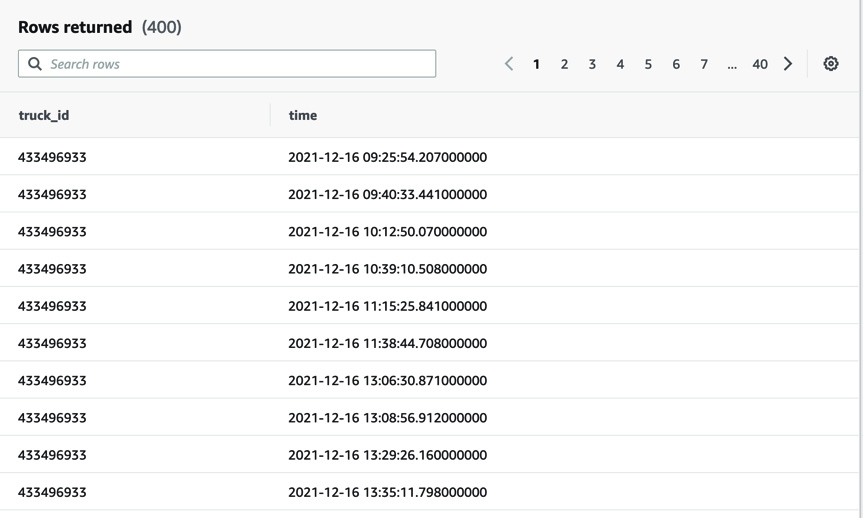
Figure 8.28 – Timestream query output

You can see many entries for the same truck_id value. This data isn't very useful, so let's add some aggregation to the query, as follows:

SELECT truck_id, fleet, fuel_capacity, model, load_capacity, make, measure_name FROM "dbcert-timestream".IoTMulti GROUP BY truck_id, fleet, fuel_capacity, model, load_capacity, make, measure_name

8. Experiment with different queries. Sample queries are accessible via the Sample queries tab. Make sure you only select IoTMulti queries, else you will receive an error.
9. When you are finished, you can delete the Timestream database. You will need to delete the tables before you can delete the database. You can delete tables from the Tables option on the left-hand side of the screen.

We've now learned all the key features of Amazon Timestream, as well as how to deploy and query a Timestream database.

This completes our learning around the different databases offered by AWS that you will need to know for the exam. Let's now review our learning from this chapter.

Summary

In this chapter, we have learned about the final three new databases offered by AWS: Neptune, QLDB, and Timestream. We have learned that Neptune is a graph database fully managed by AWS and is used to define connections between records. We also learned how to use Gremlin and the Neptune Bulk Loader to query and load data.

For QLDB, we discovered what immutable means and how QLDB stores data and all historical versions, making it impossible for it to be changed without leaving a record.

Finally, we learned how to store large amounts of time-value data in Timestream that optimizes storage and queries of data from sensors or IoT devices.

We have now learned about all the different databases that AWS offers and that are covered in the exam. We have practiced working with the AWS console and the AWS CLI to create, query, and delete the databases. We have also learned how to work with other AWS services such as S3 and IAM.

In the next chapter, we are going to learn about how to use two database migration tools offered by AWS: Schema Conversion Tool (SCT) and Database Migration Service (DMS).

Let's now review the key points of this chapter in the Cheat sheet section.

Cheat sheet

This cheat sheet summarizes the main key points from this chapter, as follows:

• Neptune is a graph database optimized for storing and querying connections between items.
• You can use the Neptune Bulk Loader to import data in various formats from an S3 bucket using S3 endpoints.
• Neptune supports querying using the SPARQL language, which is similar to SQL, as well as Gremlin, which is a specific graph querying language.
• Neptune is a highly redundant, fully managed database system with options for both Multi-AZ and cross-region replication using Neptune Streams.
• QLDB is an immutable centralized ledger database optimized for workloads that require verifiable data chains with all historic versions and modifications.
• QLDB uses the PartiQL query language and returns data in Amazon ION format.
• QLDB does not offer any backup or restore functionality, but you can export to S3.
• QLDB scales automatically, so you do not need to provision compute or storage for it.
• Timestream is a fully managed, scalable database service optimized for time-series data, typically from sensors or IoT devices.
• Timestream creates a schema for you dependent on the data you load, so it allows for fully customized tables created at runtime.
• Timestream offers data management policies to store data on cheaper magnetic storage for less frequently accessed data, while frequently accessed data is stored with memory for rapid querying.
• Timestream supports querying using SQL syntax, allowing for complex aggregated queries.

Review

Let's now review your knowledge with this quiz:

1. You are working as a database consultant for a health insurance company. You are constructing a new Amazon Neptune database cluster, and you try to load data from Amazon S3 using the Neptune Bulk Loader from an EC2 instance in the same VPC as the Neptune database, but you receive the following error message: Unable to establish a connection to the s3 endpoint. The source URL is s3://dbcert-neptune/ and the region code is us-east-1. Kindly confirm your S3 configuration.

Which of the following activities should you take to resolve the issue? (Select two)

1. Check that a Neptune VPC endpoint exists.
2. Check that an Amazon S3 VPC endpoint exists.
3. Check that Amazon EC2 has an IAM role granting read access to Amazon S3.
4. Check that Neptune has an IAM role granting read access to Amazon S3.
5. Check that Amazon S3 has an IAM role granting read access to Neptune.

2. You are working with an Amazon Timestream database and are trying to delete records that have been loaded incorrectly. When running the DELETE FROM "dbcert-timestream"."test-table" statement, you receive the following error: The query syntax is invalid at line 1:1.

What is the most likely reason for the error?

1. The quotes are wrong in the SQL statement
2. The table name is incorrect
3. You cannot run a DELETE statement on a Timestream database
4. You do not have the correct IAM permissions

3. You are a DBA for a large financial company that is exploring QLDB. You have created a QLDB with 20 tables and are trying to create another one via the QLDB shell when you receive an error.

What is the most likely cause?

1. Someone has dropped the ledger you were working on.
2. The QLDB service is currently unavailable.
3. There are too many active sessions currently connected.
4. You have hit the maximum number of active tables.

4. Which query languages are supported by the Amazon Neptune engine? (Choose two)
   1. Gremlin
   2. PartiQL
   3. SQL
   4. Amazon Ion
   5. SPARQL
5. You are working as a DBA for a financial company that is being audited. The auditors want to see the full history of changes made to certain records in your QLDB ledger. Which table/function do you need to query to provide this information?
   1. _ql_committed_<table_name>
   2. history (table_name)
   3. information_schema
   4. digest

Further reading

To learn the topics of this chapter in detail, you can refer to the following resources:

• Apache TinkerPop documentation—Gremlin language:

https://tinkerpop.apache.org/gremlin.html

• curl reference guide:

https://curl.se/docs/httpscripting.html

• Learn Amazon SageMaker – Second Edition:

https://www.packtpub.com/product/learn-amazon-sagemaker-second-edition/9781801817950