
Chapter 5. Query Languages and the Relational Algebra
In the first part of this book, I have tried to make a convincing argument that good database design is important to the efficient use of a database. As you have seen, this generally involves breaking the data up into separate pieces (tables). Of course, this implies that we need methods for piecing the data back together again in various forms.
After all, one of the main functions of a database program is to allow the user to view the data in a variety of ways. When data is stored in multiple tables, it is necessary to piece the data back together to provide these various views. For instance, we might want to see a list of all publishers that publish books priced under $10.00. This requires gathering data from more than one table. The point is that, by breaking data into separate tables, we must often go to the trouble of piecing the data back together in order to get a comprehensive view of the data.
Thus, we can state the following important maxim:
As a direct consequence of good database design, we often need to use methods for piecing data from several tables into a single coherent form.
Many database applications provide the user with relatively easy ways to create comprehensive views of data from many tables. For instance, Microsoft Access provides a graphical interface to create queries for that purpose. Our goal in this chapter is to understand how a database application such as Access goes about providing this service.
The short answer to this is the following:
The user of a database application, such as Access, asks the application to provide a specific view of the data by creating a query.
The database application then converts this query into a statement in its query language, which in the case of Microsoft Access is Access Structured Query Language, or Access SQL. (This is a special form of standard SQL.)
Finally, a special component of Access (known as the Jet Query Engine, which we will discuss again in Chapter 7) executes the SQL statement to produce the desired view of the data.
In view of this answer, it is time to turn away from a discussion of database-design issues and turn toward a discussion of issues that will lead us toward database programming and, in particular, programming in query languages such as Access SQL.
I will now outline my plan for this and the next chapter. In this chapter, I will discuss the underlying methods involved in piecing together data from separate tables. In short, I will discuss methods for making new tables from existing tables. This will give us a clear understanding as to the general tasks that must be provided by a query language.
In the next chapter, I will take a look at Access SQL itself. You will see that SQL is much more than just a simple query language, for not only is it capable of manipulating the components of an existing database (into various views), but it is also capable of creating those components in the first place.
Query Languages
A query can be thought of as a request of the database, the response to which is a new table, which I will refer to as a result table . For instance, referring to the LIBRARY database, we might request the titles and prices of all books published by Big House that cost over $20.00. The result table in this case is shown in Table 5-1.
Title | Price | PubName |
On Liberty | $25.00 | Big House |
Iliad | $25.00 | Big House |
Visual Basic | $25.00 | Big House |
C++ | $29.95 | Big House |
It is probably not necessary to emphasize the importance of queries, for what good is a database if we have no way to extract the data in meaningful forms?
Special languages that are are used to formulate queries—in other words, that are designed to create new tables from old ones—are known as query languages. (There does not seem to be agreement on the precise meaning of the term query language, so I have decided to use it in a manner that seems most consistent with the term query.)
There are two fundamental approaches to query languages: one is based on algebraic expressions, and the other is based on logical expressions. In both cases, an expression is formed that refers to existing tables, constants (i.e., values from the domains of tables), and operators of various types. How the expression is used to create the return table depends on the approach, as you will see.
Before proceeding, let us discuss a bit more terminology. A table whose data is actually stored in the database is called a base table . Base-table data is generally stored in a format that does not actually resemble a table—but the point is that the data is stored. A table that is not stored, such as the result table of a query, is called a derived table . It is generally possible to save (i.e., store) a result table, which then would become a base table of the database. In Microsoft Access, this is done by creating a so-called make-table query .
Finally, a view is a query expression that has been given a name and is stored in the database. For example, the expression:
all titles where (PubName = Big House) and (Price > $20.00)
is a view. Note that it is the expression that is the view, not the corresponding result table (as might be implied by the name view).
Whenever the expression (or view) is executed, it creates a result table. Therefore, a view is often referred to as a virtual table . Again, it is important not to confuse a view with the result table that is obtained by executing the expression. The virtue of a virtual table (or view) is that an expression generally takes up far less room in storage than the corresponding result table. Moreover, the data in a result table is redundant, since the data is already in the base tables, even though not in the same logical structure.
Relational Algebra and Relational Calculus
The most common algebraic query language is called the relational algebra. This language is procedural , in the sense that its expressions actually describe an explicit procedure for returning the results. Languages that use logic fall under the heading of the relational calculus (there is more than one such language in common use). These languages are nonprocedural , since their expressions represent statements that describe conditions that must be met for a row to be in the result table, without showing how to actually obtain those rows.
Let us illustrate these ideas with an example. Consider the following request, written in plain English:
Get the names and phone numbers for publishers who publish books costing under $20.00.
For reference, let us repeat the relevant tables for this request. The BOOKS table appears in Table 5-2, while the PUBLISHERS table is shown in Table 5-3.
ISBN | Title | PubID | Price |
0-555-55555-9 | Macbeth | 2 | $12.00 |
0-91-335678-7 | Faerie Queene | 1 | $15.00 |
0-99-999999-9 | Emma | 1 | $20.00 |
0-91-045678-5 | Hamlet | 2 | $20.00 |
0-55-123456-9 | Main Street | 3 | $22.95 |
1-22-233700-0 | Visual Basic | 1 | $25.00 |
0-12-333433-3 | On Liberty | 1 | $25.00 |
0-103-45678-9 | Iliad | 1 | $25.00 |
1-1111-1111-1 | C++ | 1 | $29.95 |
0-321-32132-1 | Balloon | 3 | $34.00 |
0-123-45678-0 | Ulysses | 2 | $34.00 |
0-99-777777-7 | King Lear | 2 | $49.00 |
0-12-345678-9 | Jane Eyre | 3 | $49.00 |
0-11-345678-9 | Moby-Dick | 3 | $49.00 |
PubID | PubName | PubPhone |
1 | Big House | 123-456-7890 |
2 | Alpha Press | 999-999-9999 |
3 | Small House | 714-000-0000 |
Here is a procedure for executing this request. Don’t worry if some of the terms do not make sense to you now; I will explain them later.
Join the BOOKS and PUBLISHERS tables, on the PubID attribute.
Select those rows (of the join) with Price attribute less than $20.00.
Project onto the columns PubName and PubPhone.
In the relational algebra, this would be translated into the following expression:
proj PubName,PubPhone(sel Price<20.00(BOOKS join PUBLISHERS))
The result table is shown in Table 5-4.
PubName | PubPhone |
Big House | 123-456-7890 |
Alpha Press | 999-999-9999 |
In a relational calculus, the corresponding expression might appear as:
{(x,y) | PUBLISHERS(z,x,y) and BOOKS(a,b,z,c) and c < $20.00}
where the bar | is read “such that,” and the entire expression is read:
The set of all pairs (x,y) such that (z,x,y) is a row in the PUBLISHERS table, (a,b,z,c) is a row in the BOOKS table, and c < $20.00.
Note that the variable z appears twice, and it must be the same for each appearance. This is precisely what provides the link between the BOOKS and PUBLISHERS tables. In other words, the row PUBLISHERS(z,x,y) in the PUBLISHERS table and the row BOOKS(a,b,z,c) in the BOOKS table have an attribute value in common (represented by the common letter z). This attribute, which is the first attribute in PUBLISHERS and the third attribute in BOOKS, is PubID.
As you can see from the previous example, the relational calculus is generally more complex (and perhaps less intuitive) than the relational algebra, and I will not discuss it further in this book, beyond making the following comments. First, it is important to at least be aware of the existence of the relational calculus, since there are commercially available applications, such as IBM’s Query-by-Example, that use the relational calculus. Second, most relational calculus-based languages have exactly the same expressive power as the relational algebra. In other words, we get no more or less by using a relational calculus than we do by using the relational algebra.
Details of the Relational Algebra
We are now ready to discuss the details of the relational algebra. The operations that are part of the relational algebra are described in this section. You should find most of these operations intuitive.
Before beginning, however, I should say a word about how Microsoft Access implements the operations of the relational algebra. Most of these operations can be implemented in Microsoft Access by creating a query. This is most easily done in Access’s Query Design mode, which provides the graphical environment shown in Figure 5-1.

The user can add table schemes from the database to the upper portion of the Query Design window. From there, various attributes can be moved to the design grid. Note that the second row of the grid shows the table from whence the attribute comes, just in case two tables have attributes of the same name (which happens often).
The grid has options for sorting and for determining whether to display a particular attribute in the result table. It also has room for criteria used to filter out data from the query.
Note also that we do not need to include the PubID field from both tables in the lower portion of the design window. Microsoft Access takes care of forming the appropriate join based on the information in the upper portion of the window.
Microsoft Access translates the final query design into a statement in the query language known as structured query language, or SQL. We will discuss the details of Access SQL (which differs somewhat from standard SQL) in Chapter 6, where the knowledge you gain here will prove very useful. I should also mention that Access SQL is more powerful than the Access Query Design interface, so some operations must be written directly in SQL. Fortunately, Access allows the user to write SQL statements.
Let us recall some notation used earlier in the book. In order to emphasize the attributes of a table (or table scheme), we use the notation T(A1,...,An). As an example, the BOOKS table can be written:
BOOKS(ISBN,Title,PubID,Price)
and the Books table scheme can be written:
Books(ISBN,Title,PubID,Price)
Renaming
Renaming refers simply to changing the name of an attribute of a table. If a table T has an attribute named A, we will denote the table resulting from the operation of renaming A to B by:
ren A → B(T)
For Table 5-5:
ISBN | Title | Price | PubID |
0-103-45678-9 | The Firm | $24.95 | 1 |
0-11-345678-9 | Moby-Dick | $49.00 | 2 |
0-12-333433-3 | War and Peace | $25.00 | 1 |
the result of performing:
ren ISBN →BookID, Price→Cost(BOOKS)
is shown in Table 5-6.
Union
If S and T are tables with the same attributes, then we may form the union S ∪ T, which is just the table obtained by including all of the rows from both S and T. Here is an example.
Note that if S and T do not have the same attributes, but do have the same degree —that is, the same number of columns—then we can first rename the attributes of one table to match the other and then take their union. Of course, this will not always make sense, since it may result in combining attribute values from different domains into one column.
Let us consider an example of how to take a union in Microsoft Access. Unions can be formed in one of two ways in Microsoft Access. The first is straightforward:
First, we need some expendable tables to use in this example. We can create these tables by copying the BOOKS table as follows. Highlight the BOOKS table in the Database Window, and choose Copy from the Edit menu. Then choose Paste from the Edit menu. You will get the dialog box in Figure 5-2.
Type the table name Union1, and click OK. Choose Paste a second time to create a table named Union2. Open Union1, and delete the last seven rows from the table. (Just highlight the rows and hit the Delete key.) Open Union2, and delete the first seven rows of the table. Thus, Union1 will consist of the first half of the BOOKS, table and Union2 will consist of the second half of BOOKS.
The simplest way to take the union is to use the same Copy...Paste procedure that we used in Step 1. To illustrate, highlight Union2, and choose Copy from the Edit menu. Then choose Paste, and enter the table name Union1. Select the Append Data to Existing Table option. If you then click OK, the rows of the copied table (Union2) will be appended to the rows of the table Union1. In other words, Union1 will now contain the union of the original Union1 table and the Union2 table, which in this case is the complete contents of BOOKS. This is expressed in symbols as:
NewUnion1 = OriginalUnion1 ∪ Union2 Open Union1 to verify that it now has 14 rows. Then delete the last seven rows again to restore Union1 to its original condition.

Another way to create a union is to use an Append Query as follows:
From the Query tab in the Database window, choose the New button. Select Design View, and then add Union2 to the design window. Select Append from the Query menu to get the dialog box in Figure 5-3.
Click OK to get the window shown in Figure 5-4. Drag the asterisk (*) in the table scheme for Union2 to the first cell in the Field row of the design grid. This will fill in the first column of the design grid as shown in Figure 5-4. Run the query (choose Run from the Query menu). You will get a warning that you are about to append seven rows and that the process cannot be undone. Click OK, and then open the Union1 table to verify that it now has 14 rows.


Intersection
The intersection S∩ T of two tables S and T with the same attributes is the table formed by keeping only those rows that appear in both tables. Here is an example:
We will see an example of how to form an intersection in Microsoft Access when we discuss differences, in the next section.
Difference
The difference S - T of two tables S and T with the same attributes is the table consisting of all rows of S that do not appear in T, as shown in the following tables:
Let us consider an example of how to take an intersection or difference in Microsoft Access.
First, we need some expendable tables. As in the first step of the example for creating a union, use the Copy and Paste features to create two tables named Diff1 and Diff2 that are exact copies of BOOKS. Open Diff1, and remove the last four rows. Open Diff2, and remove the first four rows. Thus, Diff1 contains the first ten books from BOOKS, and Diff2 contains the last ten books from BOOKS.
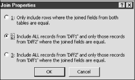
Now switch to the Query tab, and start a new query. Add both Diff1 and Diff2 to the query. You may notice a connecting line between the two ISBN attributes. If there is no such line, drag one ISBN name to the other to create a line. Now right click on the line and choose Join Properties from the pop-up menu. This should produce the dialog box shown in Figure 5-5. Select option 2, which will include all records (rows) from Diff1 and all rows of Diff2 that have a matching ISBN in Diff1. This is a so-called left outer join . We will discuss this in more detail later in this section. Click OK.
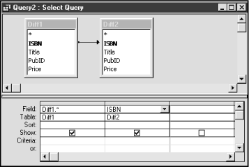
Drag the asterisk (*) from Diff1 to the design grid, and then drag ISBN from Diff2 to the second column of the design grid. The design window should now appear as in Figure 5-6.
Now run the query. You should get a table as shown in Figure 5-7. This table contains the ten rows from Diff1, with an extra column that gives the matching ISBN from Diff2, if there is one. Otherwise, the column contains a NULL. We can see that the six rows that have a matching ISBN in column Diff2.ISBN form the intersection of the two tables. Also, the four rows that do not have a matching ISBN form the difference Diff1 - Diff2. Hence, we only need to add a simple criterion to the query to obtain either the intersection or the difference.
To get the intersection Diff1 ∩ Diff2, return to the design view of the query, and add the words Is Not Null under the Criteria row in the Diff2.ISBN column. Run the query.
To get the difference Diff1 - Diff2, return to the design view of the query, and add the words Is Null under the Criteria row in the Diff2.ISBN column. Run the query.

Cartesian Product
To define the Cartesian product of tables, we need to adjust the way we write attribute names, just in case both tables have an attribute of the same name. If a table T has an attribute named A, the fully qualified attribute name (or just qualified attribute name ) is T.A. Thus, we may write BOOKS.ISBN or AUTHORS.AuID.
If S(A1,...,An) and T(B1,...,Bm) are tables, then the Cartesian product S x T of S and T is the table whose attribute set contains the fully qualified attribute names of all attributes from S and T:
| {S.A1,...,S.An,T.B1,...,T.Bm} |
The rows of S x T are formed by combining each row s of S with each rowtof T, to form a new rowst. An example will help make this clear:
Notice that if S has k rows and T has j rows, then the Cartesian product has kj rows. Hence, the Cartesian product of two tables can be very large.
To form a Cartesian product of two tables in Microsoft Access, proceed as follows:
Create the two tables S and T in the previous example.
Create a new query, and add the tables S and T. Make certain that there are no lines joining the two table schemes. (If there are, right click on the lines, and choose Delete from the pop-up menu.)
Drag the asterisks from each table scheme to the design grid. You should now have a design window as shown in Figure 5-8. Run the query to get the Cartesian product.
Projection
Projection is a very simple concept. Intuitively, a projection of a table onto a subset of its attributes (columns) is the table formed by throwing away all other columns.
More formally, let T(A1,...An) be a table, where A = {A1,...,An} is the attribute set. If B is a subset of A, then the projection of T onto B is just the table obtained from T by keeping only those columns headed by the attribute names in B. We denote this table by proj B (T).
As an example, for the table:
ISBN | Title | Price | PubID |
0-103-45678-9 | The Firm | $24.95 | 1 |
0-11-345678-9 | Moby-Dick | $49.00 | 2 |
0-12-333433-3 | War and Peace | $25.00 | 1 |
the projection proj ISBN,Price(BOOKS) is:
Note that, if the projection produces two identical rows, the duplicate rows must be removed, since a table is not allowed to have duplicate rows. (This rule of relational databases is not enforced by all commercial database products. In particular, it is not enforced by Microsoft Access. That is, some products allow identical rows in a table. By definition, these products are not true relational databases—but that is not necessarily a flaw.)
The Query Design window in Microsoft Access was tailor-made for creating projections. Just add the table to the design window, and drag the desired attribute names to the design grid. Run the query to get the projection. Figure 5-9 shows the Query Design window for computing the projection of Books onto the attributes ISBN and Price.

Selection
Just as the operation of projection selects only a subset of the columns of a table, so the operation of selection selects a subset of the rows of a table. The first step in defining the operation of selection is to define a selection condition or selection criterion to be any legally formed expression that involves:
Constants (i.e., members of any attribute domain)
Attribute names
Arithmetic comparison relations (=, ≠, <, ≤, >, ≥)
Logical operators (and, or, not)
For example, the following are selection conditions:
Price > $10.00
Price ≤ $50.00 and AuName = “Bronte”
(Price ≤ $50.00 and AuName = “Bronte”) or (not AuName = “Austen”)
If condition is a selection condition, then the result table obtained by applying the corresponding selection operation to a table T is denoted by:
sel condition(T)
or sometimes by:
T where condition
and is the table obtained from T by keeping only those rows that satisfy the selection condition.
For example, see Table 5-7.
ISBN | Title | PubID | Price |
0-103-45678-9 | Iliad | 1 | $25.00 |
0-11-345678-9 | Moby-Dick | 3 | $49.00 |
0-12-333433-3 | On Liberty | 1 | $25.00 |
0-12-345678-9 | Jane Eyre | 3 | $49.00 |
0-123-45678-0 | Ulysses | 2 | $34.00 |
0-321-32132-1 | Balloon | 3 | $34.00 |
0-55-123456-9 | Main Street | 3 | $22.95 |
0-555-55555-9 | Macbeth | 2 | $12.00 |
0-91-045678-5 | Hamlet | 2 | $20.00 |
0-91-335678-7 | Faerie Queene | 1 | $15.00 |
0-99-777777-7 | King Lear | 2 | $49.00 |
0-99-999999-9 | Emma | 1 | $20.00 |
1-1111-1111-1 | C++ | 1 | $29.95 |
1-22-233700-0 | Visual Basic | 1 | $25.00 |
The table selPrice $25.00(BOOKS) is shown in Table 5-8:
ISBN | Title | PubID | Price |
0-12-345678-9 | Jane Eyre | 3 | $49.00 |
0-11-345678-9 | Moby-Dick | 3 | $49.00 |
0-99-777777-7 | King Lear | 2 | $49.00 |
0-123-45678-0 | Ulysses | 2 | $34.00 |
1-1111-1111-1 | C++ | 1 | $29.95 |
0-321-32132-1 | Balloon | 3 | $34.00 |
Some authors refer to selection as restriction, which does seem to be a more appropriate term and has the advantage that it is not confused with the SQL SELECT statement, which is much more general than just selection. However, it is less common than the term selection, so we will use this term.
The Query Design window in Microsoft Access was also tailor-made for creating selections. We just use the Criteria rows to apply the desired restrictions. For example, Figure 5-10 shows the design window for the selection:
selPrice $25.00(BOOKS)
from the previous example.

You will probably agree that the operations we have covered so far are pretty straightforward—union, intersection, difference, and Cartesian product are basic set-theoretic operations. Selecting rows and columns are clearly valuable table operations.
Actually, the six operations of renaming, union, difference, Cartesian product, projection, and selection are enough to form the complete relational algebra by combining these operations with constants and attribute names to create relational-algebra expressions.
However, it is very convenient to define some additional operations on tables, even though they can theoretically be expressed in terms of the six operations previously mentioned. So let us proceed.
Joins
The various types of joins are among the most important and useful of the relational-algebra operations. Loosely speaking, joining two tables involves combining the rows of two tables based on comparing the values in selected columns.
Equi-join
In an equi-join, rows are combined if there are equal attribute values in certain selected columns from each table.
To be specific, let S and T be tables, and suppose that {C1,...,Ck} are selected attributes of S and {D1,...,Dk} are selected attributes of T. Each table may have additional attributes as well. Note that we select the same number of attributes from each table.
The equi-join of S and T on columns {C1,...,Ck} and {D1,...,Dk} is the table formed by combining a row of S with a row of T, provided that corresponding columns have equal value—that is, provided that:
S.C 1 = T.D 1,S.C 2, ...,S.C k = T.Dk
As an example, consider the tables:
To form the equi-join:
S equi-joinA2 = B3 T
we combine rows for which:
S.A 2 = T.B 3
This gives:
Notice that the equi-join can be expressed in terms of the Cartesian product and the selection operation as follows:
This simply says that, to form the equi-join, we take the Cartesian product S x T of S and T (i.e., the set of all combinations of rows from S and T) and then select only those rows for which:
S.C 1 T.D 1,S.C 2 = T.D 2, ...,S.Ck = T.D2 , ...,S.Ck = T.Dk
Natural join
The natural join (nat-join) is a variation on the equi-join, based on the equality of allcommon attributes in two tables.
To be specific, suppose that S and T are tables and that the set of all common attributes between these tables is {C1,...,Cn}. Thus, each table may have additional attributes, but no further attributes in common. The natural join of S and T, which we denote by:
S nat-join T
is formed in two steps:
Form the equi-join on the common attributes {C1,...,Cn}.
Remove the second set of common columns from the table.
Consider these tables:
In this case, the set of common attributes is {A2,A4}. The corresponding columns are shaded for easier identification.
The equi-join on A2 and A4 is:
Deleting the second set of common columns (the columns that come from T, as shaded in the previous table) gives:
The importance of the natural join comes from the fact that, when there is a one-to-many relationship from S to T, we can arrange it—by renaming, if necessary—so that the only common attributes are the key of S and the foreign key in T. In this case, the natural join S nat-join T is simply the table obtained by matching rows that are related through the one-to-many relationship.
For example, consider the following BOOKS and PUBLISHERS tables in Tables Table 5-9 and Table 5-10, respectively.
ISBN | Title | Price | PubID |
0-103-45678-9 | The Firm | $24.95 | 1 |
0-11-345678-9 | Moby-Dick | $49.00 | 2 |
0-12-333433-3 | War and Peace | $25.00 | 1 |
0-12-345678-9 | Jane Eyre | $34.00 | 1 |
0-26-888888-8 | Persuasion | $13.00 | 3 |
0-555-55555-9 | Emma | $12.00 | 3 |
0-91-045678-5 | The Chamber | $20.00 | 3 |
0-91-335678-7 | Partners | $15.00 | 1 |
0-99-777777-7 | Triple Play | $44.00 | 3 |
0-99-999999-9 | Mansfield Park | $18.00 | 1 |
PubID | PubName | PubPhone |
1 | Big House | 212-000-1212 |
2 | Little House | 213-111-1212 |
3 | Medium House | 614-222-1212 |
Then PUBLISHERS nat-join BOOKS is the table formed by taking each PUBLISHERS row and adjoining each BOOKS row with a matching PubID, as shown in Table 5-11.
PubID | PubName | PubPhone | ISBN | Title | Price |
1 | Big House | 212-000-1212 | 0-103-45678-9 | The Firm | $24.95 |
1 | Big House | 212-000-1212 | 0-12-333433-3 | War and Peace | $25.00 |
1 | Big House | 212-000-1212 | 0-12-345678-9 | Jane Eyre | $34.00 |
1 | Big House | 212-000-1212 | 0-91-335678-7 | Partners | $15.00 |
1 | Big House | 212-000-1212 | 0-99-999999-9 | Mansfield Park | $18.00 |
2 | Little House | 213-111-1212 | 0-11-345678-9 | Moby-Dick | $49.00 |
3 | Medium House | 614-222-1212 | 0-26-888888-8 | Persuasion | $13.00 |
3 | Medium House | 614-222-1212 | 0-555-55555-9 | Emma | $12.00 |
3 | Medium House | 614-222-1212 | 0-91-045678-5 | The Chamber | $20.00 |
Medium House | 614-222-1212 | 0-99-777777-7 | Triple Play | $44.00 |
θ-Join
The θ-join (read theta join, since θ is the Greek letter theta) is similar to the equi-join and is used when we need to make a comparison other than equality between column values. In fact, the θ-join can use any of these arithmetic comparison relations:
=, ≠, <, ≤, >, ≥
Let S and T be tables, and suppose that {C1,...,Ck} are selected attributes of S and {D1,...,Dk} are selected attributes of T. Each table may have additional attributes as well. Note that we select the same number of attributes from each table. Let θ 1,...,θ k be comparison relations. Then the θ-join of tables S and T on columns C1,...,Ck and D1,...,Dk is:
Thus, to form the θ-join, we take the Cartesian product S x T of S and T and then select those rows for which the value in column C1 stands in relation θ 1 to the value in column D1 and similarly for each of the other columns.
As an example, consider these tables:
To form the θ-join:
we keep only those rows of the Cartesian product of the two tables for which the value in column A2 is ≤ the value in column B3:
Notice that a θ-join, where all relations θ i are equality (=), is precisely the equi-join.
Outer Joins
The natural join, equi-join, and θ-join are referred to as inner joins. Each inner join has a corresponding left outer join and right outer join , which are formed by first taking the corresponding inner join and then including some additional rows.
In particular, for the left outer join, if s is a row of S that was not used in the inner join, we include the row s, filled out to the proper size with NULL values. An example may help to clarify this concept.
In an earlier example, we saw that the natural join of the tables:
is:
The corresponding left outer join is the same as the nat-join, but with a few extra rows:
In particular, the left outer join also contains the two rows of S that were not involved in the natural join, with NULL values used to fill out the rows. The right outer join is defined similarly, where the rows of T are included, with NULL values in place of the S values.
One of the simplest uses for an outer join is to help see what is not part of an inner join! For instance, the previous table shows us instantly that the second and fourth rows:
of table S are not involved in the natural join S nat-join T. Put another way, the values:
and:
Implementing Joins in Microsoft Access
Now let us consider how to implement the various types of joins in Microsoft Access. The Access Query Design window makes it easy to create equi-joins. Of course, a natural join is easily created from an appropriate equi-join by using a projection. Let us illustrate this statement with an example.
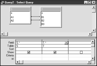
Begin by creating the following two simple tables, S and T, shown in Table 5-12 and Table 5-13.
Let us create the equi-join:
Open the Query Design window (by asking for a new query), and add these two tables. To establish the associations:
S.A 1 = T.B 1
and
S.A 2 = T.B 2
drag the attribute name A1 to B1, and drag the attribute name A2 to B2. This should create the lines shown in Figure 5-11. Drag the two asterisks down to the first two columns of the design grid, as in Figure 5-11. (Access provides the asterisk as a quick way to drag all of the fields to the design grid. It is the same as dragging each field separately with one exception—changes to the underlying table design are reflected in the asterisk. In other words, if new fields are added to the underlying table, they will be included automatically in the query.)
Now all we need to do is run the query. The result is shown in Table 5-14.
In other words, Microsoft Access uses the relationships defined graphically in the upper portion of the window to create an equi-join.
The Access Query Design window does not allow us to create a θ-join that does not use equality. However, we can easily create such a join from an equi-join by altering the corresponding SQL statement. We will discuss SQL in detail in Chapter 6. For now, let us modify the previous example to illustrate the technique.
From the design view for the query in the previous example, select SQL from the View menu. You should see the window shown in Figure 5-12.
This is the SQL statement that Access created from our query design for the previous example. Now, edit the two equal signs by changing each of them to <= (less than or equal to). Note that, for text, the less-than-or-equal-to sign refers to alphabetical order.
Now run the query. The result table should appear as shown in Table 5-15.
A1 | A2 | B1 | B2 | B3 |
a | b | g | h | i |
a | b | j | k | l |
a | b | c | d | x |
a | b | c | d | y |
a | b | c | y | z |
c | d | g | h | i |
c | d | j | k | l |
c | d | c | d | x |
c | d | c | d | y |
c | d | c | y | z |
e | f | g | h | i |
e | f | j | k | l |
Notice that for each row of the table, A1 precedes or equals B1 in alphabetical order, and A2 precedes or equals B2.
Finally, observe that if we try to return to the design view of this query, Access issues the message in Figure 5-13, because the design view cannot create θ-joins that are not based strictly on equality.

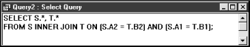
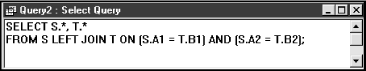
To create an outer join, return the SQL statement of the previous example back to its original form (with equal signs), and then return to design view. Click the right mouse button on one of the connecting lines between the table schemes, and choose Join Properties from the pop-up menu. This should produce the dialog box shown in Figure 5-14.

Select option 2, which will produce a left outer join. (Option 1 creates an inner join, option 2 creates a left outer join, and option 3 creates a right outer join.) Do the same for the other connecting line. Take a peek at the SQL statement, which should appear as in Figure 5-15.
Now you can run the query, which should produce the result table in Table 5-16, where the empty cells contain the NULL value.
Of course, a right outer join is created similarly, by choosing option 3 in Figure 5-14.
Semi-Joins
A semi-join is formed from an inner join (or θ-join) by projecting onto one of the tables that participated in the join. In other words, we first form the join:
and then just keep the columns that came from S or from T. Thus, the formula for the left semi-join is:
Similarly, the formula for the right semi-join is:
The concept of a semi-join occurs in relation to the DISTINCTROW keyword of the SELECT clause in Access SQL, which we will discuss in Chapter 6. For now, let us consider an example of the semi-join, which should indicate why semi-joins are useful.
Imagine that we add a new publisher to the PUBLISHERS table (Another Press in Table 5-17), but do not add any books for this publisher to the BOOKS table. Consider the inner join of the tables PUBLISHERS and BOOKS:
PUBLISHERS join PUBLISHERS.PubID = BOOKS.PubID BOOKS
PubID | PubName | PubPhone |
1 | Big House | 123-456-7890 |
2 | Alpha Press | 999-999-9999 |
3 | Small House | 714-000-0000 |
4 | Another Press | 111-222-3333 |
For the LIBRARY database, the result table resulting from this join is shown in Table 5-18.
PUBLISHERS.PubID | Pub-Name | PubPhone | ISBN | Title | BOOKS.PubID | Price |
3 | Small House | 714-000-0000 | 0-12-345678-9 | Jane Eyre | 3 | $49.00 |
3 | Small House | 714-000-0000 | 0-11-345678-9 | Moby-Dick | 3 | $49.00 |
3 | Small House | 714-000-0000 | 0-321-32132-1 | Balloon | 3 | $34.00 |
3 | Small House | 714-000-0000 | 0-55-123456-9 | Main Street | 3 | $22.95 |
1 | Big House | 123-456-7890 | 0-12-333433-3 | On Liberty | 1 | $25.00 |
1 | Big House | 123-456-7890 | 0-103-45678-9 | Iliad | 1 | $25.00 |
1 | Big House | 123-456-7890 | 0-91-335678-7 | Faerie Queene | 1 | $15.00 |
1 | Big House | 123-456-7890 | 0-99-999999-9 | Emma | 1 | $20.00 |
1 | Big House | 123-456-7890 | 1-22-233700-0 | Visual Basic | 1 | $25.00 |
1 | Big House | 123-456-7890 | 1-1111-1111-1 | C++ | 1 | $29.95 |
2 | Alpha Press | 999-999-9999 | 0-91-045678-5 | Hamlet | 2 | $20.00 |
2 | Alpha Press | 999-999-9999 | 0-555-55555-9 | Macbeth | 2 | $12.00 |
2 | Alpha Press | 999-999-9999 | 0-99-777777-7 | King Lear | 2 | $49.00 |
2 | Alpha Press | 999-999-9999 | 0-123-45678-0 | Ulysses | 2 | $34.00 |
If we now project onto the PUBLISHERS table, we get the left semi-join:
PUBLISHERS left-semi-join PUBLISHERS.PubID = BOOKS.PubID BOOKS
for which the result table is shown in Table 5-19.
PubID | PubName | PubPhone |
3 | Small House | 714-000-0000 |
1 | Big House | 123-456-7890 |
2 | Alpha Press | 999-999-9999 |
This is the set of all publishers that have book entries in the BOOKS database.
Other Relational Algebra Operations
There is one more operation in relational algebra that occurs from time to time, called the quotient . However, since this operation is less common, and a bit involved, we will cover it in Appendix B. (You may turn to that appendix after finishing this chapter, if you are interested.)
Optimization
Let us conclude this discussion with a brief remark about optimization . As we have discussed, statements in the relational algebra are procedural; that is, they describe a procedure for carrying out the operations. However, this procedure is often not very efficient.
Let us illustrate with an extreme example. Consider the two table schemes:
{ISBN,Title,Price} and {ISBN,PageCount}
If S is a table based on the first scheme and T is a table based on the second scheme, then the natural join is:
According to this formula, the join is carried out in the following steps:
Form the Cartesian product.
Take the appropriate selection.
Take the appropriate projection.
Now imagine two tables S and T, where S has 10,000 rows and T has 10,000 rows. Assume also that the tables have only one common attribute, for which no values are the same in both tables. In this case, according to the definition of natural join, the join is actually the empty table.
However, according to the procedure described, the first step in computing this join is to compute the product S x T, which has 10,000 x 10,000 = 100,000,000 rows—that is, one hundred million rows! Obviously, this is not the best procedure for computing the join!
Fortunately, database programs that use a procedural language have optimization routines to avoid problems such as this. Such a routine looks at the task it is requested to perform and tries to find an alternative procedure that will produce the same output with less computation. Thus, from a practical standpoint, procedural languages sometimes behave similarly to nonprocedural ones.