A column definition is defined as follows:

ColumnDefinition ::=ColumnName 
                      DataType[(Size)]
                          [Single-ColumnConstraint]

In words, a ColumnDefinition is a ColumnName, followed by a DataType (with size if appropriate), followed by a Single-ColumnConstraint.

There are several data types available in Access SQL. For comparison, the list in Table 6-2 includes the corresponding selection in the Access Table Design window. (We have not included all synonyms for the data types.) Note that the SQL type INTEGER corresponds with the Access data type Long. Note also that the Size option affects only TEXT columns, indicating the length of the field. (If it is omitted, the text length defaults to 255.)

Constraint clauses can be used to:

(In SQL-92, these clauses have two other uses: to disallow NULLs and to restrict allowable values to a specified range.)

There are two types of constraint clauses in a CREATE TABLE command. The single-column constraint is used (as indicated in the syntax) within a column definition. Its syntax is:

Single-ColumnConstraint ::=
CONSTRAINTIndexName 
 [PRIMARY KEY |
 UNIQUE |
    REFERENCES ReferencedTable [(ReferencedColumn,...)] ]

The first option designates the column as a primary key and creates an index file of the name IndexName on that column. The second option designates the column as a (candidate) key and creates a unique index file on that key, by the name IndexName. The third option designates the column as a foreign key that references the ReferencedColumn ,... column(s) of the ReferencedTable. The ReferencedColumn ,... clause is optional if the referenced table has a primary key, since that key will be the referenced key.

For multicolumn constraints, the CONSTRAINT clause must appear after all column definitions and has the syntax:

Multi-ColumnConstraint ::=
CONSTRAINTIndexName 
 [PRIMARY KEY (ColumnName,...) |
 UNIQUE (ColumnName,...) |
 FOREIGN KEY (ReferencingColumn,...) 
    REFERENCES ReferencedTable [(ReferencedColumn,...)] ]

Here are some examples.

Create the Publishers table scheme:

CREATE TABLE PUBLISHERS
(PubID TEXT(10) CONSTRAINT PrimaryKeyName PRIMARY KEY,
PubName TEXT(100),
PubPhone TEXT(20));

Create the Books table scheme, and link to Publishers using PubID as foreign key:

CREATE TABLE BOOKS
(ISBN TEXT(13) CONSTRAINT PrimaryKeyName PRIMARY KEY,
TITLE TEXT(100),
PRICE MONEY,
PubID TEXT(10) CONSTRAINT Test FOREIGN KEY (PubID) REFERENCES
    Publishers 
(PubID) );

The CREATE INDEX command is specific to Access SQL and is not part of the SQL-92 standard.

A table must be closed before it can be deleted or an index can be removed from it.

The INNER JOIN clause in Access SQL actually denotes a θ-join on one or more columns. (See the discussion of joins in Chapter 5.) In particular, the syntax is:

Table1 INNER JOIN Table2 ON Table1.Column1 θ 1 Table2.Column1 [{AND|OR ON Table1.Column2 θ 2 Table2.Column2},...]

where each θ is one of =, <, >, <=, >=, <> (not equal to).

The syntax for an outer join clause is:

Table1 {LEFT [OUTER]} | {RIGHT [OUTER]} JOIN Table2 ON Table1.Column1 θ 1 Table2.Column1 [{AND|OR ON Table1.Column2 θ 2 Table2.Column2},...]

where θ is one of =, <, >, <=, >=, or < >. Note that the word OUTER is optional.

JOIN statements can be nested. Here is an example that joins the BOOKS, AUTHORS, PUBLISHERS, and BOOK/AUTHOR tables and then selects the Title, AuName, and PubName columns. I have indented some lines in the hope of increasing readability. (I will describe the SELECT statement soon.)

SELECT Title, AuName, PubName
FROM 
AUTHORS INNER JOIN 
 (PUBLISHERS INNER JOIN
 (BOOKS INNER JOIN [BOOK/AUTHOR] 
 ON BOOKS.ISBN=[BOOK/AUTHOR].ISBN)
 ON PUBLISHERS.PubID = BOOKS.PubID)
ON AUTHORS.AuID = [BOOK/AUTHOR].AuID;

To see how this was constructed, it helps to look at the relationships between the tables involved. Figure 6-3 shows a portion of the relationships window in Access.

Figure 6-3. A portion of the Relationships window in Access

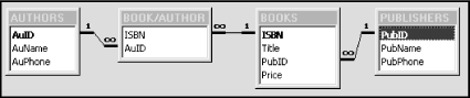
One way to create the previous join statement is to work from the inside out. We first join BOOKS and BOOK/AUTHOR by the statement:

(BOOKS INNER JOIN [BOOK/AUTHOR] 
     ON BOOKS.ISBN=[BOOK/AUTHOR].ISBN)

We then join this to PUBLISHERS on the PubID column:

(PUBLISHERS INNER JOIN
 (BOOKS INNER JOIN [BOOK/AUTHOR] 
 ON BOOKS.ISBN=[BOOK/AUTHOR].ISBN)
ON PUBLISHERS.PubID = BOOKS.PubID)

and finally we join this to AUTHORS on the AuID column.

A table can be joined to itself, resulting in a self-join. In order to do this, SQL requires the use of the AS AliasName syntax. For instance, we can write:

BOOKS INNER JOIN BOOKS AS BOOKS2 ON ...

The least confusing way to think of this statement is as though Access creates a second copy of the BOOKS table and calls it BOOKS2. We can now refer to the columns of BOOKS as BOOKS.ColumnName or BOOKS2.ColumnName.

The predicate is used to describe how to handle duplicate return rows. It can have one of the following values: ALL, DISTINCT, DISTINCTROW, or TOP.

The default option ALL returns all qualifying rows, including duplicates. If there is more than one qualifying row with the same values in all of the columns that arerequested in the ReturnColumnDescription, then the option DISTINCT returns only the first such row. The:

TOPnumber

or:

TOPpercent PERCENT

option returns the top number (or percent) of rows in the sort order determined by the ORDER BY clause.

The DISTINCTROW option can be a bit confusing, so let us see if we can straighten it out. The Access Help system says that the DISTINCTROW option “Omits data based on entire duplicate records, not just duplicate fields.” It doesn’t say how this is done. Microsoft Technet is a bit less vague:

The intended purpose of DISTINCTROW is simple. DISTINCTROW applies only when the FROM clause involves more than one table. Consider this statement:

SELECT ALL PubName
FROM PUBLISHERS INNER JOIN BOOKS
ON PUBLISHERS.PubID = BOOKS.PubID;

Since there are many books published by the same publisher, the result table tblALL shown in Table 6-3 has many duplicate publisher names.

To remove duplicate publisher names, we can include the DISTINCT keyword. Thus, the statement

SELECT DISTINCT PubName
FROM PUBLISHERS INNER JOIN BOOKS
ON PUBLISHERS.PubID = BOOKS.PubID;

produces the table tblDISTINCT that is shown in Table 6-4.

Now consider what happens if the PUBLISHERS table is changed by adding a new publisher with the same name as an existing publisher (but a different PubID and phone), as we have done in Table 6-5. The previous DISTINCT statement will give the same result table as before, thus leaving out the new publisher.

What is called for is a selection criterion that will return both publisher names simply because they come from different rows of the PUBLISHERS table. This is the purpose of DISTINCTROW. Thus, the statement:

SELECT DISTINCTROW PubName
FROM PUBLISHERS INNER JOIN BOOKS
ON PUBLISHERS.PubID = BOOKS.PubID;

produces the result table tblDISTINCTROW shown in Table 6-6 (note that we also had to add a book to the BOOKS table, with PubID 4).

We can now describe how DISTINCTROW works. Consider the following SQL skeleton:

SELECT DISTINCTROWColumnsRequested
FROM TablesClause

Here ColumnsRequested is a list of columns requested by the statement, and TablesClause is a join of tables. Let us refer to a table mentioned in TablesClause as a return table if at least one of its columns is mentioned in ColumnsRequested . Thus, in the statement:

SELECT DISTINCTROW PubName
FROM PUBLISHERS INNER JOIN BOOKS
ON PUBLISHERS.PubID = BOOKS.PubID;

PUBLISHERS is a return table, but BOOKS is not. Here is how DISTINCTROW works:

Let us illustrate with a simple example.

Consider the following tables, named Temp1, Temp2, and Temp3, respectively:

The statement:

SELECT *
FROM 
(Temp1 INNER JOIN Temp2 ON Temp1.A2 = Temp2.B2) 
INNER JOIN Temp3 ON Temp2.B3 = Temp3.C3;

gives the result table tblALL:

Now let us add the DISTINCTROW keyword and select a single column from just tblA:

SELECT DISTINCTROW A1
FROM 
(Temp1 INNER JOIN Temp2 ON Temp1.A2 = Temp2.B2) 
INNER JOIN Temp3 ON Temp2.B3 = Temp3.C3;

Now we consider the projection onto the rows of the only return table (tblA):

It is clear that the first two rows of this table are the same row of tblA, so they produce only one row in the final result table. The same holds for the last two rows. Hence, the result table is:

Let us now change this by requesting a column from tblC, thus making it a return table as well:

SELECT DISTINCTROW A1,C1
FROM 
(Temp1 INNER JOIN Temp2 ON Temp1.A2 = Temp2.B2) 
INNER JOIN Temp3 ON Temp2.B3 = Temp3.C3;

The projection onto return table rows is now:

These row “pairs” are all distinct. In fact:

It follows that the return table includes all rows:

Finally, consider what happens if we change the third row of tblA to:

Running the first DISTINCTROW statement:

SELECT DISTINCTROW A1
FROM 
(Temp1 INNER JOIN Temp2 ON Temp1.A2 = Temp2.B2) 
INNER JOIN Temp3 ON Temp2.B3 = Temp3.C3;

gives:

Comparing this to the previous result table DISTINCTROW, A1 emphasizes the fact that, even though the second and third rows of tblNewA are identical in values, they are different rows, so they both contribute to the final result table. If we were to replace the DISTINCTROW keyword with the word DISTINCT, then the result table would have only one row, since then it is the values in each row that form the basis for comparison.

Of course, this would not be an issue if all tables had a key, since then the values in a row would determine the row. You may now see why I recommended against having two different rows with the same column values, even though Access permits this possibility (but true relational databases do not).

Notice what happens if all tables mentioned in the TablesClause are return tables. This would happen, for instance, if there is only one table in TablesClause. In this case, the projection does nothing; since each row of the TablesClause result table must come from a distinct combination of rows of the result tables, we deduce that DISTINCTROW has exactly the same effect as ALL. To put it another way, DISTINCTROW is ignored.

It is useful to compare DISTINCTROW and DISTINCT. We can see that the only difference is that a DISTINCT statement will return distinct values, rather than values from distinct rows. However, these will be the same if the requested columns from each return table uniquely identify their rows.

Let us illustrate with the PUBLISHERS example. Suppose we return a key (PubID) for PUBLISHERS, as in the statement:

SELECT DISTINCTROW PubID, PubName
FROM PUBLISHERS INNER JOIN BOOKS
ON PUBLISHERS.PubID = BOOKS.PubID;

Then the result table will return all PUBLISHERS rows that have at least one book in the BOOKS table, as Table 6-7 shows.

This is, in fact, the semi-join:

PUBLISHERSsemi-join
                     PUBLISHERS.PubID=BOOKS.PubID
                     BOOKS

Recall that the semi-join is the projection of the join onto one of the tables (in this case, the PUBLISHERS table). Thus, as Microsoft itself says, the purpose of the DISTINCTROW option is to return an updatable semi-join.

Of course, the same statement with DISTINCT in place of DISTINCTROW will return the same result table. However, there is one big difference. Since DISTINCT statements can completely hide the origin of the returned values, it would be a disaster if Access allowed such a result table to be updatable—and indeed it does not. For instance, recall the table tblDISTINCT discussed earlier and shown in Table 6-8.

Changing the name of Small House in this result table would be disastrous, since we would not know which Small House was being affected!

On the other hand, the result table of the DISTINCTROW statement has a “representative” from each row of the PUBLISHERS table, as Table 6-9 shows. Hence, while it still may not be a good idea to change this particular table, since we cannot tell which Small House is which, it would be reasonable to make a change to both names, for instance.

More generally, Access does not permit updating of the result table of a DISTINCT statement, but it does permit updating of the result table for a DISTINCTROW statement.

Finally, we mention that Microsoft Access includes the DISTINCTROW keyword by default when you create a query using the Access Query Design Window.

The ReturnColumnDescription describes the columns, or combination of columns, to return. It can be any of the following:

(Note that, according to the syntax of the SELECT statement, ReturnColumnDescription can be repeated as many times as desired.)

When two returned columns (from different tables) have the same name, it is necessary to qualify the column names using the table names. For instance, to qualify the PubID column name, we write BOOKS.PubID and PUBLISHERS.PubID. We can also write BOOKS.* to indicate all columns of the BOOKS table.

Finally, each ReturnColumnDescription can end with:

[AS AliasName]

to give the return column a (new) name. For example, the following statement:

SELECT DISTINCTROW 
[ISBN] & " from " & [PubName] AS [ISBN from PubName] 
FROM PUBLISHERS INNER JOIN BOOKS ON PUBLISHERS.PubID = BOOKS.PubID;

returns a single-column result table ISBN-PUB, as shown in Table 6-10.

Not only does the AS AliasName option allow us to name a compound column, it also allows us to rename duplicate column names without having to qualify the names.

The FROM clause specifies the tables (or queries) from which the SELECT statement is to take its rows. The expression TableExpression can be a single table name, several table names separated by commas, or a join clause. The TableExpression may also include the AS AliasName syntax for table-name aliases.

When tables are separated by commas in the FROM clause, a Cartesian product is formed. For example, the statement:

SELECT *
FROM AUTHORS, PUBLISHERS;

will produce the Cartesian product of the two tables.

The RowCondition is any Access expression that specifies which rows are included in the result table. Expressions can involve column names, constants, arithmetic (=, <, >, <=, >=, < >, BETWEEN) and logical (AND, OR, XOR, NOT, IMP) relations, as well as functions. Here are some examples:

Note that dates are enclosed in number signs (#) and the strings are enclosed in quotation marks (” “).

The GROUP BY option allows records to be grouped together for the purpose of computing the value of an aggregate function (Avg, Count, Min, Max, Sum, First, Last, StDev, StDevP, Var, and VarP). It is equivalent to creating a so-called totals query. The GroupByCriteria can contain the names of up to 10 columns. The order of the column names determines the grouping levels, from highest to lowest.

For example, the following statement lists each publisher by name, along with the minimum price of each publisher’s books in the BOOKS table:

SELECT PUBLISHERS.PubName, MIN(Price) AS [Minimum Price]
FROM PUBLISHERS INNER JOIN BOOKS
ON PUBLISHERS.PubID = BOOKS.PubID
GROUP BY PUBLISHERS.PubName;

The result table appears in Table 6-11.

The HAVING option is used in conjunction with the GROUP BY option and allows us to specify a criterion, in terms of aggregate functions, for deciding which data to display.

For example, the following command is the same as the previous one, with the additional HAVING option that restricts the return table to those publishers whose minimum price is less than $20.00:

SELECT PUBLISHERS.PubName, MIN(Price) AS [Minimum Price]
FROM PUBLISHERS INNER JOIN BOOKS
ON PUBLISHERS.PubID = BOOKS.PubID
GROUP BY PUBLISHERS.PubName
HAVING MIN(Price)<20.00;

The result table is shown in Table 6-12.

Note that the WHERE clause restricts which rows participate in the grouping and hence contribute to the value of the aggregate functions, whereas the HAVING clause affects only which values are displayed.

The ORDER BY option describes the order in which to return the rows in the return table. The OrderByCriteria has the form:

OrderByCriteria ::= {ColumnName [ASC | DESC ]},...

In other words, it is just a list of columns to use in the ordering. Rows are sorted first by the first column listed, then rows with identical values in the first column are sorted by the values in the second column, and so on.

The following statement takes the union of all rows of BOOKS and those rows of NEWBOOKS that have Price > $25.00, sorting the result table by Title:

TABLE BOOKS
UNION ALL
SELECT * FROM NEWBOOKS WHERE Price > 25.00
ORDER BY Title;

The following example updates the Price column in the BOOKS table with new prices from a table called NEWPRICES that has an ISBN and a Price column:

UPDATE 
BOOKS INNER JOIN NEWPRICES ON BOOKS.ISBN = NEWPRICES.ISBN
SET BOOKS.Price = NEWPRICES.Price
WHERE BOOKS.Price <> NEWPRICES.Price;

Note that UPDATE does not produce a result table. To determine which rows will be updated, first run a corresponding SELECT query, as in:

SELECT * FROM 
BOOKS INNER JOIN NEWPRICES ON BOOKS.ISBN = NEWPRICES.ISBN
WHERE BOOKS.Price <> NEWPRICES.Price

Text field values must be enclosed in quotation marks.

Comparison [ANY | SOME | ALL] (SQLStatement)

where Comparison is an expression followed by a comparison relation that compares the expression with the return value(s) of the subquery. This syntax is used to compare a value against the values obtained from another query.

For example, the following statement returns all titles and prices of books from the BOOKS table, whose prices are greater than the maximum price of all books in the table BOOKS2:

SELECT Title, Price
FROM BOOKS
WHERE Price > (SELECT Max(Price) FROM BOOKS2);

Note that since the subquery returns only one value, we do not need to use any of the keywords ANY, SOME, or ALL.

The following statement selects all BOOKS titles and prices for books that are more expensive than ALL of the books published by Big House:

SELECT Title, Price
FROM BOOKS
WHERE Price > ALL
   (SELECT Price 
   FROM PUBLISHERS INNER JOIN BOOKS ON PUBLISHERS.PubID = 
   BOOKS.PubID
   WHERE PubName = "Big House");

Note that ANY and SOME have the same meaning and return all choices that make the comparison true for at least one value returned by the subquery. For example, if we were to replace ALL by SOME in the previous example, the return table would consist of all book titles and prices for books that are more expensive than the cheapest book published by Big House.

Expression [NOT] IN (SQLStatement)

This syntax is used to look up a column value in the result table of another query.

For example, the following statement returns all book titles from BOOKS that do not appear in the table BOOKS2:

SELECT Title
FROM BOOKS
WHERE Title NOT IN (SELECT Title FROM BOOKS2);

[NOT] EXISTS (SQLStatement)

This syntax is used to check whether an item exists (is returned) in the subquery.

For example, the following statement selects all publishers that do not have books in the BOOKS table:

SELECT PubName
FROM PUBLISHERS
WHERE NOT EXISTS 
 (SELECT * FROM BOOKS WHERE BOOKS.PubID =
 PUBLISHERS.PubID);

Notice that the PUBLISHERS table is referenced in the subquery. This causes Access to evaluate the subquery once for each value of PUBLISHERS.PubID in the PUBLISHERS table.