Chapter 4
An Introduction to Derivative Instruments
Before addressing the hedge accounting implications of the most common hedging strategies, it is helpful to examine the most common derivative instruments used in these strategies. The main characteristics of each derivative are described and, where relevant, its accounting implications under IFRS 9 are highlighted. A more detailed explanation of the accounting issues related to a specific derivative may be found in the numerous cases provided in this book.
4.1 FX FORWARDS
4.1.1 Product Description
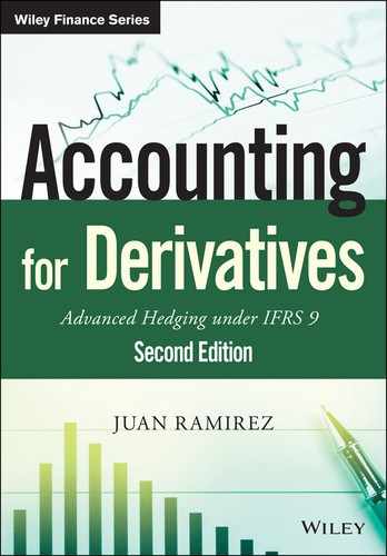
An FX forward is the most common and simplest hedging instrument in the FX market. It is a contract to exchange a fixed amount of one currency for a fixed amount of another currency on a specific future date. Suppose that on 1 January 20X5 ABC, a European company, expects to purchase a USD 100 million machine from a US supplier. The purchase is expected to be paid in USD on 30 June 20X5. As a result, ABC is exposed, from the moment it places the order until it makes the payment, to an appreciation of the USD relative to the EUR. To hedge this exposure ABC may enter into an FX forward with the following terms:
| FX forward terms | |
| Trade date | 1 January 20X5 |
| Counterparties | ABC and XYZ Bank |
| Maturity | 30 June 20X5 |
| ABC buys | USD 100 million |
| ABC sells | EUR 80 million |
| Forward Rate | 1.2500 |
| Settlement | Physical delivery |
The FX forward locks in the exchange rate at which ABC will buy USD 100 million. In other words, ABC knows that (unless XYZ Bank defaults) on 30 June 20X5 it will receive USD 100 million in exchange for EUR 80 million (i.e., at an exchange rate of 1.2500), whatever the level of the EUR–USD exchange rate (i.e., the number of USD in exchange for 1 EUR) on that date (see Figures 4.1 and 4.2). ABC will use the received USD 100 million to pay the US supplier. The 1.2500 forward rate is, as of 1 January 20X5, the market expected EUR–USD rate for 30 June 20X5, so no premium is paid by either of the two parties to the forward at the beginning of the transaction.
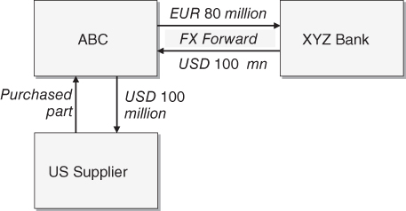
Figure 4.1 FX forward cash flows.
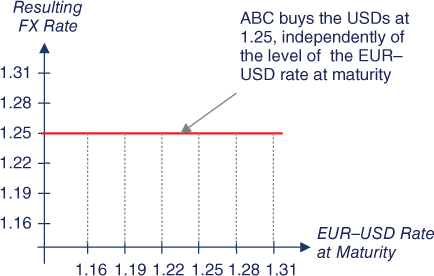
Figure 4.2 FX forward – resulting FX rate.
Similarly, the hedge can be analysed by looking at the amount of EUR that ABC will need to sell in order to buy the USD 100 million at maturity, as a function of the EUR–USD exchange rate. Figure 4.3 shows that the FX forward locks in a EUR 80 million amount, whatever the EUR–USD rate at maturity.

Figure 4.3 FX forward – EUR amount.
Forward contracts may be settled by physical delivery or by cash settlement. The FX forward described previously will be settled by physical delivery. As a consequence, the parties will actually exchange currencies on 30 June 20X5: ABC agrees to buy USD 100 million and, simultaneously, to sell EUR 80 million. If the contract were to be settled by cash settlement, a final exchange rate would be set by observing an official fixing two business days prior to the maturity date, and then one counterparty will pay the other a settlement amount. For example, if two business days prior to maturity the official EUR–USD rate fixes at 1.3000, ABC would pay to XYZ Bank on 30 June 20X5 EUR 3,076,923.08 (=100 million × (1/1.2500 – 1/1.3000)).
4.1.2 Forward Points
An FX forward is arguably the friendliest FX hedging instrument from the perspective of IFRS 9. The only particular point to note is the accounting treatment of the forward points. The forward points are the difference between the forward and spot prices. For example, if on 1 January 20X5 the spot EUR–USD rate was 1.2360 and the EUR–USD forward rate for 30 June 20X5 was 1.2500, then the forward points were 0.0140 (=1.2500 – 1.2360). The forward points reflect the differential between USD and EUR interest rates from 1 January 20X5 to 30 June 20X5.
At maturity of the transaction the forward points become zero as spot and forward rates converge, as shown in Figure 4.4 (assuming that the EUR–USD spot rate on 30 June 20X5 trades at 1.3020).

Figure 4.4 FX forward and spot rates convergence at maturity.
The accounting treatment for forward contracts when hedge accounting is applied is covered in Chapter 2.
4.2 INTEREST RATE SWAPS
4.2.1 Product Description
An interest rate swap (often simply called a “swap”) is the most commonly used instrument to hedge interest rate risk. In general, a swap is an exchange of interest payment flows in the same currency. Swaps are mostly used to change the interest rate risk profile of interest-bearing assets and/or liabilities.
Corporations and financial institutions usually enter into swaps to transform the interest rate basis of a debt instrument from a floating to fixed rate or vice versa. The two parties to a swap agree to exchange, at certain future dates, two sets of cash flows denominated in the same currency. The cash flows paid by one party reflect a fixed rate of interest while those of the other party reflect a floating rate of interest. The term “floating rate” or “variable rate” means that the interest rate used in an interest period is unknown until the commencement of such period. In the case of Euribor interest rates, the floating rate of a specific interest period is set two business days prior to the beginning of the interest period. All the stream of fixed rate payments is grouped together under the term fixed leg. Similarly, the floating leg groups all the floating rate payments. The swap is usually entered at market rates, and as a result there is no exchange of a premium at the inception of the swap.
The following example highlights the mechanics of swaps. On 15 January 20X0, ABC enters into a EUR 100 million notional, 3-year interest rate swap. Pursuant to the terms of the swap, ABC will pay semiannually a 5% fixed interest and receive annually a floating interest (Euribor 12-month rate), both calculated on the notional amount. The floating interest rate resets two business days prior to the commencement of each interest period (in accordance with the Euribor market convention). The terms of the swap are summarised below:
| Interest rate swap terms | |
| Trade date | 15 January 20X0 |
| Parties | ABC and XYZ Bank |
| Maturity | 3 years (15 January 20X3) |
| Notional | EUR 100 million |
| ABC pays | 5.00% semiannually, 30/360 basis |
| ABC receives | Euribor 12-month annually, actual/360 basis Euribor 12-month is fixed two business days prior to the beginning of the annual interest period |
The fixed leg of this swap has six interest periods, while the floating leg has three. Figure 4.5 shows the cash flow dates of the fixed and floating legs.

Figure 4.5 Interest rate swap flows.
All the future fixed leg cash flows are known at the beginning of the swap. ABC will be paying EUR 2.5 million (=100,000,000 × 5%/2) on 15 July and 15 January every year during the life of the swap, starting on 15 July 20X0.
Unlike the fixed leg cash flows, the future floating leg cash flows are unknown at the beginning of the swap (except the first one). The first floating cash flow will take place on 15 January 20X1 and its floating rate (i.e., 2.70%) is already known at the swap inception as it was fixed on 13 January 20X0 (i.e., two business days prior to the beginning of the first interest period). As a result, ABC expects to receive EUR 2,737,500 (=100,000,000 × 2.70% × 365/360) on 15 January 20X1, assuming 365 calendar days between 15 January 20X0 and 15 January 20X1. Each of the remaining floating leg cash flows will be determined two business days prior to the beginning of their corresponding interest period. For example, the cash flow to be received by ABC on 15 January 20X2 will be known on 13 January 20X1. There are several examples of swaps and their pricing mechanics in the cases covered in Chapter 7.
4.2.2 IFRS 9 Accounting Implications
Interest rate swaps are the friendliest interest rate hedging instruments from the perspective of IFRS 9. There are two particular points that are covered in detail in Chapter 7 that I would like to highlight: firstly, the need to define hedging relationships involving swaps in such a way that eligibility for hedge accounting is maximised; and secondly, the need to exclude interest accrual amounts when calculating swap fair value changes.
In a hedge accounting context, a swap is often linked to a specific debt instrument (asset or liability). The market value of a swap and the debt instrument are usually determined using different yield curves. Typically, the market values a debt instrument using a yield curve that incorporates the issuer's credit spread, while swaps are valued by excluding credit spreads from the yield curve and subsequently credit/debit valuation adjusted to incorporate either the entity or the counterparty credit risk (see Chapter 3 for a more detailed explanation of CVAs and DVAs). As a result the interest rate sensitivities of a debt instrument and its related swap can be significantly different, endangering the eligibility for hedge accounting of a well-constructed hedge. When the debt instrument and the swap interest rate sensitivities are notably different, it is advisable to include in the hedging relationship only the interest rate risk (i.e., excluding other risks, such as the credit risk).
Often valuation dates fall within interest periods. When assessing whether a hedging relationship meets the effectiveness requirements, the inclusion or exclusion of accrued interest in the valuation of a swap may have a substantial impact. The solution to this problem is a simple one: interest accrual amounts need to be excluded when calculating a swap fair value. Excluding interest accrual amounts is especially relevant to making consistent fair value comparisons of debt instruments and swaps with unmatched interest periods. Additionally, excluding interest accrual amounts is also needed to avoid double counting interest income or expenses related to a swap, as the income or expenses associated with a cash flow is apportioned into the periods to which it relates. The calculation of accruals is quite straightforward, as shown in Chapter 7.
4.3 CROSS-CURRENCY SWAPS
4.3.1 Product Description
A cross-currency swap (CCS), or “currency swap” for short, is a contract to exchange interest payment flows in one currency for interest payment flows in another currency. CCSs are mostly used to change the interest rate risk and currency profile of interest-bearing assets and/or liabilities. They are also used to hedge investments in foreign subsidiaries.
Corporations and financial institutions usually enter into CCSs to transform the currency denomination of a debt obligation denominated in a foreign currency. The two parties to a CCS agree to exchange, at certain future dates, two set of cash flows denominated in different currencies. The cash flows paid by one party reflect a fixed (or a floating) rate of interest in one currency while those of the other party reflect a fixed (or floating) rate of interest in another currency.
In its simplest, and most common, form a CCS involves the following cash flows:
- An initial exchange of principal amounts. This initial exchange is sometimes not undertaken. The most common situation in which no initial exchange is needed is when the CCS is being undertaken to hedge already existing liabilities.
- A string of interim interest payments. Periodically, one party pays a fixed (or floating) interest on one of the principal amounts while the other party pays a fixed (or floating) interest on the other principal amounts. The payments are usually netted.
- A final re-exchange of principal amounts.
For example, suppose a borrower (ABC) is about to issue a GBP 70 million 5% fixed rate 5-year GBP-denominated bond. Because the borrower is only interested in raising variable rate EUR funds, it decides to transform the GBP fixed rate liability into a EUR floating rate liability by entering into a CCS. The terms of the bond and the swap are summarised in the following tables:
| Bond terms | |
| Maturity | 5 years |
| Notional | GBP 70 million |
| Coupon | 5%, to be paid annually, 30/360 basis |
| Cross-currency swap terms | |
| Maturity date | 5 years |
| Parties | ABC and Megabank |
| GBP nominal | GBP 70 million |
| EUR nominal | EUR 100 million |
| Initial exchange | On start date, ABC receives the EUR nominal and pays the GBP nominal |
| ABC pays | Euribor 12-month + 50 bps annually, actual/360 basis, on the EUR nominal |
| ABC receives | GBP 5% annually, on the GBP nominal |
| Final exchange | On maturity date, ABC receives the GBP nominal and pays the EUR nominal |
Figure 4.6 shows the initial cash flows of the CCS and their interaction with the bond's initial flow. Through the CCS, the ABC delivers GBP 70 million (i.e., the issue proceeds) and receives EUR 100 million. As a result, ABC is in effect raising EUR funding.

Figure 4.6 Bond and CCS: initial cash flows.
Figure 4.7 depicts the periodic interest payments of the bond and the CCS. Through the CCS, ABC receives from Megabank an annual GBP 5% interest calculated on the GBP 70 million nominal, and pays annually to Megabank a EUR floating interest (Euribor 12-month plus 50 basis points) calculated on the EUR 100 million nominal. The borrower uses the CCS GBP receipts to meet the bond interest payments.
Figure 4.7 Bond and CCS: interim cash flows.
Figure 4.8 shows the CCS final cash flows and their interaction with the bond's redemption. On maturity date ABC re-exchanges the notionals, paying EUR 100 million and receiving GBP 70 million through the CCS. ABC then uses the received GBP 70 million to repay the GBP bond.

Figure 4.8 Bond and CCS: final cash flows.
Under the structure depicted, ABC effectively achieves EUR funding at Euribor plus 50 bps. Note that all the GBP cash flows have to be fully synchronised to eliminate the borrower's GBP exposure. Chapter 8 includes several examples of CCSs and their pricing mechanics.
4.3.2 IFRS 9 Accounting Implications
Cross-currency swaps are the most basic instruments to hedge foreign currency denominated liabilities. From an accounting perspective, as noted above for interest rate swaps, there are two particular points that are worth noting: firstly, there are several sources of ineffectiveness; and secondly, the need to exclude the interest accrual amounts when calculating CCS fair value changes.
In a hedge accounting context, a CCS is often linked to a specific foreign currency denominated liability. The fair value of a CCS contains several elements that may cause hedge ineffectiveness.
Firstly, a CCS fair value is adjusted to incorporate either the CCS counterparty's or the entity's non-performance (i.e., CVA/DVA). In a cash flow hedge, the fair valuation of the hedged cash flows does not incorporate the liability issuer's credit spread. As a result, in a cash flow hedge ineffectiveness may be caused by the CVAs/DVAs to the CCS, which can be substantial when the derivative (i.e., the CCS) is uncollateralised and long-term.
Secondly, a CCS market pricing incorporates a basis (referred to in IFRS 9 as “currency basis spread”), an adjustment to the theoretical CCS pricing that incorporates the appetite of the market for exchanging floating cash flows in the two currencies of the CCS. For example, imagine a floating-to-floating EUR–GBP CCS, in which a Euribor-linked EUR leg is exchanged for a Libor-linked GBP leg. Strong demand for receiving Euribor flows may lead to a Euribor-linked EUR leg being exchanged for a Libor-linked plus a spread GBP leg. This spread is commonly referred to as the basis. During the life of a CCS, the basis may fluctuate, affecting the CCS's fair value. Because the hedged liability (i.e., the hedged item) is not affected by the basis, fluctuations in the CCS basis may cause ineffectiveness. IFRS 9, similarly to the treatment of the forward element in forward contracts, allows the exclusion of the basis from the hedging relationship and temporary recognition of the change in the fair value of the basis element in OCI to the extent that it relates to the hedged item.
Thirdly, in a fair value hedge, the fair valuation of a CCS and its related liability may be determined using different yield curves. Commonly, when a CCS is collateralised (i.e., each party to the CCS posts/receives collateral to eliminate counterparty credit risk exposure) an OIS yield curve is used to fair value the CCS. The fair valuation of the hedged liability is performed using a non-OIS curve (typically a Euribor or Libor based yield curve). As a result the interest rate sensitivities of a liability and its related CCS can be significantly different, causing ineffectiveness even in a well-constructed hedge. When a liability and its CCS rate sensitivities are notably different, it is suggested that the hedging relationship is defined as the hedge of interest rate and FX risk only (i.e., excluding the liability's credit spread).
Often valuation dates fall within interest periods. The inclusion or exclusion of accrued interest in the valuation of a CCS can make a substantial difference. The solution to this problem is to exclude interest accrual amounts when calculating a CCS fair value. The exclusion is especially important in making consistent fair value comparisons of liabilities and CCS with different interest periods. The exclusion is also needed to avoid double counting the interest income or expenses related to a CCS, as the income or expenses associated with a cash flow is apportioned into the periods to which it relates. Chapter 8 includes detailed computations of the interest accruals of CCSs.
In addition to hedging foreign currency denominated liabilities, CCSs are used to hedge the FX exposure of net investments in foreign operations. For that type of hedge, IFRS 9 sets a special type of hedge accounting, called a “net investment hedge”. When designated as hedging instruments of net investment hedges, some aspects of the accounting treatment of CCSs are unclear. This is particularly the case for CCSs in which the entity pays a fixed interest rate in the leg denominated in the group's functional currency leg. This accounting uncertainty is covered in more detail in Chapter 6.
4.4 STANDARD (VANILLA) OPTIONS
In this section the mechanics of standard options are described. Under IFRS 9, the accounting for an option's time value, when excluded from a hedging relationship, follows a particular treatment which was covered in detail in Chapter 2.
4.4.1 Product Description
In general there are two types of options: standard options and exotic options. Standard options, also called “vanilla options” or just “options”, are the most basic option instruments. Unlike the terms of most exotic options, the terms of a standard option (nominal, strike, expiry date, etc.) are known at its inception. There are two types of standard options:
- Call options. A call gives the buyer the right, but not the obligation, to buy a specific amount of an underlying at a predetermined price on or before a specific future date.
- Put options. A put gives the buyer the right, but not the obligation, to sell a specific amount of an underlying at a predetermined price on or before a specific future date.
The buyer of the option has to pay a premium to the seller. Usually the premium is paid shortly after the option is agreed (e.g., two business days after trade date). The underlying can be any financial asset (e.g., a security, a currency, a commodity) or a financial index (e.g., a stock market index, an interest rate).
4.4.2 Standard Equity Options
Equity options are a means for their buyers to gain either long or short exposure to an equity underlying with a limited downside.
Call Options
Equity call options allow an investor to take a bullish view on an underlying stock, a basket of stocks or a stock index.
- A physically settled European call option provides the buyer (the holder) the right, but not the obligation, to buy a specified number of shares of an equity underlying at a predetermined price (the strike price) at a future date (the expiration date). In return for this right, the buyer pays an up-front premium for the call.
- A cash-settled European call option provides the buyer the appreciation (i.e., the increase in value of the underlying shares relative to the strike price) of a specified number of shares of an equity underlying above a predetermined price (the strike price) at a future date (the expiration date). The buyer pays an up-front premium for the call.
At expiry, the holder of the call will exercise the option if the share price of the underlying stock is higher than the strike price. Thus, if the share price ends up lower than the strike price, the holder will not exercise the call. The holder has unlimited upside potential, while his/her loss is limited to the option premium paid.
As an example, suppose that on 3 June 20X1 ABC is looking to buy IBM stock in 6 months' time. ABC believes that IBM stock will significantly increase in value over the next 6 months and acquires from Gigabank a European call option on 1 million IBM shares. On 3 June 20X1, IBM stock is trading at USD 150. The physically settled call option has the following terms:
| Physically settled call option – main terms | |
| Buyer | ABC Corp. |
| Seller | Gigabank |
| Option type | Call |
| Trade date | 3-June-20X1 |
| Expiration date | 3-December-20X1 |
| Option style | European |
| Shares | IBM |
| Number of options | 1 million |
| Option entitlement | One share per option |
| Strike price | USD 180.00 (120% of the spot price) |
| Spot price | USD 150.00 |
| Premium | 2.66% of the notional amount USD 4 million (i.e., USD 4 per share) |
| Premium payment date | Two currency business days after the trade date (5-June-20X1) |
| Notional amount | Number of options × Spot price USD 150 million |
| Settlement method | Physical settlement |
| Settlement date | 6-December-20X1 (three exchange business days after the Expiration date) |
By buying the call option ABC has the right, but not the obligation, to buy on the settlement date 1 million shares of IBM at a strike price of USD 180 per share. Because upon exercise ABC would be buying the underlying stock, the call is a physically settled call. ABC pays Gigabank a premium of USD 4 million on 5 June 20X1. Because it is European-style, the option can only be exercised at expiry. On the expiration date, 3 December 20X1, ABC would be assessing whether to exercise the option, as follows:
- If IBM's stock price is greater than the USD 180 strike price, ABC would exercise the call. On the settlement date ABC would receive from Gigabank 1 million shares of IBM in exchange for USD 180 million. For example, if at expiry IBM stock is trading at USD 210, ABC would exercise the call option paying USD 180 per share for a stock worth USD 210 per share.
- If IBM's stock price is lower than or equal to the USD 180 strike price, ABC would not exercise the option.
In a similar example, suppose that ABC is not interested in having the right to buy 1 million shares of IBM but instead in receiving the appreciation of 1 million shares of IBM above USD 180. ABC then buys a cash-settled European call option on IBM stock with the following terms:
| Cash-settled call option – main terms | |
| Buyer | ABC Corp |
| Seller | Gigabank |
| Option type | Call |
| Trade date | 3-June-20X1 |
| Expiration date | 3-December-20X1 |
| Option style | European |
| Shares | IBM |
| Number of options | 1 million |
| Option entitlement | One share per option |
| Strike price | USD 180.00 (120% of the spot price) |
| Spot price | USD 150.00 |
| Premium | 2.66% of the notional amount USD 4 million (i.e., USD 4 per share) |
| Premium payment date | 5-June-20X1 (two currency business days after the trade date) |
| Notional amount | Number of options × Spot price USD 150 million |
| Automatic exercise | Applicable |
| Settlement price | The closing price of the shares on the valuation date |
| Settlement method | Cash settlement |
| Cash settlement amount | The maximum of: (i) Number of options × (Settlement price – Strike price), and (ii) Zero |
| Cash settlement payment date | 6-December-20X1 (three exchange business days after the expiration date) |
ABC pays on 5 June 20X1 a USD 4 million premium. On the expiration date, ABC will exercise the call if IBM's stock price (the settlement price) is above the USD 180 strike price. What if ABC forgets to exercise the call? The contract includes a term, “automatic exercise”, which prevents the buyer from forgetting to exercise an in-the-money option. In our option, the “automatic exercise” term is defined as “applicable”, meaning that if the option is in-the-money on expiration date it would automatically be exercised. More precisely, on 6 December 20X1 ABC would receive the cash settlement amount. This amount is calculated as follows:
- If the settlement price is greater than the USD 180 strike price, the option would be exercised and ABC would receive an amount equivalent to Number of options × (Settlement price – Strike price) = 1 million × (Settlement price – 180). In other words, ABC receives from Gigabank the appreciation of the shares above USD 180. For example, if at expiry the IBM stock price has risen to USD 210, the call would be exercised and ABC would receive from Gigabank USD 30 million (=1 million shares × (210 – 180)). Taking into account the USD 4 million initial premium paid, the overall payoff for ABC would be a profit of USD 26 million (=30 million – 4 million).
- If the settlement price is lower than or equal to the USD 180 strike price, the settlement would be zero. The option would not be exercised, and thus ABC would receive nothing. Taking into account the USD 4 million initial premium paid, the overall payoff for ABC would be a loss of USD 4 million.
Options strategies are often described using “payoff” graphs which show the value of an option (i.e., the cash settlement amount) on the expiration date after subtracting the up-front premium. Figure 4.9 shows the payoff for ABC under the IBM call. Note that in the graph the USD 4 million option premium has been taken into account, ignoring timing differences. In reality, the premium is paid up-front while the payout of the option is received shortly after the option expiration date.

Figure 4.9 Payoff to the buyer of the call option.
Figure 4.9 shows that there is a positive payoff for ABC, the option buyer, when the stock price at expiration is greater than the USD 184 breakeven price. The breakeven price is calculated as the sum of the USD 4 per share call premium and the USD 180 strike. By the same reasoning, there is a negative payoff when the stock price at expiration is lower than the breakeven price. The graph also shows that for a buyer of a call the upside is unlimited, while the downside is limited to the initial premium paid.
Conversely, the seller of the IBM call (Gigabank in our example) has a positive payoff when the stock price at expiration is lower than the breakeven price (see Figure 4.10). Applying the same reasoning, there is a negative payoff for the seller of the option where the stock price at expiry is greater than the breakeven price. The graph also shows that for a seller of a call the upside is limited to the initial premium received, while there is an unlimited downside.

Figure 4.10 Payoff to the seller of the call option.
Put Options
Equity put options allows an investor to take bearish views on the underlying stock.
- A physically settled European put option provides the buyer (the holder) the right, but not the obligation, to sell a specified number of shares at a predetermined price (the strike price) at a future date (the expiration date). In return for this right, the buyer pays an up-front premium for the put.
- A cash-settled European put option provides the buyer the depreciation (i.e. the decrease in value of the underlying shares relative to the strike price) of a specified number of shares below a predetermined price (the strike price) at a future date (the expiration date). The buyer pays an up-front premium for the put.
As an example, suppose that on 3 June 20X1 ABC has a bearish view on IBM stock. ABC believes that IBM stock price will significantly fall over the next 6 months and acquires from Gigabank a European put option on 1 million IBM shares. On 3 June 20X1, IBM stock is trading at USD 150. Suppose further that ABC is not interested in having the right to sell 1 million shares of IBM but instead in having the right to receive the depreciation of IBM's stock below USD 120. The cash-settled put option has the following terms:
| Cash-settled put option – main terms | |
| Buyer | ABC Corp |
| Seller | Gigabank |
| Option type | Put |
| Trade date | 3-June-20X1 |
| Expiration date | 3-December-20X1 |
| Option style | European |
| Shares | IBM |
| Number of options | 1 million |
| Option entitlement | One share per option |
| Strike price | USD 120.00 (80% of the spot price) |
| Spot price | USD 150.00 |
| Premium | 1.33% of the notional amount USD 2 million (i.e., USD 2 per share) |
| Premium payment date | 5-June-20X1 (two currency business days after the Trade date) |
| Notional amount | Number of options × Spot price USD 150 million |
| Settlement price | The closing price of the shares on the valuation date |
| Settlement method | Cash settlement |
| Cash settlement amount | The maximum of: (i) Number of options × (Strike price – Settlement price), and (ii) Zero |
| Cash settlement payment date | 6-December-20X1 (three exchange business days after the expiration date) |
ABC pays on 5 June 20X1 a USD 2 million premium. At expiry, the holder of the put (ABC) will exercise the option if IBM's stock price is lower than the USD 120 strike price. To put it more formally, on the cash settlement payment date (6 December 20X1) ABC would receive the cash settlement amount. This amount is calculated as follows:
- If the settlement price is lower than the USD 120 strike price, the option would be exercised and ABC would receive an amount equivalent to Number of options × (Strike price – Settlement price) = 1 million × (120 – Settlement price). In other words, ABC would receive from Gigabank the depreciation of the shares below USD 120. For example, if at expiry IBM stock price has fallen to USD 110, ABC would exercise the put receiving from Gigabank USD 10 million (=1 million shares × (120 – 110)). Taking into account the USD 2 million initial premium paid, the overall payoff for ABC would be a profit of USD 8 million (=10 million – 2 million).
- If the settlement price is greater than or equal to the USD 120 strike price, the option would not be exercised and ABC would receive nothing as the cash settlement amount would be zero. Taking into account the USD 2 million initial premium paid, the overall payoff for ABC would be a loss of USD 2 million.
Figure 4.11 shows the payoff for ABC under the IBM put. The graph illustrates the value of the option (i.e., the cash settlement amount) on the expiration date after subtracting the USD 2 million up-front premium. Note that in the graph the option premium has been taken into account ignoring timing differences. In reality, the premium is paid up-front and the payout of the option is received shortly after the option expiration date.

Figure 4.11 Payoff to the buyer of the put option.
The seller of the IBM put, Gigabank, has a positive payoff when the stock price at expiry is greater than the USD 118 breakeven price (see Figure 4.12). Applying the same reasoning, there is a negative payoff for the seller of the option when the stock price at expiry is lower than the USD 118 breakeven price. The graph also shows that the upside is limited to the initial premium paid, while there is a limited downside. The maximum downside for Gigabank is USD 118 million (=120 million – 2 million), reached if IBM stock price trades at zero on the expiration date.
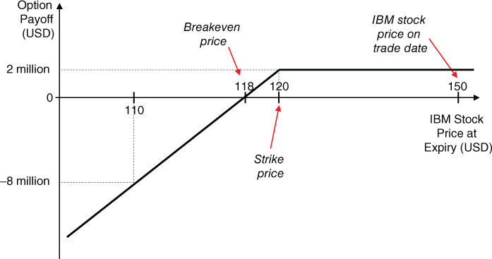
Figure 4.12 Payoff to the seller of the put option.
4.4.3 Standard Foreign Exchange Options
Most FX instruments involve two currencies: a specific amount of one currency is paid (or received) in exchange for receiving (or paying) a specific amount of another currency. An interesting aspect of FX options is that they are simultaneously a call and a put option. If the FX option is a call on one currency, it is necessarily a put option on another currency. Accordingly, when entering into an FX option, the term “call” (or “put”) is accompanied by the currency for which the option is a call (or a put). For example, a EUR–USD option in which the option buyer benefits when the USD strengthens is simultaneously a USD call and a EUR put option. Likewise, a EUR–USD option in which the option buyer benefits when the USD weakens is simultaneously a USD put and a EUR call option.
As a first example, suppose that a European entity highly expects to sell a manufacturing plant to a US investor. The plant is expected to be sold for USD 100 million in 1 year. The entity is exposed to a declining USD relative to the EUR. Accordingly, the entity decides to hedge the FX risk arising from the highly expected sale by buying an option with the following characteristics:
| EUR call/USD put terms | |
| Buyer | European entity |
| Option type | EUR call/USD put |
| Expiry | 1 year |
| Notional | USD 100 million |
| Strike | 1.16 |
| Settlement | Cash settlement |
| Premium | EUR 1.8 million to be paid two business days after trade date |
As this option is cash settled, the option will pay a EUR amount at expiry only when the option ends up being in-the-money (i.e., when the EUR–USD FX rate is greater than 1.16). The cash settlement amount (i.e., the option payoff) at expiry is calculated according to the following formula:
Figure 4.13 shows the option's payoff (i.e., the settlement amount) as a function of the EUR USD spot rate at expiry, without taking into account the premium that the entity paid for the option.
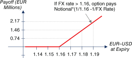
Figure 4.13 1.16 USD put/EUR call payoff at expiry (excluding premium).
On receipt of the USD 100 million, the entity will exchange the USD for EUR at the spot rate. The entity will also exercise the option at expiry when it ends up being in-the-money. The option payoff, if the option is exercised, will increase the EUR proceeds of the sale. Figure 4.14 shows the resulting EUR amount obtained through both transactions: the disposal of the plant and the option payoff. It can be observed that by purchasing the option the entity locked in a minimum EUR 86.2 million overall proceeds (excluding the option premium), while potentially receiving higher proceeds were the USD to strengthen relative to the EUR below 1.16.
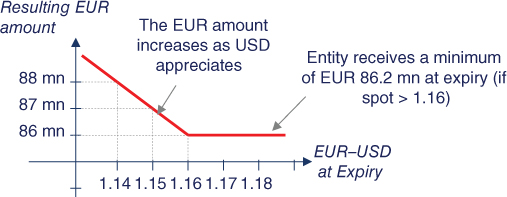
Figure 4.14 Option and plant disposal combined EUR amount (excluding premium).
As a second example, suppose that a European entity highly expects to purchase a machine from a US supplier. The machine is expected to cost USD 100 million. The invoice will be paid in USD in 1 year. The entity is exposed to a rising USD relative to the EUR. Accordingly, the entity decides to hedge the FX risk arising from the highly expected purchase by buying a EUR put/USD call option, whose main terms are as follows:
| EUR put/USD call terms | |
| Buyer | European entity |
| Option type | EUR put/USD call |
| Expiry | 1 year |
| Notional | USD 100 million |
| Strike | 1.16 |
| Settlement | Cash settlement |
| Premium | EUR 1.6 million to be paid two business days after trade date |
As this option is cash settled, the option will pay a EUR amount at expiry only when the option ends up being in-the-money (i.e., EUR–USD FX rate lower than 1.16). The cash settlement amount at expiry is calculated according to the following formula:
Figure 4.15 illustrates the option payoff (i.e., the settlement amount) as a function of the EUR–USD spot rate at expiry, excluding the premium that the entity paid for the option.

Figure 4.15 1.16 EUR put/USD call payoff at expiry (excluding premium).
At maturity of the transaction and in order to meet the USD 100 million payment, the entity will receive USD 100 million in exchange for a EUR amount at the spot rate prevailing on such date. The entity will also exercise the option when it ends up being in-the-money, decreasing the total EUR cost of the purchase. Figure 4.16 shows the resulting EUR amount from both transactions (excluding the option premium). It can be observed that by purchasing the EUR put, the entity limits the maximum EUR amount to be paid for the machine to EUR 86.2 million, while benefiting from a lower total payment were the EUR to appreciate above 1.16.
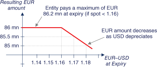
Figure 4.16 Option and machine purchase combined EUR amount (excluding premium).
Tunnel or Collar Combination
In the two previous examples, the entity paid a premium for the protection gained. It is more common, though, to buy an option and simultaneously sell the opposite option to avoid paying a premium. Applying this strategy to our second example, the entity would have bought the 1.16 EUR put and simultaneously sold a 1.26 EUR call. If we assume that the EUR call premium was also EUR 1.6 million, the entity neither paid nor received a premium for the combination of the two options. This strategy, called a zero-cost tunnel, is the most popular FX option hedging strategy. In our example, the purchased EUR put limits the maximum EUR amount to be paid for the machine to EUR 86.2 million. At the same time, the sold EUR call limits the minimum EUR amount to be paid to EUR 79.4 million (=100 million/1.26), as shown in Figure 4.17.
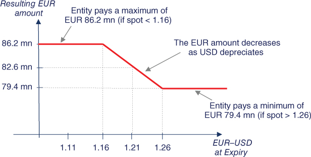
Figure 4.17 Option strategy and machine purchase combined EUR amount.
4.4.4 Interest Rate Options – Caps, Floors and Collars
When referring to interest rate options, the term cap is used instead of the term “call option”. Similarly, the term floor is used instead of the term “put option”. The reason for this is that a cap (floor) is in reality a string of call (put) options. For example, a borrower may prefer to pay a variable interest rate in a floating rate bond, but may require assurance that the interest payments do not exceed a maximum limit. An interest rate cap would achieve this objective by providing the issuer protection against rising interest rates. Usually, the borrower is not hedging only one interest payment but each interest payment on the bond. Therefore, a cap is in reality a string of options, each protecting a specific interest payment. Each option in a cap is called a caplet. Similarly, each option in a floor is called a floorlet.
Just as a borrower issuing a floating rate bond is concerned about rising interest rates, so an investor buying a floating rate bond is concerned about declining interest rates. An investor may prefer to receive a floating interest rate in a bond, but may require assurance that each interest receipt is not lower than a given minimum. An interest rate floor would achieve this objective by providing the issuer protection against low interest rates.
As an example, suppose that a borrower is about to issue a 5-year floating rate bond with an annual variable coupon of Euribor 12-month plus 50 basis points. The borrower expects interest rates to decline but wishes to be protected in case its view is wrong. As a result the borrower buys an interest rate cap. The cap provides protection when interest rates exceed 6%. The terms of the bond and the cap are summarised in the following tables:
| Bond terms | |
| Maturity | 5 years |
| Notional | EUR 100 million |
| Coupon | Euribor 12-month + 50 bps, to be paid annually |
| Interest rate cap terms | |
| Buyer | Borrower |
| Maturity | 5 years |
| Notional | EUR 100 million |
| Cap rate | 6% |
| Underlying | Euribor 12-month |
| Interest periods | Annual |
| Premium | EUR 2 million to be paid up-front |
In each interest period that the Euribor 12-month fixes above the 6% cap rate, the borrower will receive from the seller of the cap an amount related to the difference between the Euribor 12-month rate and the 6% cap rate. In each interest period that the Euribor 12-month is fixed at or below the 6% cap rate, the borrower will receive nothing. Figure 4.18 shows a caplet payoff as a function of the Euribor 12-month rate, without taking into account the cap premium.

Figure 4.18 Caplet payoff (excluding premium).
Figure 4.19 illustrates how the interest rate cap will operate in our example in conjunction with the bond. By entering into the cap, the borrower would achieve funding at a maximum rate of 6.50% (=6% + 0.50%), without taking into account the cap premium.
- On any interest reset date that Euribor 12-month is fixed at a rate above 6%, the borrower will receive through the cap the difference between Euribor 12-month and 6%. Because the borrower pays Euribor 12-month plus 50 basis points to the bondholders, the borrower will effectively pay a total interest of 6.50% (= Euribor 12M + 0.50% – (Euribor 12M – 6%)).
- On any interest reset date that Euribor 12-month is fixed below or at the 6% cap rate, the borrower will receive nothing through the cap. Therefore, the borrower will effectively pay an interest of Euribor 12-month rate plus the 50 basis points bond spread. This interest will be lower than 6.50%.
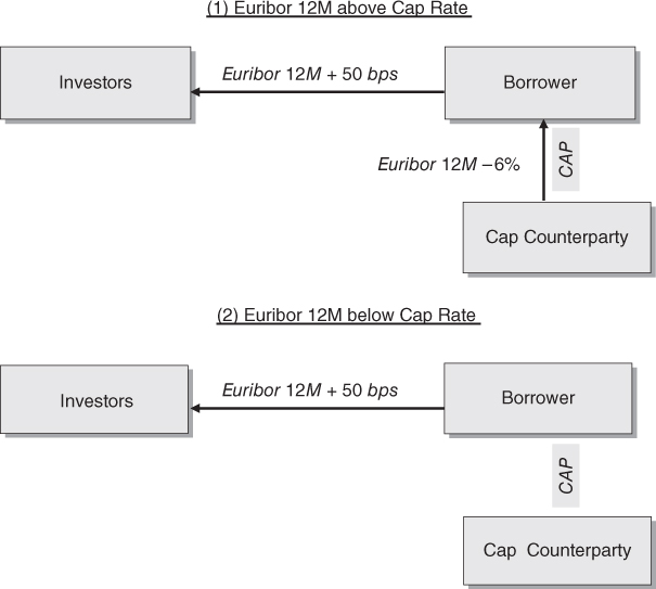
Figure 4.19 Floating rate bond and cap: combined interest cash flows (excluding premium).
Collar Strategy
Because the purchase of a cap requires the payment of an up-front premium, a cap is often transacted in conjunction with a floor to avoid making any up-front payments. The combination of a purchased cap and a sold floor is called a collar. In the case of a floating rate debt, a collar sets an upper and a lower limit on the interest a borrower would pay. If the premium of the cap is equal to the premium of the floor, the strategy is called a zero-cost collar, as no premium is exchanged at inception.
In our example, let us suppose that the borrower, in addition to buying the 6% cap, also sells a 4% floor. Through the floor, in each interest period that Euribor 12-month is fixed below 4%, the borrower will pay the floor buyer interest corresponding to the difference between the 4% and the Euribor 12-month rate (see Figure 4.20). In each interest period that Euribor 12-month is fixed at or above the 4% floor rate, the borrower will pay nothing.
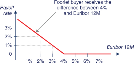
Figure 4.20 Floorlet payoff (excluding premium).
Figure 4.21 illustrates how the collar will operate in our example in conjunction with the debt. Through the collar, the borrower will achieve funding at a maximum rate of 6.50% (=6% + 0.50%) and at a minimum rate of 4.50% (=4% + 0.50%).
- On any interest reset date that Euribor 12-month fixes above 6%, the cap will be exercised and the borrower will effectively pay 6.50% (6% plus the 50 basis points bond spread).
- On any interest reset date that Euribor 12-month fixes between 4% and 6%, neither the cap nor the floor will be exercised. Thus, the borrower will pay the bond's Euribor 12-month rate plus 50 basis points spread coupon.
- On any interest reset date that Euribor 12-month fixes at a rate below 4%, the floor will be exercised. The borrower will pay the floor buyer the difference between 4% and Euribor 12-month. As a consequence, the borrower will effectively pay 4.50% (= Euribor 12M + 0.50% + 4% – Euribor 12M).
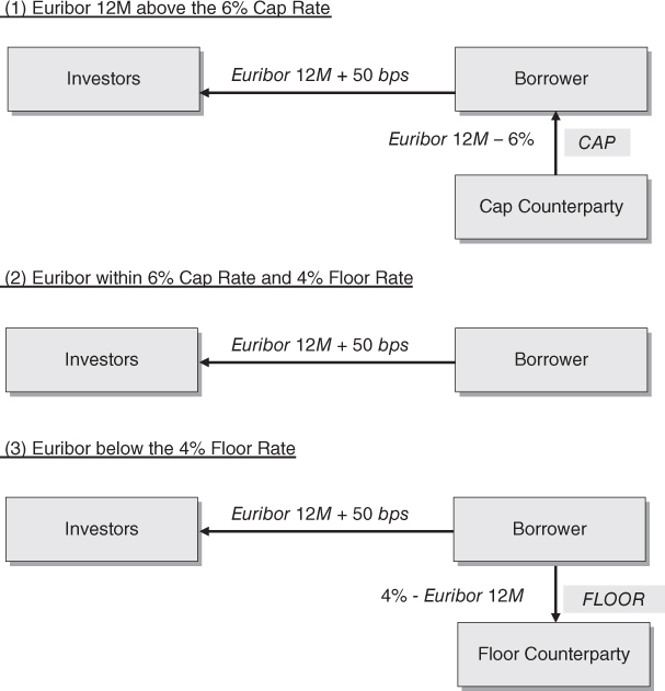
Figure 4.21 Floating rate bond and zero-cost collar: combined interest cash flows.
4.5 EXOTIC OPTIONS
It was mentioned above that there are two types of options: vanilla (or standard or regular) and exotic options. Vanilla options have all their terms fixed and predetermined at their start. Exotic options are any other options that are not considered vanilla options. In general, exotic options have at least one term (e.g., the strike) whose final value depends on specific conditions being met during their life. The rationale behind most exotic options is to have a lower premium than their vanilla equivalents.
It is not easy to classify the exotic options into a small number of groups because their characteristics are very wide-ranging. Also, it would be unrealistic to try to provide all the different exotic options being developed, as financial markets continuously come up with new ones. However, one possible categorisation is as follows:
- Path-dependent options. The payoff of a path-dependent option depends on how the underlying price (or rate) has traded over the life of the option. The most popular path-dependent options are average rate options, barrier options, and range accrual options. An average rate option, also called an “Asian option”, is an option whose payoff is determined by the average of its underlying price (or rate) during a pre-specified period of time before the option's expiry. Barrier options are the most popular exotic options, and I will cover them next. A range accrual option is an option whose payoff is determined by the number of days that the underlying stays within a specific range during a pre-specified period of time.
- Correlation options. The payoff of a correlation option is affected by more than one underlying. The most popular correlation options are basket options, quanto options and spread options. A basket option is an option on a portfolio of underlyings. A quanto option is an option whose payoff denominated in one currency while its underlying is denominated in another currency. A spread option is an option whose payoff is determined by the difference of two prices (or indices or rates).
- Other types of exotic options. This broad category groups all other options not included in the previous two categories. The most common options in this category are digital options. A digital option is an option whose payoff is either a fixed amount of cash (or other asset) or nothing.
4.6 BARRIER OPTIONS
The most popular type of exotic options are barrier options. Barrier options allow entities to tailor a hedging strategy to a very specific market view. The payoff of a barrier option depends on whether the price of the underlying crosses a given threshold, called the barrier, before maturity. Alternatively, in some barrier options the determination of whether the barrier has been crossed is determined only at maturity. I assume henceforth that the crossing of barrier is determined during the life of the option.
In general there are two types of barrier options: knock-in options and knock-out options:
- Knock-in options do not exist when traded and come into existence only when the price of the underlying reaches the barrier at any time during the life of the option.
- Knock-out options come out of existence when the price of the underlying reaches the barrier at any time during the life of the option.
The existence of the barrier lowers the probability of exercise, and therefore barrier options are cheaper than their vanilla counterparts. Thus, an entity that has a strong view about future movements on a specific FX rate can reduce its hedging costs by using barrier options, but it also needs to be prepared to assume the adverse consequences were its view wrong.
4.6.1 Knock-out Barrier Options – Product Description
A knock-out option at inception is a standard option. However, this option ceases to exist when its barrier is crossed. For example, imagine that a EUR-based USD exporter has the view that the EUR will strengthen against the USD over the next 6 months, while it expects the EUR not to appreciate beyond 1.28. The entity buys a 6-month EUR knock-out call with strike 1.16 and barrier 1.28. The premium of a knock-out option is lower than the premium of its equivalent standard option because the protection disappears when the 1.28 barrier is crossed.
- If the EUR–USD never trades at or above 1.28 during the life of the option, the entity effectively has protection identical to a standard option with strike 1.16 (see Figure 4.22).
- However, if at any time during the life of the option the 1.28 barrier is crossed, the option ceases to exist and the entity losses its protection (see Figure 4.23).
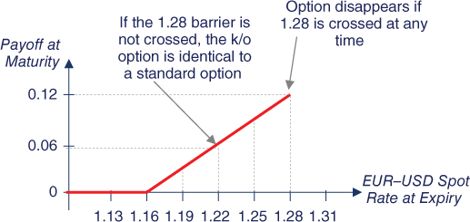
Figure 4.22 EUR knock-out call – barrier not hit: payoff at expiry (excluding premium).
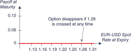
Figure 4.23 EUR knock-out call – barrier was hit: payoff at expiry (excluding premium).
4.6.2 Knock-in Barrier Options – Product Description
A knock-in option is an inactive option that automatically comes to life should the underlying rate trade at or beyond the barrier. For example, A EUR-based USD importer has the view that the EUR will weaken against the USD over the next 6 months, but expects the EUR to have a large movement beyond 1.05. The entity buys a 6-month EUR knock-in put with strike 1.15 and barrier 1.05. The premium of a knock-in option is lower than the premium of its equivalent standard option because there is protection only when the 1.05 barrier is crossed.
- If the EUR–USD exchange rate never trades at or below 1.05, the entity has no option – equivalent to the entity having no protection (see Figure 4.24).
- If the EUR–USD exchange rate trades at or below 1.05, the entity effectively has bought a standard option at substantial savings in option premium (see Figure 4.25).
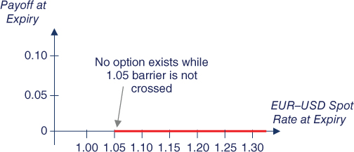
Figure 4.24 EUR knock-in put – barrier not hit: payoff at expiry (excluding premium).

Figure 4.25 EUR knock-in put – barrier was hit: payoff at expiry (excluding premium).
The two barrier options just covered are the most common ones, involving a single barrier. More complex barrier options can be obtained with double barriers that activate or extinguish an option if, for example, the two barriers are crossed during the life of the option. Also, in our example, the exchange rate was monitored continuously to check if the barrier was crossed. Some barrier options observe the barrier only on specific dates. In summary, many different variations of barrier options are available in the financial markets.
4.7 RANGE ACCRUALS
A range accrual option is an option that accrues value for each day that a reference rate remains within a specified range (the accrual range) during the accrual observation period. For example, suppose that an investor buys an accrual option on the Euro Stoxx 50 index (the reference rate). The option has 6 months to expiration and pays EUR 10,000 for each day that the index closes in the range 3,000 to 3,200 (the accrual range). The investor pays a EUR 600,000 premium for the option. There are 130 trading days in the accrual observation period. Therefore, for the investor to break even, the reference rate must trade within the accrual range for 60 days (=600,000/10,000), or 46% of the total trading days.
In the interest rates market, interesting alternatives to standard interest rate swaps are range accrual swaps. An example of a popular range accrual structure is the following. Suppose that a corporate wants to hedge its exposure to a 5-year EUR 100 million floating rate liability by paying a fixed rate of 4%, well below the market's 5% 5-year swap rate. Unlike a standard swap, the floating rate is conditional on how many days an observation rate (in our example the Euribor 12-month rate) is within a predefined range (e.g., 3.7–4.7%) in the interest period. The aim of the range accrual swap is to lower the fixed rate of the swap by assuming the risk that the Euribor 12-month rate fixes outside the accrual range. The interest flows are as follows (see Figure 4.26):
- The entity pays 4% annually, on EUR 100 million.
- The entity receives Euribor 12-month on the interest period's accrued nominal. The accrued nominal of an interest period is calculated using the formula
where n is number of fixings during the interest period that the Euribor 12-month is within the 3.70– 4.70% range, and N is the total number of fixings in the interest period.
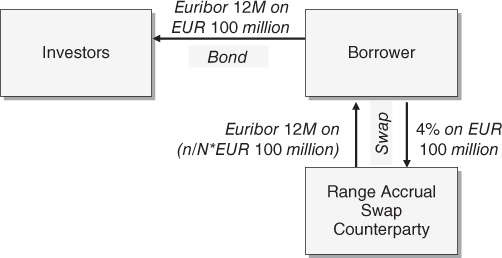
Figure 4.26 Range accrual – interest flows.
FX range accrual forwards are an alternative to hedging with FX forwards. For each of the daily fixings up to maturity that the FX spot rate remains within a predetermined range, the forward nominal accrues a certain amount at a forward rate. The accrual forward rate is a better than market rate. For example, suppose that a EUR-based USD exporter wants to hedge a USD 40 million sale expected to take place in 3 months. The exporter expects the EUR–USD spot rate to trade within the 1.23–1.26 range during the next 2 months. The EUR–USD 3-month FX forward is 1.2500. Instead of entering into a standard forward at 1.2500, the exporter enters into a range accrual forward at 1.2400 with the following accruing terms:
- Every day the EUR–USD spot rate falls within the 1.23–1.26 range, the accrued notional increases by USD 1 million.
- Every day the EUR–USD spot rate falls outside the 1.23–1.26 range, there are no accruals.
The accrual observation period has 65 observation days. The exporter expects that a total of 40 observation days the EUR–USD will close within the accrual range.
Suppose further that on 50 days, the EUR–USD spot rate remained within the 1.23–1.26 range. As a consequence, the exporter ended up with a contract to sell USD 50 million (=50 × 1 million) at a rate of 1.2400. The exporter then used the first USD 40 million of the range accrual forward to hedge the sale, but was left with a USD 10 million excess.