5.11 CASE STUDY: HEDGING A FORECAST SALE AND SUBSEQUENT RECEIVABLE WITH A KNOCK-IN FORWARD (INSTRUMENT IN ITS ENTIRETY)
In this section I will cover an approach to apply hedge accounting when (i) a knock-in forward is involved and (ii) the entity does not want to split the instrument (see previous section) for hedge accounting purposes due to its operational complexity.
5.11.1 Hedging Relationship Documentation
Under the approach covered in this section the hedging instrument would be the knock-in forward in its entirety. The hedged item was the cash flow stemming from the USD 100 million of a highly expected forecast sale (see previous cases). The risk management objective was to mitigate its variability against movements in the EUR–USD FX rate. ABC documented the hedging relationship as follows:
| Hedging relationship documentation | |
| Risk management objective and strategy for undertaking the hedge | The objective of the hedge is to protect the EUR value of the cash flow stemming from a USD 100 million highly expected sale of finished goods and its ensuing receivable against unfavourable movements in the EUR–USD exchange rate. This hedging objective is consistent with the entity's overall FX risk management strategy of reducing the variability of its profit or loss statement caused by purchases and sales denominated in foreign currency. The designated risk being hedged is the risk of changes in the EUR fair value of the highly expected cash flow |
| Type of hedge | Cash flow hedge |
| Hedged item | The cash flow stemming from a USD 100 million highly expected forecast sale of finished goods and its subsequent receivable, expected to be settled on 30 June 20X5. This sale is highly probable as similar transactions have occurred in the past with the potential buyer, for sales of similar size, and the negotiations with the buyer are at an advanced stage |
| Hedging instrument | The knock-in forward contract with reference number 014568. The main terms of the knock-in forward are a USD 100 million notional, a 1.2600 forward rate, a 1.1620 barrier, a 30 June 20X5 maturity and a physical settlement provision. The counterparty to the knock-in forward is XYZ Bank and the credit risk associated with this counterparty is considered to be very low |
| Hedge effectiveness assessment | See below |
5.11.2 Hedge Effectiveness Assessment
Hedge effectiveness will be assessed by comparing changes in the fair value of the hedging instrument in its entirety to changes in the fair value of a hypothetical derivative. The terms of the hypothetical derivative – a EUR–USD forward contract for maturity 30 June 20X5 with nil fair value at the start of the hedging relationship – reflected the terms of the hedged item. The terms of the hypothetical derivative are as follows:
| Hypothetical derivative – terms | |
| Start date | 1 October 20X4 |
| Counterparties | ABC and credit risk-free counterparty |
| Maturity | 30 June 20X5 |
| ABC sells | USD 100 million |
| ABC buys | EUR 79,872,000 |
| Forward Rate | 1.2520 (*) |
(*) Market credit risk-free forward rate for 30 June 20X5
Changes in the fair value of the hedging instrument will be recognised as follows:
- The effective part of the gain or loss on the hedging instrument will be recognised in the cash flow hedge reserve of OCI. The accumulated amount in equity will be reclassified to profit or loss in the same period during which the hedged expected future cash flow affects profit or loss, initially adjusting the sales amount when the sale is recognised and thereafter adjusting the revaluation of the receivable.
- The ineffective part of the gain or loss on the hedging instrument will be recognised immediately in profit or loss.
Hedge effectiveness will be assessed prospectively at hedging relationship inception, on an ongoing basis at least upon each reporting date and upon occurrence of a significant change in the circumstances affecting the hedge effectiveness requirements.
Hedge effectiveness assessment will be performed, and effective/ineffective amounts will be calculated, on a forward-forward basis. In other words, the forward element of both the hedging instrument and the hypothetical derivative will be included in the hedging relationship.
The hedging relationship will qualify for hedge accounting only if all the following criteria are met:
- The hedging relationship consists only of eligible hedge items and hedging instruments. The hedge item is eligible as it is a highly expected forecast transaction that exposes the entity to fair value risk, affects profit or loss and is reliably measurable. The hedging instrument is eligible as it is a derivative and it does not result in a net written option.
- At hedge inception there is a formal designation and documentation of the hedging relationship and the entity's risk management objective and strategy for undertaking the hedge.
- The hedging relationship is considered effective.
The hedging relationship will be considered effective if the following three requirements are met:
- There is an economic relationship between the hedged item and the hedging instrument.
- The effect of credit risk does not dominate the value changes that result from that economic relationship.
- The hedge ratio of the hedging relationship is the same as that resulting from the quantity of hedged item that the entity actually hedges and the quantity of the hedging instrument that the entity actually uses to hedge that quantity of hedged item. The hedge ratio should not be intentionally weighted to create ineffectiveness.
Whether there is an economic relationship between the hedged item and the hedging instrument will be assessed on a quantitative basis using the scenario analysis method for two scenarios in which the EUR–USD FX rate at the end of the hedging relationship (30 June 20X5) will be calculated by shifting the EUR–USD spot rate prevailing on the assessment date by ±10%, and the change in fair value of both the hedging instrument and the hedged item compared.
5.11.3 Hedge Effectiveness Assessment Performed at Hedge Inception
The hedging relationship was considered effective as the following three requirements were met:
- There was an economic relationship between the hedged item and the hedging instrument. Based on the quantitative assessment performed (see below), the entity concluded that the change in fair value of the hedged item was expected to be largely offset by the change in fair value of the hedging instrument, corroborating that both elements had values that would generally move in opposite directions.
- The effect of credit risk did not dominate the value changes resulting from that economic relationship as the credit ratings of both the entity and XYZ Bank were considered sufficiently strong.
- The hedge ratio of the hedging relationship was the same as that resulting from the quantity of hedged item that the entity actually hedged and the quantity of the hedging instrument that the entity actually used to hedge that quantity of hedged item. The hedge ratio was not intentionally weighted to create ineffectiveness.
A quantitative assessment was performed using the scenario analysis method in which the performance of the hedging instrument and the hedged item was assessed under two scenarios.
In a first scenario, a EUR–USD spot rate at the end of the hedging relationship (1.3585) was assumed by shifting the EUR–USD spot rate prevailing on the assessment date (1.2350) by +10%, as shown in the table below. Of note is that the hedged item was valued using forward rates (i.e., on a forward basis).
| Scenario analysis assessment | ||
| Hedging instrument | Hypothetical derivative | |
| Nominal USD | 100,000,000 | 100,000,000 |
| Forward rate | 1.2600 | 1.2520 |
| Nominal EUR | 79,365,000 | 79,872,000 |
| Nominal USD | 100,000,000 | 100,000,000 |
| Final rate | 1.3585 (1) | 1.3585 |
| Value in EUR | 73,611,000 (2) | 73,611,000 |
| Difference | 5,754,000 (3) | 6,261,000 |
| Discount factor | 1.0000 | 1.0000 |
| Final fair value | 5,754,000 (4) | 6,261,000 |
| Initial fair value | -0- | -0- |
| Fair value | 5,754,000 (5) | 6,261,000 |
| Degree of offset | 91.9% (6) | |
Notes:
(1) Assumed spot rate on hedging relationship end date (30 June 20X5)
(2) 100,000,000/1.3585
(3) 79,365,000 – 73,611,000
(4) 5,754,000 × 1.0000
(5) 5,754,000 – Nil
(6) 5,754,000/6,261,000
In a second scenario, a EUR–USD spot rate at the end of the hedging relationship (1.1115) was assumed by shifting the EUR–USD spot rate prevailing on the assessment date (1.2350) by –10% as shown in the table below. Under that scenario the 1.1620 barrier was reached and, as a result, the knock-in forward became a 1.2600 standard forward.
| Scenario analysis assessment | ||
| Hedging instrument | Hypothetical derivative | |
| Nominal USD | 100,000,000 | 100,000,000 |
| Forward rate | 1.2600 | 1.2520 |
| Nominal EUR | 79,365,000 | 79,872,000 |
| Nominal USD | 100,000,000 | 100,000,000 |
| Market rate | 1.1115 | 1.1115 |
| Value in EUR | 89,969,000 | 89,969,000 |
| Difference | <10,604,000> | <10,097,000> |
| Discount factor | 1.0000 | 1.0000 |
| Final fair value | <10,604,000> | <10,097,000> |
| Initial fair value | -0- | -0- |
| Fair value change | <10,604,000> | <10,097,000> |
| Degree of offset | 98.9% | |
Based on the results of the quantitative assessment, the change in fair value of the hedged item was expected to be largely offset by the change in fair value of the hedging instrument, corroborating that both elements have values that will generally move in opposite directions.
The hedge ratio was established at 1:1, resulting from the USD 100 million of hedged item that the entity actually hedged and the USD 100 million of the hedging instrument that the entity actually used to hedge that quantity of hedged item.
Another hedge assessment was performed on 31 December 20X4 (reporting date). That assessment was very similar to the one performed at inception and has been omitted to avoid unnecessary repetition. Similarly, the hedge ratio was assumed to be 1:1 on that assessment date.
Additional Comments
Under the second scenario, the downward movement of the FX rate was sufficiently large to trigger the knock-in feature. Otherwise, the degree of offset would have been very different, potentially endangering the economic relationship requirement.
5.11.4 Fair Valuations of Hedging Instrument and Hypothetical Derivative at the Relevant Dates
The actual spot and forward exchange rates prevailing at the relevant dates were as follows:
| Date | Spot rate at indicated date | Forward rate for 30-Jun-20X5 (*) | Discount factor for 30-Jun-20X5 |
| 1-Oct-20X4 | 1.2350 | 1.2500 | 0.9804 |
| 31-Dec-20X4 | 1.2700 | 1.2800 | 0.9839 |
| 31-Mar-20X5 | 1.2950 | 1.3000 | 0.9901 |
| 30-Jun-20X5 | 1.3200 | 1.3200 | 1.0000 |
(*) Credit risk-free forward rate
Fair Valuation of the Hedging Instrument (Knock-in Forward Contract in its Entirety)
The fair value calculation of the hedging instrument (i.e., the standard forward contract) at each relevant date was as follows (adding the standard forward and knock-out options fair values from the previous section):
| 1-Oct-20X4 | 31-Dec-20X4 | 31-Mar-20X5 | 30-Jun-20X5 | |
| Fair value | -0- | 1,910,000 | 2,777,000 | 3,607,000 |
| Fair value change (period) | — | 1,910,000 | 867,000 | 830,000 |
| Fair value change (cumulative) | — | 1,910,000 | 2,777,000 | 3,607,000 |
Fair Valuation of the Hypothetical Derivative
The fair value calculation of the hypothetical derivative at each relevant date was as follows:
| 1-Oct-20X4 | 31-Dec-20X4 | 31-Mar-X5 | 30-Jun-X5 | |
| Fair value | -0- | 1,719,000 (1) | 2,920,000 (2) | 4,114,000 (3) |
| Cumulative change | — | 1,719,000 | 2,920,000 | 4,114,000 |
Notes:
(1) (100 mn/1.2520 – 100 mn/1.2800) × 0.9839
(2) (100 mn/1.2520 – 100 mn/1.3000) × 0.9901
(3) (100 mn/1.2520 – 100 mn/1.3200) × 1.0000
5.11.5 Calculation of Effective and Ineffective Amounts
The calculation of the effective and ineffective amounts of the change in fair value of the hedging instrument was as follows:
| 31-Dec-20X4 | 31-Mar-20X5 | 30-Jun-20X5 | |
| Cumulative change in fair value of hedging instrument | 1,910,000 | 2,777,000 | 3,607,000 |
| Cumulative change in fair value of hypothetical derivative | 1,719,000 | 2,920,000 | 4,114,000 |
| Lower amount | 1,719,000 | 2,777,000 (1) | 3,607,000 |
| Previous cumulative effective amount | Nil | 1,719,000 (2) | 2,586,000 |
| Available amount | 1,719,000 | 1,058,000 (3) | 1,021,000 |
| Period change in fair value of hedging instrument | 1,910,000 | 867,000 (4) | 830,000 |
| Effective amount | 1,719,000 | 867,000 (5) | 830,000 |
| Ineffective amount | 191,000 | Nil (6) | Nil |
Notes:
(1) Lower of 2,777,000 and 2,920,000
(2) 1,719,000, the sum of all prior effective amounts
(3) 2,777,000 – 1,719,000
(4) Change in the fair value of the hedging instrument during the period (i.e., since the last fair valuation)
(5) Lower of 1,058,000 (available amount) and 867,000 (period change in fair value of hedging instrument)
(6) 867,000 (period change in fair value of hedging instrument) – 867,000 (effective part)
5.11.6 Accounting Entries
The required journal entries were as follows.
- To record the knock-in forward trade on 1 October, 20X4
No on-balance-sheet accounting entries were required as initial fair value of the knock-in forward was zero.
- To record the closing of the accounting period on 31 December 20X4
The change in fair value of the knock-in forward since the last valuation was a EUR 1,910,000 gain, of which EUR 1,719,000 was deemed to be effective and recorded in the cash flow hedge reserve of equity, while EUR 191,000 was deemed to be effective and recorded in profit or loss.
- To record the sale agreement on 31 March 20X5
The sale agreement was recorded at the spot rate prevailing on that date (1.2950). Therefore, the sale EUR proceeds were EUR 77,220,000 (=100 million/1.2950). Because the machinery sold was not yet paid, a receivable was recognised. Suppose that the machinery was valued at EUR 68 million in ABC's statement of financial position.
The change in fair value of the knock-in forward since the last valuation was a gain of EUR 867,000, deemed to be fully effective and recorded in the cash flow hedge reserve of OCI.
The recognition of the sales transaction in profit or loss caused the release to profit or loss of the EUR 2,586,000 deferred hedge results accumulated in OCI.
- To record the settlement of the receivable, the knock-in forward on 30 June 20X5
The receivable was revalued at the spot rate prevailing on this date, showing a loss of EUR 1,463,000 (=100 million/1.3200 – 100 million/1.2950).
The receivable was paid by the customer, and thus USD 100 million was received. The spot rate on payment date was 1.32, so the USD 100 million payment was valued at EUR 75,758,000 (=100 million/1.32).
The change in fair value of the knock-in forward since the last valuation was a gain of EUR 830,000, fully deemed to be effective and recorded in the cash flow hedge reserve of OCI.
The recognition of the receivable revaluation in profit or loss caused the reclassification of the EUR 830,000 amount in the cash flow hedge reserve to profit or loss.
The settlement of the knock-in forward resulted in the payment of USD 100 million cash in exchange for EUR 79,365,000, representing an additional EUR 3,607,000 relative to the amount that settled the receivable.
- The following table gives a summary of the accounting entries, excluding the entries related to the cost of goods sold.
Cash Knock-in forward Accounts receivable Cash flow hedge reserve Profit or loss 1-Oct-20X4 Knock-in forward trade 31 Dec-20X4 Knock-in forward revaluation 1,910,000 1,719,000 191,000 31-Mar-20X5 Knock-in forward revaluation 867,000 867,000 Reserve reclassification <2,586,000> 2,586,000 Sale shipment 77,220,000 77,220,000 30-Jun-20X5 Knock-in forward revaluation 830,000 830,000 Knock-in forward settlement 3,607,000 <3,607,000> Receivable revaluation <1,463,000> <1,463,000> Reserve reclassification <830,000> 830,000 Receivable settlement 75,758,000 <75,758,000> TOTAL 79,365,000 -0- -0- -0- 79,365,000 (1) Note: Total figures may not match the sum of their corresponding components due to rounding.
5.12 CASE STUDY: HEDGING A FORECAST SALE AND SUBSEQUENT RECEIVABLE WITH A KNOCK-IN FORWARD (REBALANCING APPROACH)
Suppose that ABC decided to consider the whole knock-in forward as one instrument and, from an accounting perspective, tried to designate it as the hedging instrument in a hedging relationship. In this section I will cover the rebalancing approach to the application of hedge accounting. This approach rebalances the hedge ratio to changes in the circumstances surrounding a hedging relationship. This approach was covered in Section 5.8 for a participating forward.
5.12.1 Quantity of Hedged Item Estimation
The rebalancing approach is an interesting alternative for the application of hedge accounting when exotic options are involved and either (i) it is not feasible a split of the derivative between a hedge accounting friendly part and an undesignated part or (ii) designating the derivative in its entirety results in economic assessments that are too dependent on the path followed by the underlying market variable. The rebalancing approach starts by estimating the quantity of hedged item that would be hedged with the quantity of derivative actually traded.
Previously, it was mentioned that our knock-in forward could be split into two contracts (see Figure 5.23): (i) an FX forward at 1.2600, and (ii) a purchased knock-out USD call option with a 1.2600 strike and a 1.1620 barrier. Let us analyse two extreme scenarios:
- The option was knocked out (i.e., the 1.1620 barrier was reached). The hedge would then consist of just a 1.2600 forward (i.e., a standard forward). The hedge ratio would be 1:1 as in order to hedge USD 100 million of the forecast sale ABC would use USD 100 million of the forward, because any change value of the sale would be almost fully offset by the change in the fair value of the resulting forward.
- The option had a very high probability of being exercised (i.e., the option had a short time to expiry, was in-the-money and the probability of reaching the barrier was very low). In this scenario, it is as if the knock-in forward never existed as the changes in fair value of the forward would be almost fully offset by the changes in fair value of the option. The hedge ratio would be almost 0:1 (i.e., as if the forecast sale was unhedged).
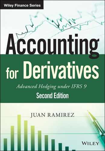
The quantity of hedged item (i.e., the forecast sale) could be viewed as the difference between the quantity of forward and the quantity of (knock-out) option:
The quantity of forward to be used by ABC was USD 100 million as its probability of being exercised was 100% (i.e., there is no optionality in a forward, and both parties will exchange the notional amounts at maturity).
Whilst the quantity of forward was known, the quantity of option to be used by ABC depended on its probability of being exercised –whether the barrier would not be reached before the end of the hedging relationship and whether the option would be in-the-money (i.e., when a EUR–USD spot rate lower than 1.2600 results at expiry). If both the option exists and it is in-the-money at expiry, ABC would fully exercise the option, which can be interpreted as ABC using a USD 100 million quantity of the option. Alternatively, if either (i) the 1.1620 barrier was reached during the option's life or (ii) the spot rate was at or above 1.2600 at expiry, ABC would not exercise the option, or in other words, ABC would not use any quantity of the option. Whilst ex ante ABC did not know whether the option would be exercised, the entity could estimate the option's probability of being exercised.
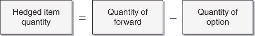
In order to have the appropriate hedge ratio, the quantity of hedged item to be used should equal the quantity of knock-in forward. As noted above, the quantity of knock-in forward is unknown at the commencement of the hedging relationship and can be estimated according to the following expression:
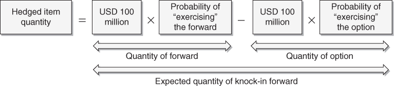
As mentioned previously, the quantity of forward was USD 100 million as the probability of “exercising” the forward was 100%. The probability of exercising an option can be approximated by its delta. Therefore, the quantity of hedged item can be estimated as:
The absolute value of an option's delta can be loosely interpreted as an approximate measure of the probability that it will expire in-the-money. If a knock-out option is very deep in-the-money and has a very low probability of reaching its barrier (i.e., it has a very high probability of being in-the-money at expiry), the absolute value of its delta will be close to 100%. Conversely, if a knock-out option is very deep out-of-the-money or it is close to its barrier (i.e., it has a low probability of being in-the-money at expiry), the absolute value of its delta will be close to zero. In our case, on 1 October 20X4 the delta of our knock-out option was 29%. The knock-out option delta as a function of the EUR–USD spot rate on that date had the profile depicted in Figure 5.26, showing that, for example, had the spot rate been 1.2600 the delta would have been 35%.
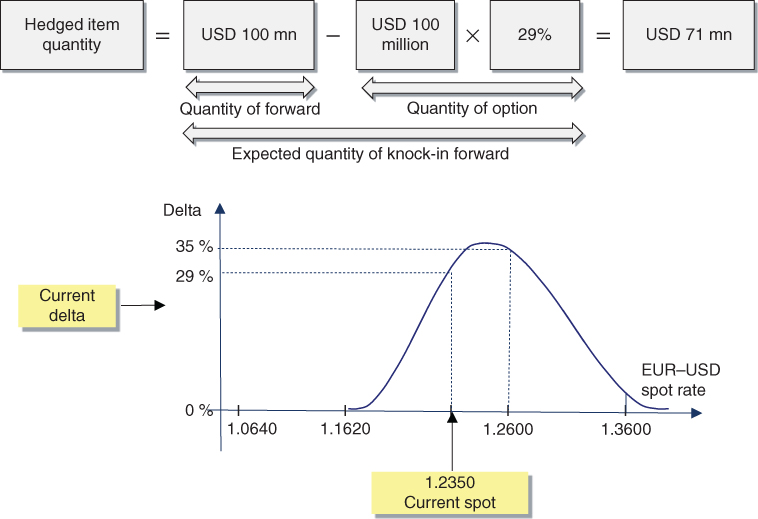
Figure 5.26 Option delta on 1 October 20X4.
As a result, the hedge ratio was established at 0.71:1, and USD 71 million of the hedged item was hedged using USD 100 million of the knock-in forward.
In our case, the hedging relationship would end on 30 June 20X5, when the knock-in forward contract matured (see Figure 5.27).
- Until 31 March 20X5, the effective parts of the changes in fair value of the knock-in forward would be recorded in OCI, while the ineffective parts would be recognised in profit or loss.
- On 31 March 20X5, the hedged cash flow (i.e., the sale) would be recognised in ABC's profit or loss and, simultaneously, cause the amounts previously recorded in equity (OCI) to be reclassified to profit or loss. Also on 31 March 20X5 a receivable denominated in USD would be recognised in ABC's statement of financial position.
- During the period from 31 March 20X5 until 30 June 20X5, the hedged item would be the USD accounts receivable resulting from the sale. This receivable would be revalued through profit or loss on 30 June 20X5.
- Also on 30 June 20X5, the effective part of the change in fair value of the knock-in forward would be recorded in OCI, while the ineffective part would be recognised in profit or loss. The amounts recognised in OCI would be reclassified to profit or loss, as the revaluation of the hedged item (i.e., the receivable) had impacted profit or loss. Therefore, there was no need to have a hedging relationship in place because already there would be an offset between the FX gains and losses on the revaluation of the USD accounts receivable and the revaluation gains and losses of the knock-in forward contract.
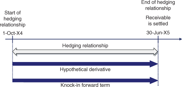
Figure 5.27 Hedge expected timeframe.
5.12.2 Hedging Relationship Documentation
At the inception of the hedging relationship, ABC documented the relationship as follows:
| Hedging relationship documentation | |
| Risk management objective and strategy for undertaking the hedge | The objective of the hedge is to protect the EUR value of a USD denominated cash flow stemming from a highly expected sale of finished goods and its ensuing receivable against movements in the EUR–USD exchange rate. This hedging objective is consistent with the entity's overall FX risk management strategy of reducing the variability of its profit or loss statement caused by purchases and sales denominated in foreign currency. The designated risk being hedged is the exchange rate risk attributable to movements in the EUR–USD exchange rate |
| Type of hedge | Cash flow hedge |
| Hedged item | The cash flow stemming from a USD 71 million sale of finished goods and its subsequent receivable, expected to be settled on 30 June 20X5. This sale is highly probable as similar transactions have occurred in the past with the potential buyer, for sales of similar size, and the negotiations with the buyer are at an advanced stage. The quantity of hedged item will be adjusted to incorporate changes in the hedge ratio |
| Hedging instrument | The knock-in forward contract with reference number 014565. The contract has a notional of USD 100 million, a 30 June 20X5 maturity, a 1.2600 forward rate and a 1.1620 barrier. The counterparty to the knock-in forward is XYZ Bank and the credit risk associated with this counterparty is considered to be very low |
| Hedge effectiveness assessment | See below |
5.12.3 Hedge Effectiveness Assessment
Hedge effectiveness will be assessed by comparing changes in the fair value of the hedging instrument to changes in the fair value of the hedged item.
The change in the fair value of the hedging instrument will be recognised as follows:
- The effective part of the gain or loss on the hedging instrument will be recognised in the cash flow hedge reserve of OCI. The accumulated amount in equity will be reclassified to profit or loss in the same period during which the hedged expected future cash flow affects profit or loss, adjusting the sales amount and thereafter the revaluation of the receivable.
- The ineffective part of the gain or loss on the hedging instrument will be recognised immediately in profit or loss.
Hedge effectiveness will be assessed prospectively at hedging relationship inception and on an ongoing basis at least upon each reporting date and upon occurrence of a significant change in the circumstances affecting the hedge effectiveness requirements.
The hedging relationship will qualify for hedge accounting only if all the following criteria are met:
- The hedging relationship consists only of eligible hedge items and hedging instruments. The hedge item is eligible as it is a highly expected forecast transaction that exposes the entity to fair value risk, is reliably measurable and affects profit or loss. The hedging instrument is eligible as it is a derivative and it does not result in a net written option.
- At hedge inception there is a formal designation and documentation of the hedging relationship and the entity's risk management objective and strategy for undertaking the hedge.
- The hedging relationship is considered effective.
The hedging relationship will be considered effective if the following three requirements are met:
- There is an economic relationship between the hedged item and the hedging instrument.
- The effect of credit risk does not dominate the value changes that result from that economic relationship.
- The hedge ratio of the hedging relationship is the same as that resulting from the quantity of hedged item that the entity actually hedges and the quantity of the hedging instrument that the entity actually uses to hedge that quantity of hedged item. The hedge ratio should not be intentionally weighted to create ineffectiveness.
Whether there is an economic relationship between the hedged item and the hedging instrument will be assessed on a quantitative basis using the scenario analysis method for four scenarios in which the EUR–USD FX rate at the end of the hedging relationship (30 June 20X5) will be calculated by shifting the EUR–USD spot rate prevailing on the assessment date by ±1 and ±0.5 standard deviations, and the changes in fair value of the hedging instrument with those of the hedging instrument compared.
5.12.4 Hedge Effectiveness Assessment Performed at Hedge Inception
The hedging relationship was considered effective as the following three requirements were met:
- There was an economic relationship between the hedged item and the hedging instrument.
- The effect of credit risk did not dominate the value changes resulting from that economic relationship as the credit ratings of both the entity and XYZ Bank were considered sufficiently strong.
- The hedge ratio of the hedging relationship was the same as that resulting from the quantity of hedged item that the entity actually hedged and the quantity of the hedging instrument that the entity actually used to hedge that quantity of hedged item. The hedge ratio was not intentionally weighted to create ineffectiveness.
An assessment was performed at hedge inception using the scenario analysis method for four scenarios, as follows. The EUR–USD spot rates at the end of the hedging relationship (30 June 20X5) for each scenario (1.1325, 1.1827, 1.2897 and 1.3467) were simulated by shifting the EUR–USD spot rate prevailing on the assessment date (1.2350) by ±1 and ±0.5 standard deviations, assuming a 10% volatility. In the case of ±1 standard deviations, the expression used to calculate the FX rates was:

As shown in the table below, the change in fair value of the hedged item was expected to be substantially offset by the change in fair value of the hedging instrument, corroborating that both elements had values that would generally move in opposite directions. The calculations related to the ±1 standard deviation shifts:
| –1 standard deviation | +1 standard deviation | ||||
| Hedging instrument (1) | Hedged item | Hedging instrument | Hedged item | ||
| Nominal USD | 100,000,000 | 71,000,000 | 71,000,000 | ||
| Hedged rate | 1.2600 | 1.2520 (2) | 1.2520 | ||
| Nominal EUR | 79,365,000 | 56,709,000 | 56,709,000 | ||
| Nominal USD | 100,000,000 | 71,000,000 | 71,000,000 | ||
| Final rate | 1.1325 | 1.1325 | 1.3467 | 1.3467 | |
| Value in EUR | 88,300,000 | 62,693,000 | 52,721,000 | ||
| Difference | <8,935,000> (3) | 5,984,000 | <3,988,000> (4) | ||
| Change in fair value | <8,935,000> | 5,984,000 | 5,109,000 (5) | <3,988,000> | |
Notes:
(1) The hedging instrument became a standard forward at 1.2600 as the embedded option was knocked out because the 1.1620 barrier was reached
(2) The credit risk-free forward rate for 30 June 20X5 prevailing at the start of the hedging relationship
(3) 79,365,000 – 88,300,000 = 100 mn/1.2600 – 100 mn/1.1325
(4) 52,721,000 – 56,891,000
(5) 100 mn/1.2600 – 100 mn/1.3467
The results of the quantitative assessments were as follows:
| Effectiveness assessment – scenario analysis results | |||||
| –1 standard deviation | –0.5 standard deviation | +0.5 standard deviation | +1 standard deviation | Total | |
| Final spot rate | 1.1325 | 1.1827 | 1.2897 | 1.3467 | |
| Change in fair value of hedging instrument | <8,935,000> | Nil (1) | 1,828,000 (2) | 5,109,000 | <1,998,000> |
| Change in fair value of hedged item | 5,802,000 | 3,141,000 (3) | <1,839,000> (4) | <4,170,000> | 2,934,000 |
| Degree of offset | 68.1% | ||||
Notes:
(1) The knock-in forward matured worthless as the EUR–USD spot rate ended up below 1.2600 and the barrier was assumed not to have been reached during the life of the instrument
(2) 100 mn/1.2600 – 100 mn/1.2897
(3) 71 mn/1.1827 – 71 mn/1.2480
(4) 71 mn/1.2897 – 71 mn/1.2480
The overall degree of offset was notably different from the expected 100%, being insufficient to conclude that the economic relationship criterion was met. Several factors contributed to such a difference:
- The degree of offset was highly dependent on the EUR–USD spot rate path simulated. If instead of four scenarios, ABC had simulated a large number of risk-neutral scenarios (e.g., a thousand) using a Monte Carlo simulation method (see Figure 5.28), the average degree of offset would have been close to 100%.
- The four scenarios used were not risk-neutral: the probability of a spot rate being shifted by, for example, +1 standard deviation is much lower than for a shift by +0.5 standard deviations. The degree of offsets should have been weighted by their probability of occurring.
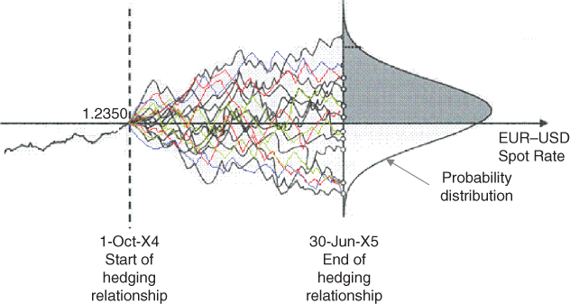
Figure 5.28 Spot rate simulation using Monte Carlo.
Suppose that a more robust Monte Carlo analysis resulted in an overall degree of offset much closer to 100% and that, as a result, ABC concluded that the change in fair value of the hedged item was expected to largely be offset by the change in fair value of the hedging instrument, corroborating that both elements had values that would generally move in opposite directions.
As calculated previously, the hedge ratio was established at 0.71:1, resulting from the USD 71 million of hedged item that the entity actually hedged and the USD 100 million of the hedging instrument that the entity actually used to hedge that quantity of hedged item.
Another hedge assessment was performed on 31 December 20X4 (reporting date). This assessment was very similar to the one performed at inception and has been omitted to avoid unnecessary repetition. I assume that the hedge ratio was set at 0.76:1. As a result the quantity of hedged item changed to USD 76 million.
The hedge ratio was also estimated on 31 March 20X5, resulting in 0.95:1. As a result the quantity of hedged item changed to USD 95 million.
5.12.5 Fair Valuations at the Relevant Dates
The fair values of the knock-in forward (see Section 5.11) at each relevant date were as follows:
| 1-Oct-20X4 | 31-Dec-20X4 | 31-Mar-X5 | 30-Jun-X5 | |
| Knock-in forward fair value | -0- | 1,910,000 | 2.777,000 | 3,607,000 |
| Cumulative change | -0- | 1,910,000 | 2.777,000 | 3,607,000 |
| Period change | — | 1,910,000 | 867,000 | 830,000 |
The fair values of the hedged item at each relevant date were as follows:
| 1-Oct-20X4 | 31-Dec-20X4 | 31-Mar-X5 | 30-Jun-X5 | |
| Hedged item quantity | 71 mn | 76 mn | 95 mn | — |
| Hedged item fair value | -0- | <1,221,000> (1) | <2,219,000> (2) | <3,909,000> (3) |
| Cumulative change | — | <1,221,000> | <2,219,000> | <3,909,000> |
Notes:
(1) (71 mn/1.2800 – 71 mn/1.2520) × 0.9839
(2) (76 mn/1.3000 – 76 mn/1.2520) × 0.9901
(3) (95 mn/1.3200 – 95 mn/1.2520) × 1.0000
5.12.6 Effective and Ineffective Amounts at the Relevant Dates
The calculation of the effective and ineffective amounts of the change in fair value of the hedging instrument was as follows:
| 31-Dec-20X4 | 31-Mar-20X5 | 30-Jun-20X5 | |
| Cumulative change in fair value of hedging instrument | 1,910,000 | 2,777,000 | 3,607,000 |
| Cumulative change in fair value of hedged item (opposite sign) | 1,221,000 | 2,219,000 | 3,909,000 |
| Lower amount | 1,221,000 | 2,219,000 (1) | 3,607,000 |
| Previous cumulative effective amount | Nil | 1,221,000 (2) | 2,088,000 |
| Available amount | 1,221,000 | 998,000 (3) | 1,519,000 |
| Period change in fair value of hedging instrument | 1,910,000 | 867,000 (4) | 830,000 |
| Effective amount | 1,221,000 | 867,000 (5) | 830,000 |
| Ineffective amount | 689,000 | Nil (6) | Nil |
Notes:
(1) Lower of 2,777,000 and 2,219,000
(2) Nil + 1,221,000, the sum of all prior effective amounts
(3) 2,219,000 – 1,221,000
(4) Change in the fair value of the hedging instrument during the period (i.e., since the last fair valuation)
(5) Lower of 998,000 (available amount) and 867,000 (period change in fair value of hedging instrument)
(6) 867,000 (period change in fair value of hedging instrument) – 867,000 (effective part)
5.12.7 Accounting Entries
The required journal entries were as follows.
- To record the knock-in forward contract trade on 1 October 20X4
No entries in the financial statements were required as the fair value of the knock-in forward contract was zero.
- To record the closing of the accounting period on 31 December 20X4
The change in fair value of the knock-in forward since the last valuation was a EUR 1,910,000 gain, of which the effective part was EUR 1,221,000 and recorded in OCI, and the ineffective part was EUR 689,000 and recorded in profit or loss.
- To record the sale agreement and the end of the hedging relationship on 31 March 20X5
The sale agreement was recorded at the EUR–USD spot rate prevailing on the date the sales are recognised (1.2950). Therefore, the sales EUR amount was EUR 77,220,000 (=100 million/1.2950). Because the machinery sold was not paid, a receivable was recognised. Suppose that the machinery was valued at EUR 68 million in ABC's statement of financial position.
The change in the fair value of the knock-in forward since the last valuation was a gain of EUR 867,000, fully effective and recorded in OCI. No ineffectiveness was present.
The recognition of the sales transaction in profit or loss caused the release to profit or loss of the EUR 2,088,000 deferred hedge results accumulated in OCI.
- To record the settlement of the receivable and the knock-in forward on 30 June 20X5
The receivable was revalued at the spot rate prevailing on this date, showing a loss of EUR 1,463,000 (=100 million/1.3200 – 100 million/1.2950).
The receivable was paid by the customer, and thus USD 100 million was received. The spot rate on payment date was 1.32, so the USD 100 million payment was valued at EUR 75,758,000 (=100 million/1.32).
The change in fair value of the knock-in forward since the last valuation was a gain of EUR 830,000, fully deemed to be effective and recorded in the cash flow hedge reserve of OCI.
The recognition of the receivable revaluation in profit or loss caused the recycling of the EUR 830,000 amount in the cash flow hedge reserve to profit or loss.
The settlement of the knock-in forward resulted in the payment of USD 100 million cash in exchange for EUR 79,365,000, representing an additional EUR 3,607,000 relative to the amount that settled the receivable.
The following table gives a summary of the accounting entries, excluding the entries related to the cost of goods sold:
| Cash | Knock-in forward | Accounts receivable | Cash flow hedge reserve | Profit or loss | |
| 1-Oct-20X4 | |||||
| Knock-in forward trade | |||||
| 31 Dec-20X4 | |||||
| Knock-in forward revaluation | 1,910,000 | 1,221,000 | 689,000 | ||
| 31-Mar-20X5 | |||||
| Knock-in forward revaluation | 867,000 | 867,000 | |||
| Reserve reclassification | <2,088,000> | 2,088,000 | |||
| Sale shipment | 77,220,000 | 77,220,000 | |||
| 30-Jun-20X5 | |||||
| Knock-in forward revaluation | 830,000 | 830,000 | |||
| Knock-in forward settlement | 3,607,000 | <3,607,000> | |||
| Receivable revaluation | <1,463,000> | <1,463,000> | |||
| Reserve reclassification | <830,000> | 830,000 | |||
| Receivable settlement | 75,758,000 | <75,758,000> | |||
| TOTAL | 79,365,000 | -0- | -0- | -0- | 79,365,000 |
(1) Note: Total figures may not match the sum of their corresponding components due to rounding.
5.13 CASE STUDY: HEDGING A HIGHLY EXPECTED FOREIGN SALE WITH A KIKO FORWARD
In previous cases I have analysed a hedging strategy that involved a knock-in forward, an instrument built with a barrier option. I now turn to another popular instrument, a knock-in knock-out forward (KIKO forward), also built with barrier options: a knock-out option and a knock-in option with identical strikes. In this section I will cover how a KIKO could be split to make part of it eligible for hedge accounting, and how the split affects the accounting treatment of the hedge strategy.
The risk being hedged in this case is the same as in the previous cases. Suppose that on 1 October 20X4 ABC Corporation, a company whose functional currency was the EUR, was expecting to sell finished goods to a US client. The sale was expected to occur on 31 March 20X5, and its related sale receivable was expected to be settled on 30 June 20X5. Sale proceeds were expected to be USD 100 million, to be received in USD.
ABC was interested in entering into an FX forward, but wanted to improve the forward rate by incorporating its view regarding the EUR–USD exchange rate during the next 9 months. ABC forecasted that a potential USD appreciation was going to be quite limited, not reaching below 1.1000. At the same time, ABC had the view that a potential USD depreciation above 1.3500 was unlikely. As a consequence, on 1 October 20X4 ABC entered into a KIKO forward that was obtained by combining the purchase of a knock-out USD put and a written knock-in USD call with the following terms:
| Knock-out USD put terms | Knock-in USD call terms | |||
| Trade date | 1 October 20X4 | Trade date | 1 October 20X4 | |
| Option buyer | ABC | Option buyer | XYZ Bank | |
| Option seller | XYZ Bank | Option seller | ABC | |
| USD notional | USD 100 million | USD notional | USD 100 million | |
| Strike | 1.2300 | Strike | 1.2300 | |
| Barrier | 1.3500 | Barrier | 1.1000 | |
| EUR notional | EUR 81,301,000 | EUR notional | EUR 81,301,000 | |
| Expiry date | 30 June 20X5 | Expiry date | 30 June 20X5 | |
| Knock-out provision | Option ceases to exist if at any time until expiry date the EUR–USD spot exchange rate trades at, or above, the barrier | Knock-in provision | Option can only be exercised if at any time until expiry date the EUR–USD spot exchange rate trades at, or below, the barrier | |
| Settlement | Physical delivery | Settlement | Physical delivery | |
| Premium | EUR 850,000 | Premium | EUR 850,000 | |
| Premium payment date | 1 October 20X4 | Premium payment date | 1 October 20X4 | |
There were four scenarios depending on the behaviour of the EUR–USD spot rate during the life of the KIKO forward:
| 1.10 barrier | 1.35 barrier | Equivalent position | Comments |
| Not hit | Not hit | Purchased 1.2300 USD put | Best scenario. ABC had protection and participated in USD appreciation |
| Hit | Not hit | 1.2300 forward | Good scenario. ABC ended up with a forward rate better than market forward (market forward would have been 1.2500) |
| Not hit | Hit | No derivative | Bad scenario. ABC ended up having no hedge in place |
| Hit | Hit | Written 1.2300 USD call | Worst scenario. ABC lost its protection and could not benefit from a USD appreciation |
Graphically, the KIKO payoff at expiry in each of the four scenarios is shown in Figure 5.29. The combination of the hedging instrument payoff and the expected cash flow resulted in a EUR amount, to be received by ABC in exchange for the USD 100 million sale proceeds, that was dependent on the four potential scenarios, as shown in Figure 5.30.
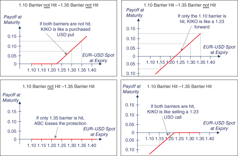
Figure 5.29 KIKO forward – scenarios.
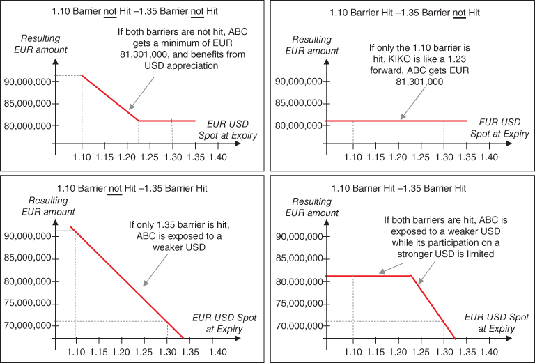
Figure 5.30 KIKO forward – resulting EUR amount.
5.13.1 Hedge Accounting Optimisation
One of the main issues that ABC faced regarding the KIKO forward was how to split the instrument into two parts, a first part eligible for hedge accounting and a second part treated as undesignated, to minimise the overall impact on profit or loss volatility. ABC considered the following choices:
- Divide the KIKO into two contracts (see Figure 5.31): (i) a 1.2300 forward and (ii) a “residual” derivative.
- Divide the KIKO into two contracts (see Figure 5.32): (i) a USD put option with a 1.2300 strike and (ii) a “residual” derivative.
- Consider the KIKO in its entirety as eligible for hedge accounting, if the corresponding requirements were met.
- Consider the whole KIKO as undesignated.

Figure 5.31 KIKO forward approach 1 – forward plus residual derivative.

Figure 5.32 KIKO forward approach 2 – USD put option plus residual derivative.
Approach 1: Split KIKO Forward into a Forward and a Residual Derivative
Under this approach, ABC would divide the KIKO into two contracts (see Figure 5.31): (i) a 1.2300 forward and (ii) a “residual” derivative. The residual derivative would be a written knock-in USD put with a 1.2300 strike and a 1.3500 barrier, and a purchased knock-out USD call with a 1.2300 strike and a 1.1100 barrier. The forward would be considered eligible for hedge accounting while the residual derivative would be considered as undesignated (i.e., speculative). Therefore, all the changes in the fair value of the residual derivative would be recorded in profit or loss. This approach would be recommended were ABC to believe that the 1.1000 barrier was more likely to be crossed than the 1.3500 barrier. One of the strengths of this approach was that the hedge effective part was recognised in the “sales” line of profit or loss.
Approach 2: Split KIKO Forward into an Option and a Residual Derivative
Under this approach, ABC would divide the KIKO into two contracts (see Figure 5.32): (i) a standard USD put option with a 1.2300 strike and (ii) a “residual” derivative. The residual derivative would be the combination of (i) a written knock-in USD put with a 1.2300 strike and a 1.3500 barrier, and (ii) a written knock-in USD call with a 1.2300 strike and a 1.1100 barrier. The standard USD put option would be considered eligible for hedge accounting and the residual derivative would be considered as undesignated (i.e., speculative). Therefore, all the changes in the fair value of the residual derivative would be recorded in profit or loss. This approach would be recommended if ABC estimated that it was very unlikely that either the 1.1000 barrier or the 1.3500 barrier would be crossed. One of the strengths of this approach was that the hedge effective part was recognised in the “sales” line of profit or loss.
Approach 3: Designate the KIKO Forward in its Entirety as Hedging Instrument
Under this approach, ABC would designate the KIKO forward in its entirety as the hedging instrument in a hedging relationship. This approach is, in my view, quite challenging to apply. The hypothetical derivative would be a 1.2480 forward. It was observed in our previous case – a hedge with a knock-in forward – that, whilst it was a “genuine” hedge strategy because there was a hedge in place in any EUR–USD scenario, it was relatively complex to justify that there was an economic relationship between the hedged item and the derivative that gave rise to offset, due to a volatile hedge ratio. A KIKO forward is even more challenging to justify that an economic relationship between this instrument and the hedged item, especially when the EUR–USD spot rate is near the 1.35 barrier. Moreover, once the 1.35 barrier is reached, there will be no hedge in place triggering an early termination of the hedging relationship.
Approach 4: Do Not Apply Hedge Accounting
Under this approach, ABC would consider the whole KIKO as undesignated. In other words, hedge accounting would not be applied. As a consequence, all changes in fair value of the KIKO would be recorded in profit or loss. Whilst this approach was the simplest from an operational perspective, saving the operational effort in complying with hedge accounting, it could notably increase profit or loss volatility. This approach was discarded by ABC.
The following table summarises these four choices:
| Approach | Hedging instrument | Hypothetical derivative | Comments |
| Split KIKO into standard forward and residual derivative | Standard forward | Standard forward | Recommended if probability of reaching the 1.10 barrier was notably greater than that of reaching the 1.35 barrier. Effective part of hedge recognised in “sales” line of profit or loss |
| Split KIKO into USD put and residual derivative | USD put | Standard forward | Recommended if it was unlikely that either the 1.10 barrier or 1.35 barrier would be crossed. Effective part of hedge and “aligned” time value recognised in “sales” line of profit or loss |
| Treat whole KIKO as designated | KIKO in its entirety | Standard forward | Challenging to prove economic relationship criterion. Hedging relationship would be terminated if 1.35 barrier is crossed |
| Treat whole KIKO as undesignated | N/A | N/A | Operationally, simplest approach, but two weaknesses: potential profit or loss volatility; and KIKO fair value changes not recognised in “sales” line of profit or loss |
5.13.2 Hedge Accounting Application for Approach 1 – Forward plus Residual Derivative
Suppose that ABC believed that the probability of crossing the 1.10 barrier was notably greater than that of crossing the 1.35 barrier. As a result, ABC selected the first approach, consisting of dividing the KIKO forward into two separate legal contracts: (i) a 1.2300 standard forward and (ii) a “residual” derivative.
The standard forward was designated as the hedging instrument in a cash flow hedging relationship. Hedge effectiveness was assessed by comparing the changes in fair value of the hedging instrument with the changes in fair value of a hypothetical derivative. The hypothetical derivative was a forward with zero initial fair value. The main terms of the actual forward (i.e., the hedging instrument) and the hypothetical derivative were as follows:
| Forward terms | Hypothetical derivative terms | |||
| Instrument | FX forward | Instrument | FX forward | |
| Start date | 1 October 20X4 | Start date | 1 October 20X4 | |
| Counterparties | ABC and XYZ Bank | Counterparties | ABC and credit risk-free counterparty | |
| Maturity | 30 June 20X5 | Maturity | 30 June 20X5 | |
| ABC sells | USD 100 million | ABC sells | USD 100 million | |
| ABC buys | EUR 81,301,000 | ABC buys | EUR 79,872,000 | |
| Forward rate | 1.2300 | Forward rate | 1.2520 | |
| Initial fair value | EUR 850,000 | Initial fair value | Zero | |
5.13.3 Hedging Relationship Documentation
The hedging relationship documentation was very similar to that in Section 5.10.2. The only differences are the terms of the hedging instrument, so we omit the documentation to avoid unnecessary repetition.
5.13.4 Hedge Effectiveness Assessment Performed at Hedge Inception
The hedging relationship was considered effective as the following three requirements were met:
- There was an economic relationship between the hedged item and the hedging instrument.
- The effect of credit risk did not dominate the value changes resulting from that economic relationship as the credit ratings of both the entity and XYZ Bank were considered sufficiently strong.
- The hedge ratio of the hedging relationship was the same as that resulting from the quantity of hedged item that the entity actually hedged and the quantity of the hedging instrument that the entity actually used to hedge that quantity of hedged item. The hedge ratio was not intentionally weighted to create ineffectiveness.
Based on the results of the quantitative assessment performed, it was concluded that the hedging instrument and the hedged item had values that would generally move in opposite directions. The assessment consisted of two scenarios being analysed as follows.
A EUR–USD spot rate at the end of the hedging relationship (1.3585) was simulated by shifting the EUR–USD spot rate prevailing on the assessment date (1.2350) by +10%. As shown in the table below, the change in fair value of the hedged item was expected to be substantially offset by the change in fair value of the hedging instrument, corroborating that both elements had values that would generally move in opposite directions.
| First scenario analysis assessment | ||
| Hedging instrument | Hypothetical derivative | |
| Nominal USD | 100,000,000 | 100,000,000 |
| Forward rate | 1.2300 | 1.2520 |
| Nominal EUR | 81,301,000 | 79,872,000 |
| Nominal USD | 100,000,000 | 100,000,000 |
| Forward rate | 1.3585 (1) | 1.3585 |
| Value in EUR | 73,611,000 (2) | 73,611,000 |
| Final fair value | 7,690,000 (3) | 6,261,000 |
| Initial fair value | 850,000 | -0- |
| Fair value change (cumulative) | 6,840,000 (4) | 6,261,000 |
| Degree of offset | 109.2% (5) | |
Notes:
(1) Assumed spot rate on hedging relationship end date
(2) 100,000,000/1.3585
(3) 81,301,000 – 73,611,000
(4) 7,690,000 – 850,000
(5) 6,840,000/6,261,000
In a second scenario, a EUR–USD spot rate at the end of the hedging relationship (1.1115) was assumed by shifting the EUR–USD spot rate prevailing on the assessment date (1.2350) by –10% as shown in the table below. Under that scenario I assume that the 1.1000 barrier was not reached.
| Second scenario analysis assessment | ||
| Hedging instrument | Hypothetical derivative | |
| Nominal USD | 100,000,000 | 100,000,000 |
| Forward rate | 1.2300 | 1.2520 |
| Nominal EUR | 81,301,000 | 79,872,000 |
| Nominal USD | 100,000,000 | 100,000,000 |
| Market rate | 1.1115 | 1.1115 |
| Value in EUR | 89,969,000 | 89,969,000 |
| Difference | <8,668,000> | <10,097,000> |
| Initial fair value | 850,000 | -0- |
| Fair value change | <9,518,000> | <10,097,000> |
| Degree of offset | 94.3% | |
The hedge ratio was established at 1:1, resulting from the USD 100 million of hedged item that the entity actually hedged and the USD 100 million of the hedging instrument that the entity actually used to hedge that quantity of hedged item.
Another hedge assessment was performed on 31 December 20X4 (reporting date). This assessment was very similar to the one performed at inception and has been omitted to avoid unnecessary repetition. Additionally, the hedge ratio was assumed to be 1:1 on that assessment date.
5.13.5 Fair Valuations of Derivative Contracts and Hypothetical Derivative at the Relevant Dates
The actual spot and forward exchange rates prevailing at the relevant dates were as follows (I assumed that on 15-Nov-20X4 the 1.1000 barrier was reached):
| Date | Spot rate at indicated date | Forward rate for 30-Jun-20X5 (*) | Discount factor for 30-Jun-20X5 |
| 1-Oct-20X4 | 1.2350 | 1.2480 | 0.9804 |
| 15-Nov-X4 | 1.0900 | 1.1000 barrier was crossed | |
| 31-Dec-20X4 | 1.2700 | 1.2800 | 0.9839 |
| 31-Mar-20X5 | 1.2950 | 1.3000 | 0.9901 |
| 30-Jun-20X5 | 1.3200 | 1.3200 | 1.0000 |
(*) Credit risk-free forward rate
Fair Valuation of the Hedging Instrument (Forward Contract)
The fair value calculation of the hedging instrument (i.e., the forward contract) at each relevant date was as follows:
| 1-Oct-20X4 | 31-Dec-20X4 | 31-Mar-20X5 | 30-Jun-20X5 | |
| Nominal EUR | 81,301,000 | 81,301,000 | 81,301,000 | 81,301,000 |
| Nominal USD | 100,000,000 | 100,000,000 | 100,000,000 | 100,000,000 |
| Forward rate for 30-Jun-20X5 | /1.2480 | /1.2800 | /1.3000 | /1.3200 |
| Value in EUR | 80,128,000 | 78,125,000 | 76,923,000 (1) | 75,758,000 |
| Difference | 1,173,000 | 3,176,000 | 4,378,000 (2) | 5,543,000 |
| Discount factor | × 0.9804 | × 0.9839 | × 0.9901 | × 1.0000 |
| Credit risk-free fair value | 1,150,000 | 3,125,000 | 4,335,000 (3) | 5,543,000 |
| CVA/DVA | <300,000> (4) | <5,000> | <2,000> | -0- |
| Fair value | 850,000 | 3,120,000 | 4,333,000 (5) | 5,543,000 |
| Fair value change (period) | — | 2,270,000 | 1,213,000 (6) | 1,210,000 |
| Fair value change (cumulative) | — | 2,270,000 | 3,483,000 (7) | 4,693,000 |
Notes:
(1) 100,000,000/1.3000
(2) 81,301,000 – 76,923,000
(3) 4,378,000 × 0.9901
(4) This figure includes a CVA as well as the bid/offer. The figure is relatively large due a substantial additional profit applied by XYZ Bank. ABC decided not to initially recognise any up-front loss on the trade
(5) 4,335,000 + <2,000>
(6) 4,333,000 – 3,120,000
(7) 4,333,000 – 850,000
Fair Valuation of the Hypothetical Derivative
The fair value calculation of the hypothetical derivative at each relevant date was as follows:
| 1-Oct-20X4 | 31-Dec-20X4 | 31-Mar-X5 | 30-Jun-X5 | |
| Fair value | -0- | 1,719,000 (1) | 2,920,000 (2) | 4,114,000 (3) |
| Cumulative change | — | 1,719,000 | 2,920,000 | 4,114,000 |
Notes:
(1) (100 mn/1.2520 – 100 mn/1.2800) × 0.9839
(2) (100 mn/1.2520 – 100 mn/1.3000) × 0.9901
(3) (100 mn/1.2520 – 100 mn/1.3200) × 1.0000
Fair Valuation of the Residual Derivative
The fair value of the knock-out option was computed using a closed-ended formula to value barrier options. Remember that all the change in the fair value of this option was recorded in profit or loss, as this option contract was undesignated.
On 15 November 20X4 the EUR–USD spot rate crossed the 1.1000 barrier. As a result, at that moment the knock-out USD call element of the residual derivative ceased to exist and the knock-in USD call of the KIKO became a standard USD call option from that date. The residual derivative fair value was calculated as follows:

The fair value of the residual derivative at each relevant date was as follows:
| 1-Oct-20X4 | 31-Dec-20X4 | 31-Mar-20X5 | 30-Jun-20X5 | |
| KIKO fair value (FV) | -0- | 2,188,000 | 1,450,000 | 5,543,000 |
| Forward fair value | 850,000 | 3,120,000 | 4,333,000 | 5,543,000 |
| Residual deriv. FV | <850,000> | <932,000> | <2,883,000> | -0- |
| Res. deriv. FV change | — | <82,000> | <1,951,000> | 2,883,000 |
Calculation of Effective and Ineffective Parts
The calculation of the effective and ineffective parts of the change in fair value of the hedging instrument was as follows:
| 31-Dec-20X4 | 31-Mar-20X5 | 30-Jun-20X5 | |
| Cumulative change in fair value of hedging instrument | 2,270,000 | 3,483,000 | 4,693,000 |
| Cumulative change in fair value of hypothetical derivative | 1,719,000 | 2,920,000 | 4,114,000 |
| Lower amount | 1,719,000 | 2,920,000 (1) | 4,114,000 |
| Previous cumulative effective amount | Nil | 1,719,000 (2) | 2,920,000 |
| Available amount | 1,719,000 | 1,201,000 (3) | 1,197,000 |
| Period change in fair value of hedging instrument | 2,270,000 | 1,213,000 (4) | 1,210,000 |
| Effective part | 1,719,000 | 1,201,000 (5) | 1,197,000 |
| Ineffective part | 551,000 | 12,000 (6) | 13,000 |
Notes:
(1) Lower of 3,483,000 and 2,920,000
(2) Nil + 1,719,000, the sum of all prior effective amounts
(3) 2,920 ,000 – 1,719,000
(4) Change in the fair value of the hedging instrument since the last fair valuation
(5) Lower of 1,201,000 (available amount) and 1,213,000 (period change in fair value of hedging instrument)
(6) 1,213,000 (period change in fair value of hedging instrument) – 1,201,000 (effective part)
5.13.6 Accounting Entries
The required journal entries were as follows.
- To record the forward and the residual derivative trades on 1 October, 20X4
At their inception, the fair values of the FX forward and the residual derivative were EUR 850,000 and <850,000>, respectively.
- To record the closing of the accounting period on 31 December 20X4
The change in fair value of the forward since the last valuation was a gain of EUR 2,270,000, of which EUR 1,719,000 was considered to be effective, and thus, recorded in the cash flow hedge reserve of OCI. The EUR 551,000 remainder represented the ineffective part, and was therefore recognised in profit or loss.
The change in fair value of the residual derivative since the last valuation was a EUR 82,000 loss, recognised in profit or loss as it was undesignated.
- To record the sale agreement on 31 March 20X5
The sale agreement was recorded at the spot rate prevailing on that date (1.2950). Therefore, the sale EUR proceeds were EUR 77,220,000 (=100 million/1.2950). Because the machinery sold was not yet paid, a receivable was recognised. Suppose that the machinery was valued at EUR 68 million in ABC's statement of financial position.
The change in fair value of the forward since the last valuation was a gain of EUR 1,213,000, of which EUR 1,201,000 was considered to be effective and recorded in the cash flow hedge reserve of OCI, while EUR 12,000 was considered to be ineffective and recorded in profit or loss.
The change in fair value of the residual derivative since the last valuation was a EUR 1,951,000 loss, recognised in profit or loss as it was undesignated.
The recognition of the sales transaction in profit or loss caused the release to profit or loss of the EUR 2,920,000 deferred hedge results accumulated in OCI.
- To record the settlement of the receivable and the forward on 30 June 20X5
The receivable was revalued at the spot rate prevailing on this date, showing a loss of EUR 1,463,000 (=100 million/1.3200 – 100 million/1.2950).
The receivable was paid by the customer, and thus USD 100 million was received. The spot rate on payment date was 1.32, so the USD 100 million payment was valued at EUR 75,758,000 (=100 million/1.32).
The change in the fair value of the forward since the last valuation was a gain of EUR 1,210,000, of which EUR 1,197,000 was considered to be effective and recorded in the cash flow hedge reserve of OCI, while EUR 13,000 was considered to be ineffective and recorded in profit or loss.
The settlement of the FX forward resulted in the payment of USD 100 million cash in exchange for EUR 81,301,000, representing an additional EUR 5,543,000 relative to the amount that settled the receivable.
The change in the fair value of the residual derivative since the last valuation was a gain of EUR 2,883,000. The residual derivative ended up worthless and, as a result, not exercised by either ABC or XYZ Bank.
The revaluation of the receivable in profit or loss caused the release to profit or loss of the EUR 1,197,000 deferred hedge results accumulated in OCI.
The following table gives a summary of the accounting entries, excluding the entries related to the cost of goods sold:
| Cash | Forward and residual derivative contracts | Accounts receivable | Cash flow hedge reserve | Profit or loss | |
| 1-Oct-20X4 | |||||
| Forward trade | <850,000> | 850,000 | |||
| Res. der. trade | 850,000 | <850,000> | |||
| 31 Dec-20X4 | |||||
| Forward revaluation | 2,270,000 | 1,719,000 | 551,000 | ||
| Res. der. revaluation | <81,000> | <81,000> | |||
| 31-Mar-20X5 | |||||
| Forward revaluation | 1,213,000 | 1,201,000 | 12,000 | ||
| Res. der. revaluation | <1,951,000> | <1,951,000> | |||
| Reserve reclassification | <2,920,000> | 2,920,000 | |||
| Sale shipment | 77,220,000 | 77,220,000 | |||
| 30-Jun-20X5 | |||||
| Forward revaluation | 1,210,000 | 1,197,000 | 13,000 | ||
| Res. der. revaluation | 2,883,000 | 2,883,000 | |||
| Forward settlement | 5,543,000 | <5,543,000> | |||
| Reserve reclassification settlement | <1,197,000> | 1,197,000 | |||
| Receivable revaluation | <1,463,000> | <1,463,000> | |||
| Receivable settlement | 75,758,000 | <75,758,000> | |||
| TOTAL | 81,301,000 | -0- | -0- | -0- | 81,301,000 |
(1) Note: Total figures may not match the sum of their corresponding components due to rounding.
5.13.7 Additional Remarks
Figure 5.33 summarises the effects of the strategy on ABC's profit or loss. The strategy worked very well. The total proceeds from the strategy were EUR 81,300,000, equivalent to a EUR–USD rate of 1.2300. Sales were translated at a 1.2478 rate. The strategy was successful in hedging the FX exposure because the 1.35 barrier was not crossed.
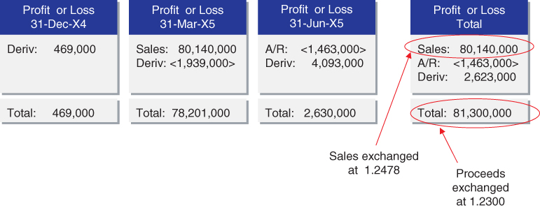
Figure 5.33 KIKO forward split into forward and residual derivative – effects on profit or loss.
Figure 5.34 illustrates the effects of the strategy on ABC's profit or loss, were the whole KIKO forward undesignated. All the change in fair value of the KIKO would have been recognised in profit or loss. The total proceeds from the strategy were EUR 81,300,000, equivalent to a EUR–USD rate of 1.2300. Sales were translated at a 1.2950 rate.

Figure 5.34 KIKO forward undesignated – effects on profit or loss.
The story would have been dramatically different had the 1.35 barrier been reached during the instrument's life. Suppose that the 1.35 barrier was crossed before the maturity of the KIKO forward (remember that the 1.1000 barrier was already crossed in November 20X4). At that moment the knock-in USD put embedded in the residual derivative would have been triggered, becoming a standard USD put with strike 1.2300. As a result, under the combination of the 1.2300 forward and the short position in the 1.2300 standard USD put, ABC would have been exposed to a rising EUR–USD rate while not being able to benefit from a declining EUR–USD rate below 1.2300. The total proceeds from the whole strategy would have been EUR 75,757,000, equivalent to a 1.3200 exchange rate.
5.14 CASE STUDY: HEDGING A FORECAST SALE AND SUBSEQUENT RECEIVABLE WITH A RANGE ACCRUAL (PART 1)
In this case study, I will analyse another popular hedging strategy, a range accrual forward. The case will show that the eligibility of this instrument for hedge accounting can be complex to demonstrate and that the hedge ratio is likely to need rebalancing at each reporting date.
The risk being hedged in this case is the same as in the previous cases. Suppose that on 1 October 20X4 ABC Corporation, a company whose functional currency was the EUR, was expecting to sell finished goods to a US client. The sale was expected to occur on 31 March 20X5, and the sale receivable was expected to be settled on 30 June 20X5. Sale proceeds were expected to be USD 100 million to be received in USD.
ABC had the view that the EUR–USD spot rate would remain within a 1.22–1.25 range during the next several months and wanted to benefit from a more attractive hedge were its view right. As a consequence, on 1 October 20X4, ABC entered into a range accrual forward with the following terms:
| FX range accrual terms | |
| Instrument | FX range accrual |
| Trade date | 1 October 20X4 |
| Counterparties | ABC and XYZ Bank |
| Maturity | 30 June 20X5 |
| ABC sells | USD nominal |
| ABC buys | EUR nominal, calculated as: USD nominal/Forward rate |
| USD nominal | USD 1,100,000 for each day that the reference rate fixes within the accrual range during the accruing period. Maximum USD nominal: USD 143 million |
| Accruing period | From, and including, 1 October 20X4 until, and including, 31 March 20X5 (a total of 130 fixings) |
| Accrual range | 1.22–1.25 |
| Reference rate | EUR–USD spot rate, European Central Bank fixing |
| Forward rate | 1.2300 |
| Settlement | Physical delivery |
| Initial fair value | Zero |
On 30 June 20X5, ABC would exchange for EUR an amount of USD equal to the USD nominal, at 1.2300. This rate was notably better than the 1.2500 rate that XYZ Bank quoted to ABC for a standard forward contract. To obtain such an advantageous rate, ABC ran the risk of an uncertain USD nominal. On 31 March 20X5, the USD notional was determined by observing the number of business days in the accruing period that the EUR–USD rate fixed within the 1.22–1.25 range (see Figure 5.35). Each observation within the range added USD 1.1 million to the USD notional.
- ABC expected the number of days with fixings within the range to be 91, and thus the USD nominal to be USD 100,100,000 (=91 days × 1.1 million). In other words, ABC expected the EUR–USD spot rate to stay within the range for 70% (=91 days/130 days) of the total period.
- A proportion higher than 70% (more than 91 days) would imply an overhedged position. ABC would probably need to unwind the excess, becoming exposed to a declining EUR–USD spot rate in relation to the amount to be unwound.
- A proportion lower than 70% (less than 91 days) would imply an underhedged position, exposing ABC to a rising EUR–USD exchange rate in relation to the underhedged amount.

Figure 5.35 Range accrual forward: resulting USD nominal.
One of the main issues that ABC faced regarding the range accrual forward was whether to split the instrument to minimise the overall impact on profit or loss volatility without substantially increasing operational complexity. ABC considered the following choices:
- to designate the range accrual in its entirety as the hedging instrument; and
- to split the range accrual into a standard forward (designated as hedging instrument) and a remaining derivative (undesignated).
5.15 CASE STUDY: HEDGING A FORECAST SALE AND SUBSEQUENT RECEIVABLE WITH A RANGE ACCRUAL (DESIGNATION IN ITS ENTIRETY)
In this section I assume that ABC decided to designate the whole range accrual forward as the hedging instrument. The main challenge was to determine whether there was an economic relationship between the hedged item and the range accrual that gave rise to offset. This required judgement, relying on a complex regression analysis.
Even if it was concluded that the hedge was eligible for hedge accounting, an unexpectedly volatile EUR–USD rate might add substantial mismatches between the hedged item and the hedging instrument, jeopardising any future hedge accounting designation for other range accruals the entity may enter into.
However, a range accrual forward is a genuine economic hedge and, in my opinion, entities should not be reluctant to enter into value added economic hedges because of a potentially unfavourable accounting treatment, unless operationally too costly.
5.15.1 Hedging Relationship Documentation
ABC denominated the range accrual contract as the hedging instrument in a foreign currency cash flow hedge, and the highly expected forecast sale as the hedged item. The hedging relationship would end on 30 June 20X5, when the range accrual matured (see Figure 5.36).
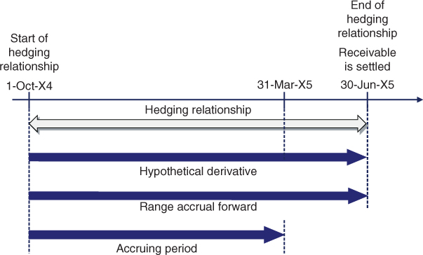
Figure 5.36 Hedging strategy timeframe.
ABC decided to base its assessment of hedge effectiveness on variations in forward FX rates. In other words, the forward points (i.e., the forward element) of the hypothetical derivative were included in the hedging relationship. ABC documented the hedging relationship as follows:
| Hedging relationship documentation | |
| Risk management objective and strategy for undertaking the hedge | The objective of the hedge is to protect the EUR value of a USD-denominated cash flow stemming from a highly expected sale of finished goods and its ensuing receivable against movements in the EUR–USD exchange rate. This hedging objective is consistent with the entity's overall FX risk management strategy of reducing the variability of its profit or loss statement caused by purchases and sales denominated in foreign currency. The designated risk being hedged is the exchange rate risk attributable to movements in the EUR–USD exchange rate |
| Type of hedge | Cash flow hedge |
| Hedged item | The cash flow stemming from a USD 100 million highly expected forecast sale of finished goods and its subsequent receivable, expected to be settled on 30 June 20X5. This sale is highly probable as similar transactions have occurred in the past with the potential buyer, for sales of similar size, and the negotiations with the buyer are at an advanced stage |
| Hedging instrument | The EUR–USD range accrual forward contract with reference number 014565. The counterparty to the contract is XYZ Bank and the credit risk associated with this counterparty is considered to be very low. The main terms are: a maturity on 30 June 20X5, a 1.2300 forward rate, a 1.22–1.25 accrual range observed up to the 31 March 20X5 and a USD 1.1 million notional for each business day that the spot EUR–USD is within the accrual range. |
| Hedge effectiveness assessment | See below |
5.15.2 Hedge Effectiveness Assessment
Hedge effectiveness will be assessed by comparing changes in the fair value of the hedging instrument in its entirety to changes in the fair value of a hypothetical derivative. The fair valuation of the hypothetical derivative will include both the forward and the spot elements. The terms of the hypothetical derivative – a EUR–USD forward contract for maturity 30 June 20X5 with nil fair value at the start of the hedging relationship – reflected the terms of the hedged item. The terms of the hypothetical derivative are as follows:
| Hypothetical derivative terms | |
| Instrument | FX forward |
| Start date | 1 October 20X4 |
| Counterparties | ABC and credit risk-free counterparty |
| Maturity | 30 June 20X5 |
| ABC sells | USD 100 million |
| ABC buys | EUR 79,872,000 |
| Forward rate | 1.2520 |
| Initial fair value | Zero |
Changes in the fair value of the hedging instrument will be recognised as follows:
- The effective part of the gain or loss on the hedging instrument will be recognised in the cash flow hedge reserve of OCI. The accumulated amount in equity will be reclassified to profit or loss in the same period during which the hedged expected future cash flow affects profit or loss, adjusting the sales amount or the revaluation of the receivable.
- The ineffective part of the gain or loss on the hedging instrument will be recognised immediately in profit or loss.
Hedge effectiveness will be assessed prospectively at hedging relationship inception and on an ongoing basis at least upon each reporting date and upon occurrence of a significant change in the circumstances affecting the hedge effectiveness requirements.
Hedge effectiveness assessment will be performed on a forward-forward basis. In other words, the forward element of the hypothetical derivative will be included in the assessment.
The hedging relationship will qualify for hedge accounting only if all the following criteria are met:
- The hedging relationship consists only of eligible hedge items and hedging instruments. The hedge item is eligible as it is a highly expected forecast transaction that exposes the entity to fair value risk through profit or loss and is reliably measurable. The hedging instrument is eligible as it is a derivative and it does not result in a net written option.
- At hedge inception there is a formal designation and documentation of the hedging relationship and the entity's risk management objective and strategy for undertaking the hedge.
- The hedging relationship is considered effective.
The hedging relationship will be considered effective if the following three requirements are met:
- There is an economic relationship between the hedged item and the hedging instrument.
- The effect of credit risk does not dominate the value changes that result from that economic relationship.
- The hedge ratio of the hedging relationship is the same as that resulting from the quantity of hedged item that the entity actually hedges and the quantity of the hedging instrument that the entity actually uses to hedge that quantity of hedged item. The hedge ratio should not be intentionally weighted to create ineffectiveness.
Whether there is an economic relationship between the hedged item and the hedging instrument will be assessed on a quantitative basis using a regression analysis method based on the EUR–USD FX rate during the previous 15 years and comparing the change in fair value of both the hypothetical derivative and the hedging instrument.
5.15.3 Hedge Effectiveness Assessment Performed at Hedge Inception
A regression analysis was performed on 1 October 20X4 to assess whether there is an economic relationship between the hedged item and the hedging instrument. The regression analysis was based on the EUR–USD FX rate actual performance during the previous 15 years and comparing the change in fair value of both the hypothetical derivative and the hedging instrument. The historical time horizon of 15 years was divided into 65 “simulation periods” of 9 months each. Each simulation period had an inception date and two subsequent balance sheet dates. In each simulation period, the behaviour of an equivalent hedging relationship using the historical data was simulated. Each observation pair (X, Y) was generated by computing the cumulative change in the fair value of a range accrual (variable X) and the cumulative change in fair value of a hypothetical derivative (observation Y), as shown in Figure 5.37. The terms of the range accrual and hypothetical derivative (accrual range and forward rates) were adjusted to conform to the market rates prevailing at the beginning of each simulation period. The results of the analysis were:
- A slope of 1.0. This was no coincidence as, prior to entering into the range accrual, its terms were designed to achieve such a slope.
- An R-squared of 82%.
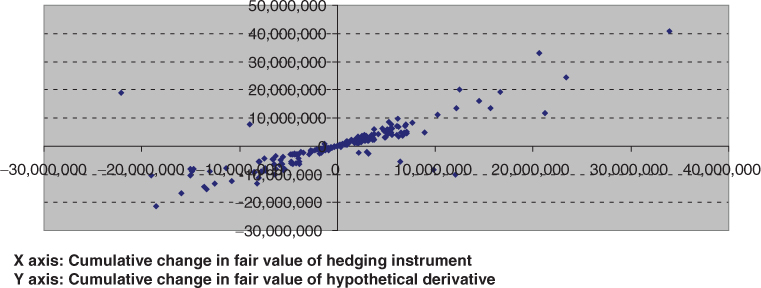
Figure 5.37 Range accrual – regression analysis.
The hedging relationship was considered effective as the following three requirements were met:
- There was an economic relationship between the hedged item and the hedging instrument. Based on the quantitative analysis performed, the entity concluded that the change in fair value of the hedged item was expected to be substantially offset by the change in fair value of the hedging instrument, corroborating that both elements had values that would generally move in opposite directions.
- The effect of credit risk did not dominate the value changes resulting from that economic relationship as the credit ratings of both the entity and XYZ Bank were considered sufficiently strong.
- The hedge ratio of the hedging relationship was the same as that resulting from the quantity of hedged item that the entity actually hedged and the quantity of the hedging instrument that the entity actually used to hedge that quantity of hedged item. The hedge ratio was not intentionally weighted to create ineffectiveness.
The hedge ratio was established at 1:1.43, based on the slope of the regression analysis. In other words, USD 100 million of hedged item was the quantity that the entity actually hedged and USD 143 million maximum USD notional was the quantity of the hedging instrument that the entity actually used to hedge that quantity of hedged item.
Another hedge assessment was performed on 31 December 20X4 (reporting date), when the EUR–USD spot rate was 1.2700. On that date, 66 days had already accrued within the accrual range, implying a minimum notional of USD 72.6 million. This assessment encompassed another regression in which each period already had 66 days accrued, 63 business days remaining to accrue and a relative position between the spot rate and the range accrual as shown in Figure 5.38. Suppose that after performing such regression its slope was 0.9, implying a 1:1.29 hedge ratio. In other words, USD 100 million of hedged item was the quantity that the entity actually hedged and USD 129 million maximum USD notional was the quantity of the hedging instrument that the entity actually used to hedge that quantity of hedged item. That hedge ratio meant that the hedging instrument represented 90% of the range accrual, while the 10% remainder was undesignated.
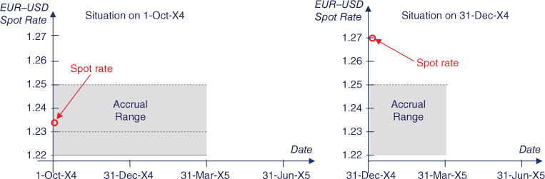
Figure 5.38 Range accrual – spot versus accrual range relative position.
5.15.4 Fair Valuations and Calculations of Effective/Ineffective Amounts
The behaviour of the EUR–USD spot rate during the life of the instrument is shown in Figure 5.39. The actual spot and forward exchange rates prevailing at the relevant dates were as follows:
| Date | Spot rate at indicated date | Accumulated number of days within range | USD nominal | Forward rate for 30-June-20X5 | Discount factor for 30-Jun-20X5 |
| 1-Oct-20X4 | 1.2350 | — | -0- | 1.2480 | 0.9804 |
| 31-Dec-20X4 | 1.2700 | 66 | 72,600,000 | 1.2800 | 0.9839 |
| 31-Mar-20X5 | 1.2950 | 100 | 110,000,000 | 1.3000 | 0.9901 |
| 30-Jun-20X5 | 1.3200 | — | 100,000,000 (1) | 1.3200 | 1.0000 |
Note:
(1) Assuming that an excess USD 10 million nominal was sold on 31-Mar-20X5 to eliminate the overhedged situation
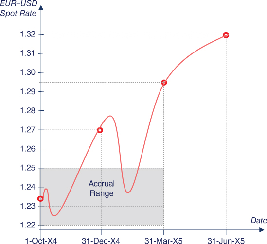
Figure 5.39 Behaviour of the EUR–USD spot rate during the hedging relationship term.
Fair Valuation of the Hedging Instrument and the Range Accrual Forward Contract
The following table shows the fair values of the range accrual forward contract and the hedging instrument at each relevant date. The fair values of the range accrual were calculated using a Monte Carlo model. As a result of the hedged ratio, the hedging instrument represented 100% (up to 31-Dec-20X4), 90% (from 31-Dec-20X4 to 31-Mar-20X5) and 100% (from 31-Mar-20X5 to 30-Jun-20X5 after an excess USD 10 million of the range accrual was sold) of the range accrual.
| 1-Oct-20X4 | 31-Dec-20X4 | 31-Mar-20X5 | 30-Jun-20X5 | |
| Range accrual fair value | -0- | 2,611,000 | 4,768,000 | 5,543,000 (1) |
| Range accrual fair value change (period) | — | 2,611,000 | 2,157,000 (2) | 1,208,000 (3) |
| Hedging instrument fair value | -0- | 2,611,000 | 4,291,000 (4) | 5,543,000 |
| Hedging instrument FV change (period) | — | 2,611,000 | 1,941,000 (5) | 1,208,000 |
| Hedging instrument FV change (cumulative) | — | 2,611,000 | 4,291,000 | 5,543,000 |
| Undesignated part FV | — | — | 477,000 (6) | — |
| Hedging instrument FV change (cumulative) | — | — | 216,000 (7) | — |
Notes:
(1) Taking into account that USD 10 million notional was sold on 31-Mar-20X5
(2) 4,768,000 – 2,611,000
(3) 5,543,000 – 4,335,000; relative to a valuation on 31-Mar-20X5 of EUR 4,335,000 (=4,768,000 – 433,000), to take into account the sale on that date
(4) 90% × 4,768,000 as after 31-Dec-X4 the hedging instrument was 90% of the range accrual
(5) 4,291,000 – 90% × 2,611,000
(6) 4,768,000 × 10%
(7) 477,000 – 10% × 2,611,000
On 31 March 20X5, ABC unwound the USD 10 million excess nominal in the market, receiving EUR 433,000.
Fair Valuation of the Hypothetical Derivative
The fair value calculation of the hypothetical derivative at each relevant date was as follows:
| 1-Oct-20X4 | 31-Dec-20X4 | 31-Mar-X5 | 30-Jun-X5 | |
| Fair value | -0- | 1,719,000 (1) | 2,920,000 (2) | 4,114,000 (3) |
| Cumulative change | — | 1,719,000 | 2,920,000 | 4,114,000 |
Notes:
(1) (100 mn/1.2520 – 100 mn/1.2800) × 0.9839
(2) (100 mn/1.2520 – 100 mn/1.3000) × 0.9901
(3) (100 mn/1.2520 – 100 mn/1.3200) × 1.0000
Calculation of Effective and Ineffective Parts
The calculations of the effective and ineffective parts of the change in fair value of the hedging instrument were as follows:
| 31-Dec-20X4 | 31-Mar-20X5 | 30-Jun-20X5 | |
| Cumulative change in fair value of hedging instrument | 2,611,000 | 4,291,000 | 5,543,000 |
| Cumulative change in fair value of hypothetical derivative | 1,719,000 | 2,920,000 | 4,114,000 |
| Lower amount | 1,719,000 | 2,920,000 (1) | 4,114,000 |
| Previous cumulative effective amount | Nil | 1,719,000 (2) | 2,920,000 |
| Available amount | 1,719,000 | 1,201,000 (3) | 1,194,000 |
| Period change in fair value of hedging instrument | 2,611,000 | 1,941,000 (4) | 1,208,000 |
| Effective part | 1,719,000 | 1,201,000 (5) | 1,194,000 |
| Ineffective part | 892,000 | 740,000 (6) | 14,000 |
Notes:
(1) Lower of 4,291,000 and 2,920,000
(2) Nil + 1,719,000, the sum of all prior effective amounts
(3) 2,920,000 – 1,719,000
(4) Change in the fair value of the hedging instrument since the last fair valuation
(5) Lower of 1,201,000 (available amount) and 1,941,000 (period change in fair value of hedging instrument)
(6) 1,941,000 (period change in fair value of hedging instrument) – 1,201,000 (effective part)
5.15.5 Accounting Entries
The required journal entries were as follows.
- To record the range acccrual trade on 1 October 20X4
There were no accounting entries as the range accrual forward had zero fair value at hedge inception.
- To record the closing of the accounting period on 31 December 20X4
The change in fair value of the range accrual since the last valuation was a gain of EUR 2,611,000, of which EUR 1,719,000 was considered to be effective and recorded in the cash flow hedge reserve of OCI, and EUR 892,000 was considered to be ineffective and recorded in profit or loss.
- To record the sale agreement on 31 March 20X5
The sale agreement was recorded at the spot rate prevailing on that date (1.2950). Therefore, the sale EUR proceeds were EUR 77,220,000 (=100 million/1.2950). Because the machinery sold was not yet paid, a receivable was recognised. Suppose that the machinery was valued at EUR 68 million in ABC's statement of financial position.
The change in fair value of the range accrual since the last valuation was a gain of EUR 2,157,000, of which a EUR 1,941,000 gain corresponded to the hedging instrument (90% of the range accrual) and a EUR 216,000 gain corresponded to the undesignated part (10% of the range accrual). Regarding the EUR 1,941,000 gain related to the hedging instrument, EUR 1,201,000 was considered to be effective and recorded in the cash flow hedge reserve of OCI, while EUR 740,000 was considered to be ineffective and recorded in profit or loss. The EUR 216,000 gain related to the undesignated part was recognised in profit or loss.
The recognition of the sales transaction in profit or loss caused the release to profit or loss of the EUR 2,920,000 deferred hedge results accumulated in OCI.
The partial sale of the range accrual resulted in EUR 433,000 proceeds.
- To record the settlement of the receivable and the range accrual on 30 June 20X5
The receivable was revalued at the spot rate prevailing on this date, showing a loss of EUR 1,463,000 (=100 million/1.3200 – 100 million/1.2950).
The receivable was paid by the customer, and thus USD 100 million was received. The spot rate on payment date was 1.32, so the USD 100 million payment was valued at EUR 75,758,000 (=100 million/1.32).
The change in the fair value of the range accrual since the last valuation was a gain of EUR 1,208,000, of which EUR 1,194,000 was considered to be effective and recorded in the cash flow hedge reserve of OCI, and EUR 14,000 was considered to be ineffective and recorded in profit or loss. Its settlement resulted in the payment of USD 100 million cash in exchange for EUR 81,301,000, representing an additional EUR 5,543,000 relative to the amount that settled the receivable.
The revaluation of the receivable in profit or loss caused the release to profit or loss of the EUR 1,194,000 deferred hedge results accumulated in OCI.
The following table gives a summary of the accounting entries, excluding the entries related to the cost of goods sold:
| Cash | Range accrual contract | Accounts receivable | Cash flow hedge reserve | Profit or loss | |
| 1-Oct-20X4 | |||||
| Derivative trade | |||||
| 31 Dec-20X4 | |||||
| Derivative revaluation | 2,611,000 | 1,719,000 | 892,000 | ||
| 31-Mar-20X5 | |||||
| Derivative revaluation | 2,157,000 | 1,201,000 | 956,000 | ||
| Derivative partial sale | 433,000 | <433,000> | |||
| Reserve reclassification | <2,920,000> | 2,920,000 | |||
| Sale shipment | 77,220,000 | 77,220,000 | |||
| 30-Jun-20X5 | |||||
| Derivative revaluation | 1,208,000 | 1,194,000 | 14,000 | ||
| Derivative settlement | 5,543,000 | <5,543,000> | |||
| Receivable revaluation | <1,463,000> | <1,463,000> | |||
| Reserve reclassification | <1,194,000> | 1,194,000 | |||
| Receivable settlement | 75,758,000 | <75,758,000> | |||
| TOTAL | 81,734,000 | -0- | -0- | -0- | 81,734,000 |
(1) Note: Total figures may not match the sum of their corresponding components due to rounding.
5.16 CASE STUDY: HEDGING FORECAST SALE AND SUBSEQUENT RECEIVABLE WITH A RANGE ACCRUAL (SPLITTING APPROACH)
In this section I have assumed that ABC decided to divide the range accrual into two separate legal contracts: a standard forward at 1.2300 and a “residual” derivative.
The standard forward was designated as the hedging instrument in a cash flow hedging relationship. Hedge effectiveness was assessed by comparing the changes in fair value of the hedging instrument with the changes in fair value of a hypothetical derivative. The hypothetical derivative was a forward with zero initial fair value.
The residual derivative was considered undesignated, and therefore not part of the hedging relationship.
The main terms of the hedging instrument and the hypothetical derivative were as follows:
| Forward terms | Hypothetical derivative terms | |||
| Instrument | FX forward | Instrument | FX forward | |
| Start date | 1 October 20X4 | Start date | 1 October 20X4 | |
| Counterparties | ABC and XYZ Bank | Counterparties | ABC and credit risk-free counterparty | |
| Maturity | 30 June 20X5 | Maturity | 30 June 20X5 | |
| ABC sells | USD 100 million | ABC sells | USD 100 million | |
| ABC buys | EUR 81,301,000 | ABC buys | EUR 79,872,000 | |
| Forward rate | 1.2300 | Forward rate | 1.2520 | |
| Initial fair value | EUR 850,000 | Initial fair value | Zero | |
This hedging relationship was identical to the one covered in Section 5.13.2 in which a KIKO forward was split into a 1.2300 standard forward and a residual derivative. Therefore, next I will directly focus on the information necessary to generate the accounting entries.
The residual derivative fair value was calculated as follows:

The fair value of the range accrual, the forward and the residual derivative at each relevant date was as follows:
| 1-Oct-20X4 | 31-Dec-20X4 | 31-Mar-20X5 | 30-Jun-20X5 | |
| Range accrual fair value | -0- | 2,611,000 | 4,768,000 | 5,543,000 |
| Fair value change | — | 2,611,000 | 2,157,000 | 1,208,000 |
| Forward fair value | 850,000 | 3,120,000 | 4,333,000 | 5,543,000 |
| Fair value change | — | 2,270,000 | 1,213,000 | 1,210,000 |
| Effective part | — | 1,971,000 | 1,202,000 | 1,197,000 |
| Ineffective part | — | 299,000 | 11,000 | 13,000 |
| Residual derivative fair value | <850,000> | <509,000> | 435,000 (1) | — (2) |
| Fair value change | — | 341,000 | 944,000 | — |
Notes:
(1) The difference between 433,000 (see next note) and 435,000 (=4,768,000 – 4,333,000) was due to rounding errors
(1) The residual derivative was sold on 31 March 20X5 and ABC received EUR 433,000.
5.16.1 Accounting Entries
The transaction's journal entries were as follows.
- To record the forward and the residual derivative trades on 1 October, 20X4
At their inception, the fair values of the FX forward and the residual derivative were EUR 850,000 and <850,000> respectively.
- To record the closing of the accounting period on 31 December 20X4
The change in fair value of the forward since the last valuation was a gain of EUR 2,270,000, of which EUR 1,719,000 was considered to be effective, and thus recorded in the cash flow hedge reserve of OCI. The EUR 551,000 remainder represented the ineffective part, and was therefore recognised in profit or loss.
The change in fair value of the residual derivative since the last valuation was a EUR 341,000 gain, recognised in profit or loss as it was undesignated.
- To record the sale agreement on 31 March 20X5
The sale agreement was recorded at the spot rate prevailing on that date (1.2950). Therefore, the sale EUR proceeds were EUR 77,220,000 (=100 million/1.2950). Because the machinery sold was not yet paid, a receivable was recognised. Suppose that the machinery was valued at EUR 68 million in ABC's statement of financial position.
The change in fair value of the forward since the last valuation was a gain of EUR 1,213,000, of which EUR 1,201,000 was considered to be effective and recorded in the cash flow hedge reserve of OCI, while EUR 12,000 was considered to be ineffective and recorded in profit or loss.
The change in fair value of the residual derivative since the last valuation was a EUR 944,000 gain, recognised in profit or loss as it was undesignated.
The recognition of the sales transaction in profit or loss caused the release to profit or loss of the EUR 2,290,000 deferred hedge results accumulated in OCI.
The residual derivative was sold, resulting in EUR 433,000 proceeds.
- To record the settlement of the receivable and the forward on 30 June 20X5
The receivable was revalued at the spot rate prevailing on this date, showing a loss of EUR 1,463,000 (=100 million/1.3200 – 100 million/1.2950).
The receivable was paid by the customer, and thus USD 100 million was received. The spot rate on payment date was 1.32, so the USD 100 million payment was valued at EUR 75,758,000 (=100 million/1.32).
The change in the fair value of the forward since the last valuation was a gain of EUR 1,210,000, of which EUR 1,197,000 was considered to be effective and recorded in the cash flow hedge reserve of OCI, while EUR 13,000 was considered to be ineffective and recorded in profit or loss.
The settlement of the FX forward resulted in the payment of USD 100 million cash in exchange for EUR 81,301,000, representing an additional EUR 5,543,000 relative to the amount that settled the receivable.
The revaluation of the receivable in profit or loss caused the release to profit or loss of the EUR 1,197,000 deferred hedge results accumulated in OCI.
The following table gives a summary of the accounting entries, excluding the entries related to the cost of goods sold:
| Cash | Forward and residual derivative contracts | Accounts receivable | Cash flow hedge reserve | Profit or loss | |
| 1-Oct-20X4 | |||||
| Forward trade | <850,000> | 850,000 | |||
| Res. der. trade | 850,000 | <850,000> | |||
| 31 Dec-20X4 | |||||
| Forward revaluation | 2,270,000 | 1,719,000 | 551,000 | ||
| Res. der. revaluation | 341,000 | 341,000 | |||
| 31-Mar-20X5 | |||||
| Forward revaluation | 1,213,000 | 1,201,000 | 12,000 | ||
| Res. der. revaluation | 944,000 | 944,000 | |||
| Reserve reclassification | <2,920,000> | 2,920,000 | |||
| Sale shipment | 77,220,000 | 77,220,000 | |||
| Sale residual derivative | 433,000 | <433,000> | |||
| 30-Jun-20X5 | |||||
| Forward revaluation | 1,210,000 | 1,197,000 | 13,000 | ||
| Forward settlement | 5,543,000 | <5,543,000> | |||
| Reserve reclassification settlement | <1,197,000> | 1,197,000 | |||
| Receivable revaluation | <1,463,000> | <1,463,000> | |||
| Receivable settlement | 75,758,000 | <75,758,000> | |||
| TOTAL | 81,734,000 | -0- | -0- | -0- | 81,734,000 |
(1) Note: Total figures may not match the sum of their corresponding components due to rounding.
5.16.2 Final Remarks
This case highlighted the accounting challenge when hedging with range accrual forwards. Whilst the strategy worked very well from an economic point of view, it added volatility to the profit or loss statement (see Figure 5.40). The increase in profit or loss volatility was caused by the fair value volatility of the ineffective and undesignated parts. The objective of the hedging strategy – to notably reduce the FX exposure of the hedged cash flow – was achieved through the range accrual.
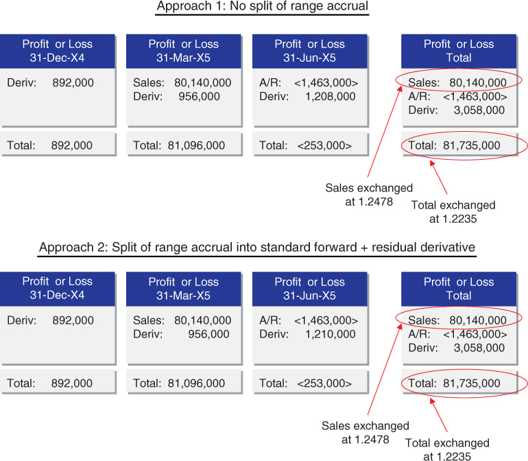
Figure 5.40 Comparison of effects in profit or loss.
Two approaches were analysed: a first approach designating the whole range accrual as the hedging instrument, and a second approach splitting the range accrual into a standard forward and a residual derivative. Whilst both approaches resulted in an identical profit or loss structure, as shown in Figure 5.40, this outcome is not to be generalised because it is largely dependent on the behaviour of the EUR–USD spot rate during the life of the hedge.
ABC expected 70% of the EUR–USD fixings to fall within the accrual range. A large deviation from this percentage meant that ABC could be either overhedged or underhedged, adding undesired exposure to the EUR–USD rate. In our case, ABC was fortunate because while it ended up being overhedged, it unwound the excess hedge at favourable market rates. From an economic perspective, the range accrual performed very well. The USD 100 million sale proceeds were exchanged for EUR 81,735,000, implying a 1.2235 exchange rate, notably better than the 1.2500 original forward rate.
5.17 HEDGING ON A GROUP BASIS – THE TREASURY CENTRE CHALLENGE
Hedging activity using treasury centres may face particular accounting issues under IFRS 9, especially when internal hedges are involved. This section analyses the accounting implications when using a treasury centre to manage a whole group's foreign exchange risk.
It is a well-established practice in most large companies to centralise financial hedging activities into a group treasury centre. Treasury centres manage a broad range of functions for the group, including global cash and liquidity management, bank relationship management, funding of debt and equity, and risk management. Some companies have a single treasury centre that is based at corporate headquarters or a tax-efficient location, while others establish several centres, each strategically located to meet the needs of a specific region.
When hedging financial risk, the treasury centre of a group serves as an in-house bank netting off exposures arising across the group. Exposures are identified at the subsidiary level, and these subsidiaries then hedge using internal deals with the centre. The treasury centre then lays off the net risk position with external parties. This hedging approach is more efficient than having each subsidiary independently working with banks to hedge their local financial risk.
The following case study sheds some light on the accounting challenges faced by a centralised hedging policy. Suppose that a consolidated group has the structure shown in Figure 5.41. The group, whose presentation currency is the EUR, comprises a parent company, a treasury centre and three subsidiaries, A, B and C, whose functional currencies are the EUR, USD and JPY, respectively.
Figure 5.41 Group entities.
Subsidiary A's revenues were in EUR, GBP and JPY. It forecasted revenues of EUR 60, GBP 30 (i.e., the equivalent in GBP to EUR 30) and JPY 30. It forecasted sales costs related to those revenues of EUR 70 and JPY 30. For the sake of simplicity, suppose that all the flows were expected to take place on the same date. To hedge its exposure to GBP risk, Subsidiary A entered into an FX forward with the treasury centre at market rates, in which Subsidiary A agreed to sell GBP 30 and to buy EUR 30 on the date that the cash flows were expected to take place.
Subsidiary B's revenues were in USD, EUR and JPY. It forecasted revenues of USD 70 (i.e., the equivalent in USD to EUR 70), EUR 30 and JPY 30. It forecasted sales costs related to those revenues of USD 70 and JPY 30. For the sake of simplicity, suppose that all the flows were expected to take place on the same date. To hedge its exposure to EUR risk, Subsidiary B entered into an FX forward with the treasury centre at market rates, in which Subsidiary B agreed to sell EUR 30 and to buy USD 30 on the date that the cash flows were expected to take place.
Subsidiary C's revenues were in JPY and USD. It forecasted revenues of JPY 70 (i.e., the equivalent in JPY to EUR 70) and USD 30. It forecasted sales costs related to those revenues of JPY 70. For the sake of simplicity, suppose that all the flows were expected to take place on the same date. To hedge its exposure to USD risk, Subsidiary C entered into an FX forward with the treasury centre at market rates, under which Subsidiary C agreed to sell USD 30 and to buy JPY 30 on the date that the cash flows were expected to take place.
As a result, the treasury centre's net exposure with the subsidiaries was a long GBP 30 and a short JPY 30 (see Figure 5.42). In order to hedge that net exposure, the treasury centre entered into an FX forward with an external bank under which it agreed to sell GBP 30 and to buy JPY 30.
| EUR | GBP | JPY | USD | |
| Subsidiary A | – 30 | + 30 | + 30 – 30 | |
| Subsidiary B | + 30 | + 30 – 30 | – 30 | |
| Subsidiary C | - 30 | + 30 | ||
| Total | -0- | + 30 | - 30 | -0- |

Figure 5.42 Group FX hedges.
5.17.1 Accounting Implications at Subsidiary Level
At a subsidiary level the hedges posed no particular accounting issues when preparing their entity-only financial statements. For example, in the case of Subsidiary A (see Figure 5.43), it could apply hedge accounting, assuming all other requirements were met, as the counterparty to the forward (the treasury centre) was an entity external to Subsidiary A and as the forecast transaction was highly probable and would be affecting profit or loss. Subsidiary A would designate the EUR–GBP forward as the hedging instrument in a cash flow hedge of its foreign currency denominated highly probable revenues of GBP 30 (the hedged item). Effective amounts of the changes in the fair value of the FX forward would be recorded in the cash flow hedge reserve of equity and reclassified to profit or loss when the hedged revenues ultimately affected profit or loss.
Figure 5.43 Subsidiary A's hedging position.
Whilst hedge accounting could not be applied (a derivative in itself cannot be a hedged item), from an accounting perspective the three internal hedges in conjunction with the external hedge did not pose a major challenge to the treasury centre. It measured all the FX forwards at fair value with changes in fair value recorded in profit or loss. As all the changes in these fair values were largely offset, the treasury centre had no volatility in profit or loss other than that caused by the CVAs/DVAs to the fair valuations of the forwards.
5.17.2 Accounting Implications at Consolidated Level
A key requirement of hedge accounting under IFRS 9 is that all hedging derivatives must involve a counterparty external to the entity (or group entities) being accounted for. Intragroup derivatives are not eligible for hedge accounting treatment in the consolidated accounts, causing significant difficulties where a group operates through a treasury centre. In these circumstances and in order to achieve hedge accounting it is usually necessary to identify, on a one-to-one basis, exposures in the group with external parties that may be designated as hedged items. In other words, the treasury centre would need to identify sufficient exposures in each of its various subsidiaries and designate, on a potentially arbitrary basis, some of those exposures on a one-to-one basis with its external contract.
Need to Split the JPY–GBP Forward?
The JPY–GBP forward hedged two separate risks: (i) a JPY–EUR exchange rate risk and (ii) a EUR–GBP exchange rate risk. The first the parent company needed to assess was whether it needed to split the JPY–GBP forward into two separate instruments: a JPY–EUR forward (selling EUR and buying JPY) and a EUR–GBP forward (selling GBP and buying EUR), as shown in Figure 5.44. This split, if needed, would undermine one of the main advantages of treasury centres: to lower the transaction costs of hedging.

Figure 5.44 Treasury Centre's hedging position.
Fortunately, IFRS 9 allows a single hedging instrument to be designated as a hedging instrument for more than one type of risk, provided that there is a specific designation of the hedging instrument and of the different risk positions as hedged items. In our case there was no need to split the external hedge into two separated contracts, or in other words, the single forward contract could be designated as hedging instrument in two separate hedging relationships:
- In a first hedging relationship, the risk being hedged was clearly identified as the exposure to variations in the JPY–EUR exchange rate. The hedged item was the cash flow stemming from highly expected purchases denominated in JPY, whose fair value could be reliably measured. The hedging instrument was the JPY receipt on the forward contract, whose fair value could be reliably measured.
- In a second hedging relationship, the risk being hedged was clearly identified as the exposure to variations in the EUR–GBP exchange rate. The hedged item was the cash flow stemming from highly expected sales denominated in GBP, whose fair value could be reliably measured. The hedging instrument was the GBP payment on the forward contract, whose fair value could be reliably measured.
JPY Risk: Hedge Item Candidate 1 Eligibility
The group could apply hedge accounting on consolidation in a cash flow hedging relationship in which the JPY leg of the JPY–GBP forward taken out by the treasury centre would be the hedging instrument and the cash flow stemming from Subsidiary A's highly expected forecast JPY purchase would be the hedged item, as shown in Figure 5.45, assuming all other requirements for hedge accounting were met.

Figure 5.45 Hedge item candidates for the JPY exposure.
This qualification was due to the direct future incorporation of Subsidiary A's JPY purchase in consolidated profit or loss, being converted into the group's EUR presentation currency. The exposure to movements in the JPY–EUR exchange rate constituted a cash flow risk, and therefore could be subject to cash flow hedge accounting.
JPY Risk: Hedge Item Candidate 2 Eligibility
The group could not apply hedge accounting on consolidation in a cash flow hedging relationship in which the JPY leg of the JPY–GBP forward taken out by the treasury centre would be the hedging instrument and the cash flow stemming from Subsidiary B's highly expected forecast JPY purchase would be the hedged item, as shown in Figure 5.45.
This non-qualification occurred because there was no JPY–EUR cash flow exposure that could affect consolidated profit or loss. Whilst Subsidiary B was exposed to movements in the JPY–USD exchange rate and Subsidiary B's USD profit or loss was translated into EUR upon consolidation (see Chapter 6), the exposure of the group to the JPY was an indirect exposure, constituting a translation risk rather than a cash flow exposure.
JPY Risk: Hedge Item Candidate 3 Eligibility
The group could not apply hedge accounting on consolidation in a cash flow hedging relationship in which the JPY leg of the JPY–GBP forward taken out by the treasury centre would be the hedging instrument and the cash flow stemming from Subsidiary C's highly expected forecast JPY purchase would be the hedged item, as shown in Figure 5.45.
This non-qualification occurred because there was no JPY–EUR cash flow exposure that could affect consolidated profit or loss. Subsidiary C was not exposed to movements in the JPY as its functional currency was the JPY. Whilst Subsidiary C's JPY profit or loss was translated into EUR upon consolidation, the exposure of the group to the JPY was an indirect exposure, constituting a translation risk rather than a cash flow exposure.
However, Subsidiary C's JPY profit or loss would become part of the net investment of the group in Subsidiary C, and consequently, changes in the JPY–EUR exchange rate would affect the cumulative translation adjustment upon consolidation (see Chapter 6). As a result, the group could apply net investment hedge accounting in a hedging relationship in which the hedging instrument would be the JPY leg of the JPY–GBP forward taken out by the treasury centre and the hedged item would be the JPY-denominated net assets of Subsidiary C.
Conclusions
When a treasury centre is involved, the application of hedge accounting on the consolidated statements requires a process of arbitrary designation of the hedged item. At first sight it looks as if this process only involves an additional administrative burden. In reality the designation process is much more complicated than in our example.
First of all, bear in mind that the above example was much simplified as all the expected cash flows were expected to take place on the same date. In reality, there is often a time lag between timing of the external hedges and the timing of the identified hedged items. Timing differences may create significant hedge ineffectiveness.
Secondly, it was assumed that the treasury centre netted out the group's exposure under the internal derivatives and the external derivatives. In reality, a treasury centre may decide to keep some residual risk or to hedge using a different currency pair, complicating matters further. For example, a foreign exchange exposure may be created by an illiquid currency and a treasury centre may prefer to take out a hedge on a different currency that is highly correlated to the illiquid one.
5.18 HEDGING FORECAST INTRAGROUP TRANSACTIONS
In its consolidated financial statements, a group may designate as the hedged item in a foreign currency cash flow hedge, a highly probable forecast transaction with an external party to the group, provided that the transaction is denominated in a currency other than the group's functional currency.
Whilst in general IFRS 9 does not permit an intragroup item to be a hedged item in the consolidated financial statements, there is an exception to this general rule:
- When the intragroup monetary item results in an exposure to foreign exchange rate gains or losses that are not fully eliminated on consolidation in accordance with IAS 21 The Effects of Changes in Foreign Exchange Rates. In accordance with IAS 21, foreign exchange rate gains and losses on intragroup monetary items are not fully eliminated on consolidation when the intragroup monetary item is transacted between two group entities that have different functional currencies.
- In the case of a highly probable forecast intragroup transaction, the transaction is denominated in a currency other than the functional currency of the entity entering into that transaction and the foreign currency risk will affect consolidated profit or loss.
The following are examples of forecast intragroup transactions that could result in the foreign exchange risk affecting consolidated profit or loss:
- Forecast sales and purchases of inventories between entities in a group with a subsequent sale of the inventory to a party external to the group. Any hedging gains or losses that are initially recognised in equity are reclassified to profit or loss in the same period that the foreign currency risk affects consolidated profit or loss. This would occur when the onward sale to the external party occurs (and not when intragroup sales occurs) because that is when the hedged transaction affects consolidated profit or loss.
- A forecast intragroup sale of equipment from a group entity that manufactured it to another group entity that uses the equipment. When the purchasing entity depreciates the equipment, the amount initially recognised in the consolidated financial statements for the equipment may change because the transaction is denominated in a currency other than the functional currency of the purchasing entity. In this example, a related external transaction does not exist and the item affects consolidated profit or loss.
Examples of forecast intragroup transactions unlikely to result in the foreign exchange risk affecting consolidated P&L are intragroup management fees, interest on intragroup loans or intragroup royalty payments.
IFRS 9 does not explicitly consider situations where the intragroup transaction is committed rather than forecast. In my view, committed transactions are also eligible for hedge accounting since they have a higher probability of occurrence.
5.18.1 Example of Hedge of Forecast Intragroup Transaction
ABC is a group that comprises operating subsidiaries A and B. The group has the EUR as its functional currency. Subsidiary A's functional currency is the GBP while Subsidiary B's functional currency is the USD.
Subsidiary A incurs most of its production costs in EUR. It sells most of its production to Subsidiary B, and these transactions are denominated in USD. In turn, Subsidiary B sells the product on to external customers, also in USD. Subsidiary A forecasts in March 20X6 that it will sell in June 20X6 USD 100 million of inventory to Subsidiary B. These sales are highly probable, and all the other IFRS 9 conditions for hedge accounting are met. Subsidiary B expects to sell this inventory to external customers in early September 20X6.
In January 20X6 Subsidiary A enters into a EUR–USD derivative to hedge its expected sale of USD 100 million to Subsidiary B in June 20X6.
The USD 100 million forecast intragroup sales can be designated in the consolidated financial statements as a hedged item in a foreign currency cash flow hedge (see Figure 5.46) as:
- the sales are highly probable, and all other conditions for using hedge accounting are met;
- the hedge is a cash flow hedge of foreign currency risk;
- the sales are denominated in a currency (USD) other than Subsidiary A's functional currency (EUR); and
- the existence of the expected onward sale of the inventory to third parties results in the hedged exposure affecting consolidated profit or loss.

Figure 5.46 Hedging relationship.
Gains and losses on the EUR–USD derivative would be recognised in consolidated equity, to the extent that the hedge is effective. These amounts would be reclassified to consolidated profit or loss in September 20X6 when the external sales occur (i.e., when the hedged transaction affects consolidated profit or loss).