
Chapter 8. Table Design
Accumulo provides application developers with a high degree of control over data layout, which has a large effect on the performance of various access patterns. Here we discuss some table designs for various purposes and address particular issues in designing keys, values, and authorizations.
Single-Table Designs
Some applications require looking up values based on a few specific pieces of data most of the time. In these cases it is convenient to identify any hierarchies that may exist in the data and to build a single table that orders the data according to the hierarchy.
For example, if we are writing an application to store messages, such as email, we might have a hierarchy that consists of user accounts identified by unique email addresses. Within a user account we have folders, and each folder contains zero or more email messages (Figure 8-1).
In addition to natural hierarchies in the data, we also need to consider access patterns. A common query will be to access a list of messages to or from a user within a particular folder, preferably in time order from most recent to oldest.
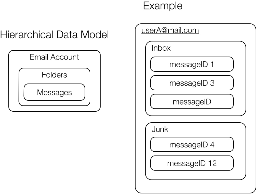
Figure 8-1. Hierarchy in data
An example application method for fetching this data can look like the following:
listMessages(emailAddress, folder, offset, num)
where emailAddress is the user’s email address, folder indicates which mail folder to access, and offset and num together indicate which set of messages to fetch for the purposes of displaying email addresses in pages.
The first page would have an offset of 0 and could have a num of 100 to show the first (most recent) 100 email messages.
To support reading this data efficiently, we could store all the messages that belong to a user under a row ID consisting of the user’s email address, followed by the folder, and finally, the date and time at which the email was created or arrived. We may also want to store a unique identifier for this email at the end, to distinguish messages that arrive at the same time. Our row IDs then would look something like this:
[email protected]_inbox_20110103051745_AFBBE
where [email protected] is the email address, followed by the folder name (inbox), followed by a zero-padded date and time representation that is designed to sort dates properly, followed by a hash of some part of the email or perhaps an ID that is delivered in the email header.
This works, except that using the human-readable representation of the data would order our keys in ascending time order, rather than descending as most email applications do. To change this, we can transform the representation of the date in the row ID so that they sort in reverse time order. One way to do this is to subtract the date from a number larger than the largest date we expect to ever store. For example, the date element could be subtracted from the number 99999999999999. We could store the actual date in a value in this row.
Note that we’re using an underscore as the delimiter here. A different delimiter may be required depending on whether we ever need to parse the row ID and whether underscores are valid characters for the elements of the row ID.
We then need to determine how to store each part of the message. We can decide to break out the subject and body into different columns so that users can quickly get a list of messages showing the subject without having to read all of the bodies of those messages. Other times, a user will need to retrieve an entire message, including the body and subject. The application method to retrieve all the data for a single message can look like the following:
getMessage(emailAddress, folder, date, emailId)
So we can have one column family for small amounts of data like the subject, and another column family for the email bodies. This will allow us to store those two column families in different locality groups, which means we can efficiently read one from disk without reading the other, and other times we can still read them both fairly efficiently.
Now a message in our table may look like Table 8-1.
| Row | Column family | Column qualifier | Value |
|---|---|---|---|
|
|
|
|
|
|
|
|
|
|
|
This one table can now fulfill both types of requests.
The implementation of listMessages() without paging would involve creating a single scan such as:
publicIterator<Entry<Key,Value>>listMessages(StringemailAddress,Stringfolder,Authorizationsauths){Scannerscanner=inst.createScanner("emailMessagesTable",auths);// we only want to scan over the 'details' column familyscanner.fetchColumnFamily("details");scanner.setRange(Range.prefix(emailAddress+"_"+folder));returnscanner.iterator();}
Similarly, the implementation of getMessage() would involve creating a single scan such as:
publicIterator<Entry<Key,Value>>listMessages(StringemailAddress,Stringfolder,Stringdate,StringemailID,Authorizationsauths){StringtransformedDate=(99999999999999-Integer.parseInt(date)).toString();Scannerscanner=inst.createScanner("emailMessagesTable",auths);// we want all column families, and so we don't fetch a particular familyscanner.setRange(Range.exact(emailAddress+"_"+folder+"_"+transformedDate+"_"+emailID));returnscanner.iterator();}
In this example, our table exploits natural hierarchies in the data and addresses the two most common access patterns for retrieving information for an application. There are any number of variations on this theme, but a design involving a single table is limited in the number of ways the data can be accessed. For example, this table would not support finding email messages that contain one or more search terms. For those access patterns, additional tables for secondary indexes are necessary.
Implementing Paging
By default, scanners return key-value pairs until the set of results is exhausted. Applications that want to enable users to page through results have several options.
For example, we can create a method that takes a start row ID, a set of columns, a page offset, and a page size:
publicList<Entry<Key,Value>>getResults(StringstartRow,List<Text>columns,intoffset,intpageSize)
We can choose to create brand-new Scanner objects every time this method is called, and skip over the previous page until we reach the specified offset.
This has the disadvantage of having to read more and more results off of disk and transfer them to the client as the page offset increases.
If users will typically only look at the first few pages this might be acceptable.
An example of using Google’s Guava library to modify a Java iterator returned from a Scanner is as follows:
importcom.google.common.collect.FluentIterable;publicList<Entry<Key,Value>>getResults(StringstartRow,List<Text>columns,intoffset,intpageSize){// ... after the scanner has been setupFluentIterable<Entry<Key,Value>>fiter=FluentIterable.from(scanner);fiter.skip(offset);fiter.limit(pageSize);returnLists.newArrayList(fiter);}
Another option is to cache recently created scanners and associate them with individual queries. When users request the next page in a set of results, we can simply retrieve the scanner and continue fetching the next page of key-value pairs. Scanners do not have the ability to seek backward, but if the primary method of paging through results is to start at the first and move through the pages sequentially, this method may work well. This has the disadvantage of having to keep scanners around and expire them after a certain amount of time or until the user closes the session.
Another option for paging forward is to, instead of caching Scanner objects, cache the last key-value pair seen and then create a new scanner, seeking to the next logical key that appears after the last key-value pair seen.
This has the advantage of not requiring scanner resources to be kept open, but it can incur more overhead by creating a new scanner for every page requested.
When paging is implemented in the context of secondary indexes, we need to process record IDs retrieved from the index table that match the query criteria to identify the page of records requested, and then fetch only matching actual records for that page.
Secondary Indexing
Applications that use a single table and employ a simple access pattern are among the most scalable, consistent, and fast. This type of design can serve in a wide variety of applications. When storing records in an Accumulo table, we can store them in sorted order but can only sort them one way.
In the previous example we stored emails in order of the recipient’s email address, then by the date, and finally by a unique email ID. In this case the record ID used is a concatenation of those three elements. If we want to look up records based on other criteria, we have to scan the entire table. For these other access patterns, building a secondary index can provide a solution. These applications still need to minimize the work done at query time, to ensure high performance as the amount of data and the number of concurrent users increase.
Secondary indexes are tables that allow users to quickly identify the record IDs that contain a value from a particular field. Those record IDs can then be used to retrieve the full record from the primary table containing records. We’ll next discuss two types of secondary indexes: a term-partitioned index and a document-partitioned index.
Index Partitioned by Term
One way to build a secondary index is by storing individual terms to be queried in the row ID. For example, we can retrieve Wikipedia pages that contain a given word by building a table storing the words found in article text in the Accumulo row ID and the article title as the column qualifier.
Table 8-2 recalls our WikipediaArticles table from “Data Modeling”, which used article titles as the row ID.
| Row | Column family | Column qualifier | Column visibility | Value |
|---|---|---|---|---|
page title |
contents |
contents visibility |
page contents |
|
page title |
metadata |
id |
id visibility |
id |
page title |
metadata |
namespace |
namespace visibility |
namespace |
page title |
metadata |
revision |
revision visibility |
revision |
page title |
metadata |
timestamp |
timestamp visibility |
timestamp |
Now we create a secondary index that maps words appearing in Wikipedia pages to the page titles, shown in Table 8-3. An index organized by storing words or terms as the row ID is referred to as a term-partitioned index.
| Row | Column family | Column qualifier | Column visibility | Value |
|---|---|---|---|---|
word |
contents |
page title |
page visibility |
The entries for an index on a subset of Wikipedia articles are as follows:
white contents:Friendship_Games []
white contents:Olympic_Games []
white contents:Olympic_Games_ceremony []
whitfield, contents:Cotswold_Olimpick_Games []
whitsun, contents:Cotswold_Olimpick_Games []
whitsun. contents:Cotswold_Olimpick_Games []
who contents:Alternate_Olympics []
who contents:Ancient_Olympic_Games []
who contents:Arena_X-Glide []
Because in a secondary index table we’re swapping the order of the row IDs and values from the original table, an index like this is sometimes called an inverted index. However, note that we don’t store the title from the WikipediaArticles table in the value portion of the secondary index, but rather we store titles in the column qualifier. This is because a term can appear in more than one article. We don’t want article titles to be different versions of values for the terms, and we could envision wanting to scan a range of titles within a term, so we simply store the titles under the column qualifier and leave the value blank.
This technique also works for indexing the article metadata fields. It is possible to store the index entries for all fields in the same table if we want (see Table 8-4). We’ll store the concatenated column family and qualifier from the original table in the column family of the index so that a client can fetch values from a particular column, if they so choose. By not specifying the column family, a client can find the rows in which a given value appears in any field.
| Row | Column family | Column qualifier | Column visibility | Value |
|---|---|---|---|---|
word |
contents |
page title |
page visibility |
|
id |
metadata:id |
page title |
page visibility |
|
namespace |
metadata:namespace |
page title |
page visibility |
|
revision |
metadata:revision |
page title |
page visibility |
|
timestamp |
metadata:timestamp |
page title |
page visibility |
Note
When we build a secondary index table, one value from the original table can become many key-value pairs if we are tokenizing the text of the original values and storing a key-value pair for every individual word in the index. Index tables are a good example of using up more disk space to gain speed when doing searches.
In this case, we’re using roughly twice the disk space of our original table in order to avoid doing expensive table scans. Developers of relational databases will recognize this trade-off, because relational database indexes are also stored on disk. Accumulo’s default compression techniques can help mitigate the additional disk space used.
Not only does this require additional disk space, but it will also take longer to write this data from clients because we’re now writing not only the original record, but also some number of index entries. Application designers should consider the impact on ingest speed versus the speed up gained for queries and choose which fields, if any, to write to a secondary index based on the types of queries required.
The horizontal scalability of Accumulo’s design makes accommodating additional precomputation such as this a matter of simply adding more hardware resources.
An example of an ingest client that writes data to the WikipediaArticles table and the WikipediaIndex table at the same time is as follows:
// write article data to articles table as beforeStringwikitext=page.getText();Stringplaintext=model.render(converter,wikitext);plaintext=plaintext.replace("{{"," ").replace("}}"," ");Mutationm=newMutation(page.getTitle());m.put(WikipediaConstants.CONTENTS_FAMILY,"",plaintext);m.put(WikipediaConstants.METADATA_FAMILY,WikipediaConstants.NAMESPACE_QUAL,page.getNamespace());m.put(WikipediaConstants.METADATA_FAMILY,WikipediaConstants.TIMESTAMP_QUAL,page.getTimeStamp());m.put(WikipediaConstants.METADATA_FAMILY,WikipediaConstants.ID_QUAL,page.getId());m.put(WikipediaConstants.METADATA_FAMILY,WikipediaConstants.REVISION_QUAL,page.getRevisionId());writer.addMutation(m);// write index entries as well// tokenize article contents on whitespace and punctuation and set to lowercaseHashSet<String>tokens=Sets.newHashSet(plaintext.replace(""","").toLowerCase().split("\s+"));for(Stringtoken:tokens){if(token.length()<2){// skip single letterscontinue;}MutationindexMutation=newMutation(token);indexMutation.put(WikipediaConstants.CONTENTS_FAMILY,page.getTitle(),BLANK_VALUE);indexWriter.addMutation(indexMutation);}

Create a new
Mutationwith the term that users can query as the row ID.
Designate this index entry as being from the article contents by specifying a column family. Store the page title in the column qualifier so that we use it to perform a subsequent lookup on the primary articles table.
We’re only indexing simple words here, by tokenizing the original text on whitespace. We talk about how to index other types of values in “Indexing Data Types”.
Now we have a table containing original articles, with the article title as the key, and another table containing index entries of words found in articles with pointers to the article titles from which they came.
Querying a Term-Partitioned Index
With this term-partitioned secondary index we can now look up article titles by the value of any metadata field, or by any word appearing in the article body.
Once we have some article titles retrieved from the index table, we can retrieve the information about the articles by doing lookups against the original WikipediaArticles table using a BatchScanner:
publicvoidquerySingleTerm(Stringterm)throwsTableNotFoundException{Scannerscanner=conn.createScanner(WikipediaConstants.INDEX_TABLE,auths);// lookup term in indexscanner.setRange(Range.exact(term));// store all article titles returnedHashSet<Range>matches=newHashSet<>();for(Entry<Key,Value>entry:scanner){matches.add(newRange(entry.getKey().getColumnQualifier().toString()));}if(matches.isEmpty()){System.out.println("no results");return;}for(Entry<Key,Value>entry:retrieveRecords(conn,matches)){System.out.println("Title: "+entry.getKey().getRow().toString()+" Revision: "+entry.getValue().toString()+" ");}}privateIterable<Entry<Key,Value>>retrieveRecords(Connectorconn,Collection<Range>matches)throwsTableNotFoundException{// retrieve original articlesBatchScannerbscanner=conn.createBatchScanner(WikipediaConstants.ARTICLES_TABLE,auths,10);bscanner.setRanges(matches);// fetch only the article contentsbscanner.fetchColumn(newText(WikipediaConstants.METADATA_FAMILY),newText(WikipediaConstants.REVISION_QUAL));returnbscanner;}
Note that our query code is coupled with our ingest code. If we change our ingest code, the schema of our index or original articles table will change and our query code will have to be updated in order to query these tables properly.
The query we just performed is an example of a point query, in which we find all records containing an exact term. We can also use this index to perform range queries, in which we retrieve all records matching a range of terms. See “Using Lexicoders in indexing” for an example.
Dealing with the nuances of secondary indexing in applications will be new to developers accustomed to working with relational databases, which do the work of building secondary indexes for applications. The trade-off for having to do this work is an incredible amount of flexibility in how data is indexed and retrieved.
This level of control is appropriate for Accumulo because the large data volumes Accumulo is designed to manage make it imperative for data to be organized in ways that are optimized for specific access patterns; otherwise performance will quickly degrade.
A suboptimal query on even a few gigabytes of data, such as a simple linear scan, can still be done quickly because that much data will fit comfortably in the main memory a single server and even a single desktop or notebook computer. But sub-optimal queries on hundreds of terabytes of data will be too slow for users to tolerate.
One way to view indexing is as a way to precompute views of the data that are optimal for the required access patterns. The scalability of the system and the relatively low cost of storage makes materializing these views feasible.
Combining query terms
In the previous example we were only querying for a single term or a single range of terms at a time. If we needed to look up records that satisfy more than one criterion—say, for example, all Wikipedia articles containing the word baseball with a timestamp newer than a year ago—we would need to do separate scans for each criterion and combine the article titles returned to get articles that match both criteria. To be specific, each scanner returns a set of titles matching the scan criterion applied, and the intersection of those sets of titles represents articles that match all criteria. The union of those sets of titles would represent articles that match at least one criterion.
A simple implementation that uses one HashSet to determine records that match any term is as follows:
// returns records matching any termpublicvoidqueryMultipleTerms(String...terms)throwsTableNotFoundException{HashSet<String>matchingRecordIDs=newHashSet<>();for(Stringterm:terms){Scannerscanner=conn.createScanner(WikipediaConstants.INDEX_TABLE,auths);// lookup term in indexscanner.setRange(Range.exact(term));for(Entry<Key,Value>entry:scanner){matchingRecordIDs.add(entry.getKey().getColumnQualifier().toString());}}if(matchingRecordIDs.isEmpty()){System.out.println("no results");return;}// convert to RangesList<Range>ranges=Lists.newArrayList(Iterables.transform(matchingRecordIDs,newStringToRange()));for(Entry<Key,Value>entry:retrieveRecords(conn,ranges)){System.out.println("Title: "+entry.getKey().getRow().toString()+" Revision: "+entry.getValue().toString()+" ");}}privateclassStringToRangeimplementsFunction<String,Range>{@OverridepublicRangeapply(Stringf){returnnewRange(f);}}
For multiple single-term lookups—such as all articles that contain both the word baseball and record—we can take advantage of the fact that the article titles, which are stored in the column qualifier, are sorted within a single row and column family. We can combine the titles returned from two single-term scans by simply comparing the titles as they are returned from each scan to find matches, rather than having to load all the titles in memory and perform set intersection using something like Java collections. This is important because we often can’t predict how many records will match a given criterion.
Problems can arise when queries become more complex than this. Some of these can be better addressed via a document-partitioned index, as described in “Index Partitioned by Document”.
Querying for a term in a specific field
In our previous example, we were looking for index entries that match our query term, regardless of the field in which our term may have appeared in the original record. We can execute a more focused query by specifying a field in which our term must appear, presuming we’ve stored this field information in the key of our index.
For example, if we want only articles in which the term wrestling appears in the body of the article, we can limit the range of our initial scanner to entries representing an appearance of the word wrestling within the body of the article.
When we created our index, we used the column family to store information about the field from which an index term originated.
So we can simply construct a range covering the exact row and column we want when configuring our scanner.
When scanning only one row, this is more efficient than using the fetchColumn() method, because no key-value pairs in other columns will be iterated over and rejected.
Modifying our query from the previous example, we have:
Scannerscanner=conn.createScanner(WikipediaConstants.INDEX_TABLE,auths);// lookup term and field in indexscanner.setRange(Range.exact(term),WikipediaConstants.CONTENTS_FAMILY);// store all article titles returnedHashSet<Range>matches=newHashSet<>();for(Entry<Key,Value>entry:scanner){matches.add(newRange(entry.getKey().getColumnQualifier().toString()));}if(matches.isEmpty()){System.out.println("no results");return;}for(Entry<Key,Value>entry:retrieveRecords(conn,matches)){System.out.println("Title: "+entry.getKey().getRow().toString()+" Revision: "+entry.getValue().toString()+" ");}
Now we include the column family in range, which identifies the field in which the search term appears.
It is even possible to build an index across tables this way, by storing the table name in the key. For example, we could choose to build our index to store information as in Table 8-5.
| Row | Column family | Column qualifier | Column visibility | Value |
|---|---|---|---|---|
value |
originalTable-field |
record ID |
page visibility |
This type of index would allow queries to be performed across multiple data sets simultaneously. The flexibility of index tables allows for options such as this.
Maintaining Consistency Across Tables
Term-based secondary indexes must be maintained along with the original table so that inconsistencies do not arise. Even though Accumulo does not provide multirow transactions or cross-table transactions, this consistency can often be managed in the application.
One strategy for managing consistency between the original table and the secondary index table is to carefully order read and write operations. You can choose to wait until new rows are written to the original table first, and then write the corresponding entries to the secondary index. If for some reason a write to the original table fails, it can be retried before any index entries are written. This way clients aren’t referred by the index to a row in the original table that doesn’t exist.
Inversely, when data is deleted from the original table, the index entries should be removed first, and then the row from the original table. These strategies will prevent any clients from looking up data in the index that has not yet been written or that has been removed from the original table.
More complicated strategies may be required if an application involves concurrent updates to indexed data. One potential way to address updating secondary indexes is to look to higher-level abstractions built on top of Accumulo, such as the Fluo framework, which allows writes to be triggered to index tables from updates to a primary record table.
Using MultiTableBatchWriter for consistency
We introduce the MultiTableBatchWriter in “Writing to Multiple Tables”.
The MultiTableBatchWriter has close() and flush() methods that allow applications to push new data to multiple tables and verify that they were written successfully.
This can help when synchronizing writes to secondary indexes while writing to original tables.
To use a MultiTableBatchWriter in our indexing example, we’ll first create a MultiTableBatchWriter and use it to obtain the individual BatchWriter objects for our index and record table:
BatchWriterConfigconf=newBatchWriterConfig();MultiTableBatchWritermultiTableBatchWriter=conn.createMultiTableBatchWriter(conf);writer=multiTableBatchWriter.getBatchWriter(WikipediaConstants.ARTICLES_TABLE);indexWriter=multiTableBatchWriter.getBatchWriter(WikipediaConstants.INDEX_TABLE);
Our application can keep track of mutations and call flush() periodically to determine when a batch has been written successfully or that a set of mutations should be retried.
Instead of calling flush() on individual BatchWriter objects, we instead call it on our MultiTableBatchWriter like this:
try{multiTableBatchWriter.flush();}catch(MutationsRejectedExceptionmre){// report or retry}
Also, when we are done writing data, we call close() on our MultiTableBatchWriter instead of individual BatchWriters:
try{multiTableBatchWriter.close();System.out.println("done.");}catch(MutationsRejectedExceptionmre){// report or retry}
See the full listing of WikipediaIngestMultiTableExample.java for details.
Index Partitioned by Document
A basic term-partitioned index is useful for retrieving all the data containing a particular word or having a specific value for a field. If we need to find all the data containing two different words, the client code would have to issue two scans to the basic index, bringing the document IDs for both back to the client side and intersecting the two lists. This can be inefficient if one or both of the terms appears in many documents, requiring many IDs to be retrieved. One solution to this problem is to build a document-partitioned index. In such an index, sets of documents are grouped together into partitions, and each partition is assigned an ID. The index is organized first by partition ID, then by word. Table 8-6 shows an example.
| Row | Column family | Column qualifier | Column visibility | Value |
|---|---|---|---|---|
partition ID |
doc � wikiDoc |
page title |
page visibility |
page contents |
partition ID |
ind |
word � wikiDoc � page title � info |
page visibility |
The partition ID is the row portion of the key.
The page contents are stored in one column family of the row, and the index is stored in another column family.
To retrieve all the pages containing the words “wrestling” and “medal” in this partition, we can read over and merge the sorted lists of page titles obtained by scanning over the keys starting with partition ID_ : index : wrestling and starting with partition ID : index : medal.
This intersection can be accomplished on the server side with an appropriate Accumulo iterator. We discuss iterators in more depth in “Iterators”. An iterator that seeks to multiple starting points and intersects the results is called an intersecting iterator.
To use this method, a data set should be divided into an appropriate number of partitions so that the partitions are not too large or too small, and there are enough of them that they are spread over the desired number of servers. Ideally each partition will fill an entire tablet, so its size should be somewhere between 256 MB and tens of gigabytes. For the Wikipedia data, we’ll use 32 partitions.
Example code for building this table is as follows:
privatestaticfinalintNUM_PARTITIONS=10;privatestaticfinalValueBLANK_VALUE=newValue("".getBytes());@Overridepublicvoidprocess(WikiArticlearticle,Siteinfoinfo)throwsSAXException{Stringwikitext=article.getText();Stringplaintext=model.render(converter,wikitext);plaintext=plaintext.replace("{{"," ").replace("}}"," ");Mutationm=newMutation(Integer.toString(Math.abs(article.getTitle().hashCode())%NUM_PARTITIONS));m.put("doc"+'�'+"wikiDoc",article.getTitle(),plaintext);// tokenize article contents on whitespace and punctuation and set to lowercaseHashSet<String>tokens=Sets.newHashSet(plaintext.toLowerCase().split("\s+"));for(Stringtoken:tokens){m.put("ind",token+'�'+"wikiDoc"+'�'+article.getTitle()+'�',BLANK_VALUE);}try{writer.addMutation(m);}catch(MutationsRejectedExceptione){thrownewSAXException(e);}}
Tip
Unlike term-partitioned indexes, in a document-partitioned table Accumulo can make all the inserts for a given document atomically because they are all inserted into the same row. The trade-off is that all partitions must be searched when performing queries.
Key-value pairs in this table look as follows:
root@miniInstance> table WikipediaPartitioned
table WikipediaPartitioned
root@miniInstance WikipediaPartitioned> scan
scan
0 docx00wikiDoc:Sqoop []     Infobox software Sqoop is a ...
0 ind:x00wikiDocx00Sqoopx00 []
0 ind:2012.x00wikiDocx00Sqoopx00 []
0 ind:ax00wikiDocx00Sqoopx00 []
0 ind:accumulox00wikiDocx00Sqoopx00 []
0 ind:alsox00wikiDocx00Sqoopx00 []
0 ind:andx00wikiDocx00Sqoopx00 []
0 ind:apachex00wikiDocx00Sqoopx00 []
0 ind:applicationx00wikiDocx00Sqoopx00 []
0 ind:archivesx00wikiDocx00Sqoopx00 []
Querying a Document-Partitioned Index
When querying the data, we will use a BatchScanner along with an intersecting iterator, the IndexedDocIterator, to find relevant pages in each of the partitions.
To scan all partitions, we give the BatchScanner a special range that covers the entire table.
Code to query our document-partitioned index is as follows:
BatchScannerscanner=conn.createBatchScanner(WikipediaConstants.DOC_PARTITIONED_TABLE,auths,10);scanner.setTimeout(1,TimeUnit.MINUTES);scanner.setRanges(Collections.singleton(newRange()));Text[]termTexts=newText[terms.length];for(inti=0;i<terms.length;i++){termTexts[i]=newText(terms[i]);}// lookup all articles containing the termsIteratorSettingis=newIteratorSetting(50,IndexedDocIterator.class);IndexedDocIterator.setColfs(is,"ind","doc");IndexedDocIterator.setColumnFamilies(is,termTexts);scanner.addScanIterator(is);for(Entry<Key,Value>entry:scanner){String[]parts=entry.getKey().getColumnQualifier().toString().split("�");System.out.println("doctype: "+parts[0]+" docID:"+parts[1]+" info: "+parts[2]+" text: "+entry.getValue().toString());}
See the WikipediaQueryMultiterm.java file for more detail.
Caution
Be aware than when you use the document-partitioned index strategy with a BatchScanner, a single query is sent to all tablets involving all tablet servers in the query, whereas queries against term-partitioned indexes typically involve only a few machines.
This reduces the number of concurrent queries that the cluster can support.
By involving more machines, Accumulo can process more complex queries in a fairly bounded time frame.
The document-partitioned indexing strategy described minimizes the network usage involved in these queries as well as round trips between the client and tablet servers. It does this by performing all intersections within the server memory and by storing the full record alongside the index entries for that record.
Applications that utilize a document-partitioned index don’t necessarily need to query all partitions for every user request. For example, an application designer might choose to use partitions to implement paging and to return the first page or pages to users by scanning a subset of the partitions. Users can then request additional pages, which are populated via scans of the remaining partitions.
The mapping of documents to partitions is typically done via hashing or round-robin, but it can be done in other ways, depending on the needs of the application. For example, the value of a particular field within a document or record—such as the document type—might be chosen to determine in which partition a document or record belongs. However, care should be taken to ensure partitions are all about the same size, so that tablet servers are evenly loaded.
Term-partitioned and document-partitioned indexes are two of the more popular table designs for addressing a wide variety of access patterns with a minimum number of tables.
Indexing Data Types
Values in the original table can be just about anything. Accumulo will never interpret a value and doesn’t sort them. When building a secondary index, sort order of these items must be considered. For values to sort properly, they may need to be transformed. Here are a few examples of how the human-readable string representations of these values may not be the right way to store values in the keys of an index table.
String representations of numbers, when sorted lexicographically as Accumulo sorts them, do not end up in numerical order. These must be transformed in order to sort properly. One way to make lexicographic sorting match numeric sorting is to pad the numbers to a fixed width with zeros on their left. For example:
  0
  1
  11
  2
might be stored as:
  00
  01
  02
  11
Another example is IP addresses, which consist of four 8-bit numbers called octets, each of which ranges between 0 and 255, separated by a period. Because the string representation of an octet can be either one, two, or three characters, IP addresses do not sort well lexicographically:
192.168.1.1
192.168.1.15
192.168.1.16
192.168.1.2
192.168.1.234
192.168.1.25
192.168.1.3
192.168.1.5
192.168.1.51
192.168.1.52
To avoid this situation, the octets can simply be zero-padded to sort IP addresses properly:
192.168.001.001
192.168.001.002
192.168.001.003
192.168.001.005
192.168.001.015
192.168.001.016
192.168.001.025
192.168.001.051
192.168.001.052
192.168.001.234
Fortunately, there is a human-readable way to store dates that sorts them in the proper order using the longest time periods first and zero-padding:
YYYYMMDD
20120101
20120102
20120201
20120211
20120301
YYYYMMDDHHmmSS
Including dashes, spaces, and colons will not change this basic order:
YYYY-DD-MM HH:mm:SS
Dates could also be converted to a value such as milliseconds since midnight January 1, 1970 or some other convention and stored as numbers with appropriate padding or encoding.
In the original BigTable paper the authors describe a method for storing domain names so that subdomains that share a common domain suffix sort together:
com.google.appengine
com.google.mail
com.google.www
com.msdn
com.msdn.developers
com.yahoo
com.yahoo.mail
com.yahoo.search
It may be preferable to simply transform strings from the natural output of the toString() representation to a string that sorts values properly. If at all possible, the Lexicoder framework (described in the next section) should be used to help do this sorting, but in general knowing how to sort values is important to developing tables that allow for range queries.
Using Lexicoders in indexing
Accumulo 1.6 provides a set of Lexicoders to aid in converting various types to byte arrays so that they sort properly. Lexicoders are provided for the following types in the org.apache.accumulo.core package:
-
BigInteger
-
Bytes
-
Date
-
Double
-
Integer
-
List
-
Long
-
Pair
-
String
-
Hadoop Text Object
-
Unsigned Integer
-
Unsigned Long
-
UUID
Lexicoders come in especially handy in creating a secondary index. When various types appear as values in original records, the Lexicoders can convert them to properly sorted byte arrays suitable to use in the row ID of an inverted index.
An example of using Lexicoders to index dates appears in our WikipediaIngestWithIndexExample class:
Dated=dateFormat.parse(page.getTimeStamp());byte[]dateBytes=dateLexicoder.encode(d);MutationdateIndexMutation=newMutation(dateBytes);dateIndexMutation.put(WikipediaConstants.TIMESTAMP_QUAL,page.getTitle(),BLANK_VALUE);indexWriter.addMutation(dateIndexMutation);
We will also want to use the same Lexicoder when converting query terms to index entries. Lexicoders return byte arrays, which we can wrap in a Text object and pass to the Range constructor:
publicvoidqueryDateRange(finalDatestart,finalDatestop)throwsTableNotFoundException{DateLexicoderdl=newDateLexicoder();Scannerscanner=conn.createScanner(WikipediaConstants.INDEX_TABLE,auths);// scan over the range of dates specifiedscanner.setRange(newRange(newText(dl.encode(start)),newText(dl.encode(stop))));// store all article titles returnedHashSet<Range>matches=newHashSet<>();for(Entry<Key,Value>entry:scanner){matches.add(newRange(entry.getKey().getColumnQualifier().toString()));}if(matches.isEmpty()){System.out.println("no results");return;}for(Entry<Key,Value>entry:retrieveRecords(conn,matches)){System.out.println("Title: "+entry.getKey().getRow().toString()+" Revision: "+entry.getValue().toString()+" ");}}
We can now query for articles with timestamps appearing within a range of dates:
SimpleDateFormatdf=newSimpleDateFormat("yyyy-MM-dd");System.out.println("querying for articles from 2015-01-01 to 2016-01-01");query.queryDateRange(df.parse("2015-01-01"),df.parse("2016-01-01"));
We’ll get several results in the output:
querying for articles from 2015-01-01 to 2016-01-01
...
Title: Apache Hadoop
Revision:  11630810
Title: Apache Hive
Revision:  18882023
Custom Lexicoder example: Inet4AddressLexicoder
Developers can write custom Lexicoders for encoding new types into byte arrays. To create a custom Lexicoder, a class must implement the Lexicoder interface and specify the type targeted. This will require that two methods be defined: encode() and decode():
byte[]encode(Vv);Vdecode(byte[]b)throwsValueFormatException;
Because IP addresses were not listed in the types of Lexicoders that are distributed with Accumulo, we’ll write our own. We’ll use the byte representation that Inet4Address returns, because it will sort the way we want. Here is a list of IP addresses we’ll store in the order in which we want them to be sorted:
192.168.1.1
192.168.1.2
192.168.11.1
192.168.11.11
192.168.11.100
192.168.11.101
192.168.100.1
192.168.100.2
192.168.100.12
Here’s the implementation of our Lexicoder:
publicclassInet4AddressLexicoderimplementsLexicoder<Inet4Address>{@Overridepublicbyte[]encode(Inet4Addressv){returnv.getAddress();}@OverridepublicInet4Addressdecode(byte[]b)throwsValueFormatException{try{return(Inet4Address)Inet4Address.getByAddress(b);}catch(UnknownHostExceptionex){thrownewValueFormatException(ex.getMessage());}}}
Now we’ll run an example, first encoding by the string representation, then using our Lexicoder:
Connectorconn=ExampleMiniCluster.getConnector();List<String>addrs=newArrayList<>();addrs.add("192.168.1.1");addrs.add("192.168.1.2");addrs.add("192.168.11.1");addrs.add("192.168.11.11");addrs.add("192.168.11.100");addrs.add("192.168.11.101");addrs.add("192.168.100.1");addrs.add("192.168.100.2");addrs.add("192.168.100.12");conn.tableOperations().create("addresses");BatchWriterwriter=conn.createBatchWriter("addresses",newBatchWriterConfig());// ingest using just address stringsfor(StringaddrString:addrs){Mutationm=newMutation(addrString);m.put("","address string",addrString);writer.addMutation(m);}writer.flush();System.out.println("sort order using strings");Scannerscanner=conn.createScanner("addresses",Authorizations.EMPTY);for(Map.Entry<Key,Value>e:scanner){System.out.println(e.getValue());}
This will output the following list:
sort order using strings
192.168.1.1
192.168.1.2
192.168.100.1
192.168.100.12
192.168.100.2
192.168.11.1
192.168.11.100
192.168.11.101
192.168.11.11
Notice how the addresses in the 192.168.100 network appear before the addresses in the 192.168.11 network. This ordering would prevent us from doing range scans properly.
Now we’ll ingest this same list using our Lexicoder:
// delete rowsconn.tableOperations().deleteRows("addresses",null,null);// ingest using lexicoderInet4AddressLexicoderlexicoder=newInet4AddressLexicoder();for(StringaddrString:addrs){InetAddressaddr=InetAddresses.forString(addrString);byte[]addrBytes=lexicoder.encode((Inet4Address)addr);Mutationm=newMutation(addrBytes);m.put("","address string",addrString);writer.addMutation(m);}writer.close();// scan againSystem.out.println(" sort order using lexicoder");for(Map.Entry<Key,Value>e:scanner){System.out.println(e.getValue());}
The output of this code is the following:
sort order using lexicoder
192.168.1.1
192.168.1.2
192.168.11.1
192.168.11.11
192.168.11.100
192.168.11.101
192.168.100.1
192.168.100.2
192.168.100.12
Now our addresses are sorted properly. We can implement range scans for not just individual addresses, but also for addresses within an IP network.
Full-Text Search
Searching a corpus of documents for items matching a set of search terms is more complicated than simple key-value lookups, but it can still be addressed in several ways using specific table designs. In “Secondary Indexing” we discuss strategies for querying with multiple terms by using a term-partitioned index and a document-partitioned index, which can be used to perform full-text searches, if the index entries consist of individual words.
There is a contributed project called wikisearch that illustrates a few techniques for going beyond the document-partitioned index design outlined in “Index Partitioned by Document”.
The wikisearch example calculates some statistics on terms and uses them to optimize queries. Like the document-partitioned index, this table design employs iterators to perform additional work on the server side.
There are four tables in this project.
wikipediaMetadata
The wikipediaMetadata table (Table 8-7) keeps track of the fields that are indexed. It is consulted in order to determine if a query requires searching fields that are not indexed. If so, the query will proceed without trying to consult the index entries in the other tables.
This table has a SummingCombiner iterator configured to add up the values of the f column family.
| Row | Column family | Column qualifier | Column visibility | Value |
|---|---|---|---|---|
field name |
e |
language id � LcNoDiacriticsNormalizer |
all | language id |
|
field name |
i |
language id |
all | language id |
wikipediaIndex
The wikipediaIndex table (Table 8-8) serves as a global index, identifying which partitions contain articles that have a specified field value for a specified field name. This is so that partitions that don’t contain any information about a particular search term can be omitted from the set of partitions to query in the second step.
| Row | Column family | Column qualifier | Column visibility | Value |
|---|---|---|---|---|
field value |
field name |
partition id � language id |
all | language id |
Uid.List object |
This table has an additional iterator configured, the GlobalIndexUidCombiner. This iterator maintains a list of article IDs that are associated with a search term and a count of how many times this search term has been written to this table.
If the list of IDs grows over 20 by default, then it stops keeping track of individual UIDs and only keeps the count.
This table is queried to obtain information on the number of articles in which a search term appears and optionally, if the number of articles is low enough, the actual list of article IDs in which a search term appears. In these cases, this saves us an additional lookup against the wikipedia table.
Once the information about all the search terms in a query has been obtained from this table, the query logic determines whether to do additional scans against the wikipedia table, and what type of scans to do—whether an optimized scan including the index within each partition searched or a full table scan.
wikipedia
The wikipedia table (Table 8-9) contains the full text of each article and a set of index entries. The set of documents within a partition appears first, under the d column family. Then there are a set of index entries consisting of a column family beginning with the prefix fi and containing the field name in which a term appears, a column qualifier containing the word found in the field, the language ID, and the article ID.
This is organized to allow a server-side iterator to scan over the index entries and determine which articles satisfy all of the query criteria specified. Once a set of articles is obtained the iterator can then return either the content for the set of matching documents or simply the article IDs.
| Row | Column family | Column qualifier | Column visibility | Value |
|---|---|---|---|---|
partition id |
d |
language id � article id |
all | language id |
Base64 encoded Gzip’ed document |
partition id |
fi � field name |
field value � language id � article id |
all | language id |
This table doesn’t have any iterators configured after ingest, but when the query code determines that an optimized query plan can be executed, the OptimizedQueryIterator class or EvaluatingIterator class can be applied to BatchScanner objects and configured for the duration of a particular query.
wikipediaReverseIndex
The wikipediaReverseIndex table (Table 8-10) is the reverse of the wikipediaIndex table. It is used to perform index lookups using leading wildcards—instead of the wikipediaIndex table, which supports exact term matches and those with trailing wildcards.
| Row | Column family | Column qualifier | Column visibility | Value |
|---|---|---|---|---|
reversed field value |
field name |
partition id � language id |
all | language id |
Uid.List object |
Ingesting WikiSearch Data
We’ll work through installing and using the wikisearch project and examine the tables created:
 [accumulo@host ~]$ git clone
     https://git-wip-us.apache.org/repos/asf/accumulo-wikisearch.git
Note
The accumulo-wikisearch has not been updated since the Accumulo 1.5.0 release. You will need to install Accumulo 1.5.0 with Hadoop 1.0.4 to run these examples.
Next we’ll copy the example configuration file and edit it to work with our Accumulo instance:
 [accumulo@host ~]$ cd accumulo-wikisearch
 [accumulo@host accumulo-wikisearch]$ mvn
 [accumulo@host accumulo-wikisearch]$ cp ingest/conf/wikipedia.xml.example
     conf/wikipedia.xml
 [accumulo@host accumulo-wikisearch]$ vi ingest/conf/wikipedia.xml
The configuration file should be filled in with the information about our Accumulo cluster:
<configuration>
  <property>
    <name>wikipedia.accumulo.zookeepers</name>
    <value>your-zookeeper:2181</value>
  </property>
  <property>
    <name>wikipedia.accumulo.instance_name</name>
    <value>your-instance</value>
  </property>
  <property>
    <name>wikipedia.accumulo.user</name>
    <value>your-username</value>
  </property>
  <property>
    <name>wikipedia.accumulo.password</name>
    <value>your-password</value>
  </property>
  <property>
    <name>wikipedia.accumulo.table</name>
    <value>wikipedia</value>
  </property>
  <property>
    <name>wikipedia.ingest.partitions</name>
    <value>5</value>
  </property>
</configuration>
Note
The current version of this project is built against Accumulo 1.5.0 and Hadoop 1.0 but can be modified by editing the pom.xml files.
With the configuration file set up the way we want it, we need to install the project’s iterators to a location where the tablet servers can access and load them. In this case we’ll use the $ACCUMULO_HOME/lib/ext/ directory on the local filesystem of each of the tablet servers:
[accumulo@host accumulo-wikisearch]$ scp ingest/lib/wikisearch-ingest-1.5.0.jar
    accumulo@tserver1:/opt/accumulo/accumulo-1.5.0/lib/ext/
[accumulo@host accumulo-wikisearch]$ scp ingest/lib/protobuf-java-2.3.0.jar
    accumulo@tserver1:/opt/accumulo/accumulo-1.5.0/lib/ext/
Now we’ll place a file containing some Wikipedia articles into HDFS so they can be loaded into Accumulo via a MapReduce job. See “Wikipedia Data” for details on obtaining Wikipedia files:
[accumulo@host ~]$ mv enwiki-latest-pages-articles1.xml-p000000010p000010000.bz2
    wiki.xml.bz2
[accumulo@host ~]$ hdfs dfs -mkdir /input
[accumulo@host ~]$ hdfs dfs -mkdir /input/wiki
[accumulo@host ~]$ hdfs dfs  -put wiki.xml.bz2 /input/wiki/
Now we’re ready to run the script that loads this data into tables in Accumulo:
[accumulo@host accumulo-wikisearch]$ cd ingest/bin
[accumulo@host bin]$ ./ingest.sh /input/wiki/

INFO zookeeper.ClientCnxn: Session establishment complete on server
    zookeeper:2181
Input files in /input/wiki: 1
Languages:1

INFO input.FileInputFormat: Total input paths to process : 1
INFO mapred.JobClient: Running job: job_201410202349_0007
INFO mapred.JobClient:  map 0% reduce 0%
INFO mapred.JobClient:  map 100% reduce 0%
INFO mapred.JobClient: Job complete: job_201410202349_0007
When the job is complete we can examine the tables. The import code applies security tokens for the language of an article to the key-value pairs imported, so we need to grant these tokens to our Accumulo user:
[accumulo@host ~]$ accumulo shell -u accumulo
password:

accumulo@host> setauths -u <user> -s all,enwiki,eswiki,frwiki,fawiki
accumulo@host> tables
!METADATA
trace
wikipedia
wikipediaIndex
wikipediaMetadata
wikipediaReverseIndex
We’ll set up an application to query these tables in the next section.
Querying the WikiSearch Data
This example project ships with a web application that we can use to query the wiki-search tables we created in the preceding section.
First, we’ll configure the app for our Accumulo instance:
[accumulo@host query]$ cp src/main/resources/META-INF/ejb-jar.xml.example
    src/main/resources/META-INF/ejb-jar.xml
[accumulo@host query]$ vi src/main/resources/META-INF/ejb-jar.xml
<enterprise-beans>
    <session>
      <ejb-name>Query</ejb-name>
      <env-entry>
        <env-entry-name>instanceName</env-entry-name>
        <env-entry-type>java.lang.String</env-entry-type>
        <env-entry-value>your-instance</env-entry-value>
      </env-entry>
      <env-entry>
        <env-entry-name>zooKeepers</env-entry-name>
        <env-entry-type>java.lang.String</env-entry-type>
        <env-entry-value>your-zookeepers</env-entry-value>
      </env-entry>
      <env-entry>
        <env-entry-name>username</env-entry-name>
        <env-entry-type>java.lang.String</env-entry-type>
        <env-entry-value>your-username</env-entry-value>
      </env-entry>
      <env-entry>
        <env-entry-name>password</env-entry-name>
        <env-entry-type>java.lang.String</env-entry-type>
        <env-entry-value>your-password</env-entry-value>
      </env-entry>
      <env-entry>
        <env-entry-name>tableName</env-entry-name>
        <env-entry-type>java.lang.String</env-entry-type>
        <env-entry-value>wikipedia</env-entry-value>
      </env-entry>
      <env-entry>
        <env-entry-name>partitions</env-entry-name>
        <env-entry-type>java.lang.Integer</env-entry-type>
        <env-entry-value>5</env-entry-value>
      </env-entry>
      <env-entry>
        <env-entry-name>threads</env-entry-name>
        <env-entry-type>java.lang.Integer</env-entry-type>
        <env-entry-value>8</env-entry-value>
      </env-entry>
    </session>
  </enterprise-beans>
Next, we’ll build the query project:
[accumulo@host accumulo-wikisearch]$ mvn install
[accumulo@host accumulo-wikisearch]$ cd query
[accumulo@host query]$ mvn package assembly:single
Now we’ll install it in a JBoss AS 6.1 server. In our case JBoss lives in /opt:
 [accumulo@host query]$ cd /opt/jboss/server/default
 [accumulo@host default]$ tar -xzf ~/accumulo-wikisearch/query/target/
     wikisearch-query-1.5.0-dist.tar.gz
Copy over the WAR file to the deploy directory:
 [accumulo@host default]$ cp ~/accumulo-wikisearch/query-war/target/
     wikisearch-query-war-1.5.0.war deploy/
Now we can start JBoss:
[accumulo@host deploy]$ /opt/jboss/bin/run.sh -b 0.0.0.0 &
Finally, we’ll copy some JAR files from JBoss’s directories into the lib/ext/ directories of our tablet servers:
 [accumulo@host lib]$ sudo cp kryo-1.04.jar
     /opt/accumulo/accumulo-1.5.0/lib/ext/
 [accumulo@host lib]$ sudo cp minlog-1.2.jar
     /opt/accumulo/accumulo-1.5.0/lib/ext/
 [accumulo@host lib]$ sudo cp commons-jexl-2.0.1.jar
     /opt/accumulo/accumulo-1.5.0/lib/ext/
 [accumulo@host lib]$ cd ..
 [accumulo@host default]$ sudo cp deploy/wikisearch-query-1.5.0.jar
     /opt/accumulo/accumulo-1.5.0/lib/ext/
We can bring up the user interface for this application by going to http://<hostname>:8080/accumulo-wikisearch/ui/ui.jsp in a web browser (Figure 8-2).
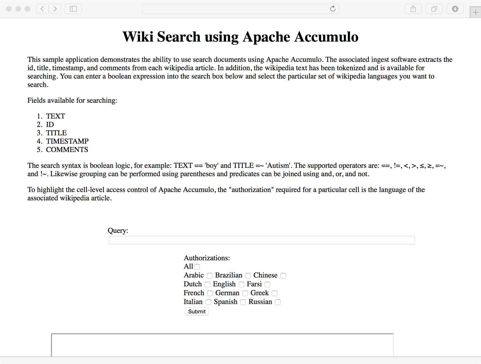
Figure 8-2. The Wikisearch UI
This example uses the Apache Commons JEXL library to create a query language. The supported JEXL operators include:
-
== -
!= -
< -
<= -
> -
>= -
=~ -
!~ -
and -
or
We’ll do a search for documents that contain both the words old and man:
TEXT == 'old' and TEXT == 'man'
This returns the results in Figure 8-3.

Figure 8-3. Search results
The logs show that there were 986 matching entries for this query:
HTML query: TEXT == 'old' and TEXT == 'man'
Connecting to [instanceName = koverse, zookeepers = koversevm:2181,
    username = root].
986 matching entries found in optimized query.
AbstractQueryLogic: TEXT == 'old' and TEXT == 'man' 2.63
  1) parse query 0.00
  2) query metadata 0.01
  3) full scan query 0.00
  3) optimized query 2.62
  1) process results 0.14
      1) query global index 0.02
1976233182 Query completed.
We’ll try adding another search term, sea:
TEXT == 'old' and TEXT == 'man' and TEXT == 'sea'
This returns the results in Figure 8-4.
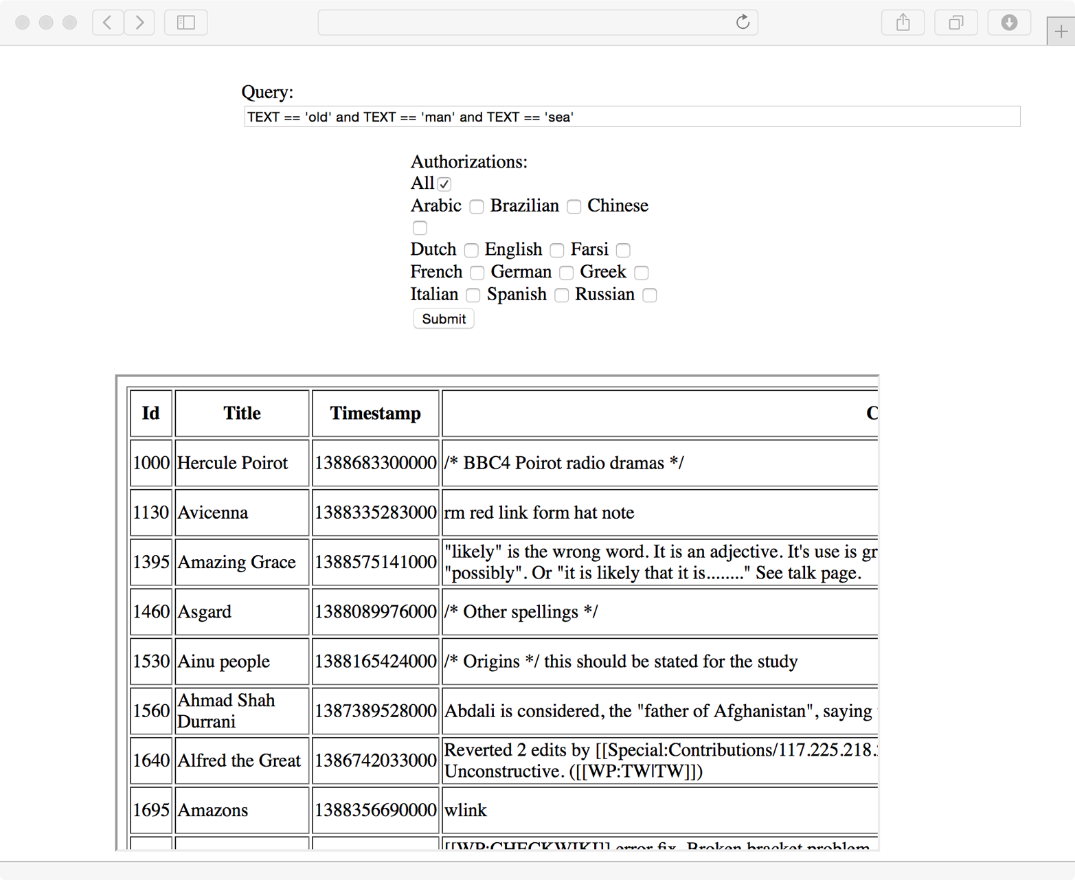
Figure 8-4. Refined search results
This cuts down the matching entries to only 339:
HTML query: TEXT == 'old' and TEXT == 'man' and TEXT == 'sea'
Connecting to [instanceName = koverse, zookeepers = koversevm:2181,
    username = root].
339 matching entries found in optimized query.
Designing Row IDs
Row IDs are the most powerful elements of the Accumulo data model because they determine the primary sort order of all the data. Here we discuss considerations for designing good row IDs, along with a few issues that can arise and methods for addressing them.
Lexicoders
The first place to look for help in designing row IDs that sort properly is Lexicoders. Lexicoders are a set of classes designed to help convert a variety of object types into byte arrays that preserve the native sort order of the objects. We introduce Lexicoders in “Using Lexicoders in indexing” for helping sort various types of objects.
Composite Row IDs
When you construct row IDs that consist of multiple elements, it is necessary to use delimiters in order to have rows sorted hierarchically, such that all of the rows that begin with one element are sorted before the first row of the next first-place element appears.
For example, if we want to sort data by first name then secondarily by last name, we need a delimiter to ensure that if we read only first names we see them all in order regardless of what last names might follow each first name. Without a delimiter we can run into the following situation:
bobanderson
bobbyanderson
bobjones
In this case “bob anderson” should be followed by “bob jones,” but because we are missing a delimiter, “bobby anderson” appears between them. Using a delimiter we get the desired sort order:
bob_anderson
bob_jones
bobby_anderson
Because the delimiter, in this case an underscore, sorts before the third b in “bobby,” all first names with four or more letters are sorted after all the appearances of “bob.”
An effective delimiter should be a character that sorts before any characters that are likely to appear in the elements of a row ID.
The null character 0 can be used if necessary.
Composite row IDs may be human-readable enough as-is.
If not, custom Formatters can be written to make viewing them easier.
See “Human-Readable Versus Binary Values and Formatters”.
The ListLexicoder and PairLexicoder can help in designing composite row IDs.
Key Size
As mentioned in “Constraints”, Accumulo 1.6 has a constraint added to new tables that the complete key be smaller than 1 MB. Keep in mind that the complete key includes the row ID, column family, column qualifier, visibility, and timestamp. Keeping the key under 1 MB is a best practice for all versions of Accumulo.
Avoiding Hotspots
In many table designs, hotspots can arise as the result of uneven distribution of row IDs, which often arises from skew in the source data. A common example is that of time-ordered row IDs, which we addressed by introducing a fixed number of bucket IDs as prefixes to spread newly written data across multiple parts of the table. We discuss avoiding hotspots in that we discuss in “Time-Ordered Data”.
Other examples include frequently appearing items in data sets, such as very frequent words appearing in textual data, highly populated areas in geospatial data, and temporal spikes in time series data. These can all cause an inordinate amount of data to be sent to one server, undermining the effectiveness of the distributed system.
Hotspots can involve simply one server being many times busier than all the others. They also can involve contention over individual rows and the creation of very large rows, due to Accumulo’s control over concurrent access to each individual row. In either case, the general approach is to alter the row IDs to either spread them over a larger portion of the table and therefore over a larger number of servers, or to simply break up highly contested rows into multiple rows to eliminate contention and overly large rows.
In the case of many writes ending up going to one server, introducing some sort of prefix in front of the row ID can cause the writes to be sent to as many servers as there are unique prefixes. An example of this is the fixed buckets that we discuss in “Time-Ordered Data” and also in document-partitioned indexes in “Index Partitioned by Document”.
An example of breaking up contentious rows is to append a suffix to the row ID. Multiple writes to the same data then end up going to different row IDs while keeping the rows next to each other, preserving scan order. One example is in indexing the word the, which appears more than any other word in English documents. Instead of simply indexing the word the, you can attach a random suffix to the word the like this:
the_023012
the_034231
the_323133
the_812500
This way multiple writers can still index the word the and avoid contention because they are technically writing to different rows. In addition, the tablet containing the word the can now be split into multiple tablets hosted on multiple servers, which would not be possible if all instances of the word the were indexed into the same row.
Scanners only need to be modified to begin at the first random suffix and end at the last:
'the_' to 'the`'
Other strategies for avoiding hotspots in indexed data involve indexing pairs of words when one word is very frequent. Instead of indexing the we would index the_car, the_house, etc. This has the advantage of making it easier to find records containing two words when one word is very frequent, while preserving the ability to retrieve all records containing just the frequent word.
Sometimes, very frequent items are not of interest to an application and can simply be omitted from the index. Apache Lucene and other indexing libraries often employ stop lists, which contain very frequent words that can be skipped when individual words in a document are indexed.
Some users have used Accumulo combiners to keep track of how many times a term appears in an index using a separate column family and cease to store additional terms after seeing a given number of them, as in the wikisearch example in “Full-Text Search”. This strategy is useful because it doesn’t require knowing the frequent terms beforehand, as a stop list does. However, by itself it doesn’t prevent clients from continuing to write frequent terms that will be ignored. An index like this could be scanned periodically (perhaps using a MapReduce job) to retrieve only the highly frequent terms for the purpose of creating a stop list that clients can use.
Designing Row IDs for Consistent Updates
Accumulo is designed to split tables into tablets on row boundaries. Tablet servers will not split a row into two tablets, so each row is fully contained within one tablet. The Accumulo master ensures that exactly one tablet server will be responsible for each tablet, and therefore each row. As a result, applications can make multiple changes to the data in one row simultaneously or, in database parlance, atomically, meaning that the server will never apply a portion of the changes. If something goes wrong while some changes are applied, the mutation will simply fail, the row will revert to the last consistent state, and the client process can try it again.
Applications that need to make updates to several data elements simultaneously can try to use the row construct to gather the data that needs to be changed simultaneously together under one row ID. An example is perhaps changing all of the elements of a customer address simultaneously so that the address is always valid and not some combination of an old and new address.
Sometimes grouping data that needs to be changed under a common row ID is not possible. An example is an application that needs to transfer amounts of money between accounts. This involves subtracting an amount from one account and adding it to the other account. Either both or neither of these actions should succeed. If only one succeeds, money is either created or destroyed. The pair of accounts that needs to be modified is not known beforehand and is impractical for use as a row ID.
It is possible to achieve this capability in a system based on BigTable as evidenced by Google’s Percolator paper, which describes an application layer implemented over BigTable that provides distributed atomic updates, or distributed transactions. The Fluo project is developing a framework for distributed transactions on top of Accumulo.
Also see “Transactions”.
Designing Values
Values in Accumulo are stored as byte arrays.
As such they can store any type of data, but it is up to the application developer to decide how to serialize data to be stored.
Many applications store Java String objects or other common Java objects.
There is no reason, however, that more complicated values cannot be stored.
Some developers use custom serialization code to convert their objects to values. Technologies such as Google’s Protocol Buffers, Apache Thrift, or Apache Avro have been used to generate code for serializing and deserializing complex structures to byte arrays for storage in values. Kryo is another good, Java-centric, technology for serializing Java objects extremely quickly, although the support across different versions of Kryo is limited.
Iterators can also be made to deserialize and operate on these objects.
Here we present an example using Apache Thrift. Thrift uses an IDL to describe objects and services. The IDL files are then compiled by the Thrift compiler to generate code in whatever languages are desired for implementing servers and clients. The Thrift compiler will generate serialization and deserialization code in a variety of on-the-wire formats for any data structures declared in the IDL files and will generate RPCs for any services defined. Then it is up to the application developer to implement the logic behind the RPCs.
It is possible to implement the client in one language and the server in another. This is a primary advantage to using Thrift.
In our example, we won’t create any Thrift services but will simply use Thrift to define a data structure and generate code to serialize it for storage in an Accumulo table.
Thrift structs and services are written in the IDL and are stored in a simple text file. We’ll design a struct in the Thrift IDL to store information about an order:
struct Order {
  1:i64 timestamp
  2:string product
  3:string sku
  4:float amount
  5:optional i32 discount
}
In our Order struct, we have five elements.
The first four are required and the last is optional.
The elements are numbered to support the ability to add and remove elements without breaking services that are built against older versions of these structs.
Next we’ll use the Thrift compiler to generate Java classes to serialize and deserialize this struct:
laptop:~ cd thrift
laptop:thrift compiler/cpp/thrift -gen java order.thrift
This will create a directory called gen-java that will contain our Java classes—in our case just one, Order.java. The generated file for even this simple structure is fairly long so we won’t include it here.
We can then use our newly generated class to serialize Java objects to byte arrays and back when writing to and reading from Accumulo tables:
publicclassOrderHandler{publicvoidtakeOrder(finallongcustomerID,finalStringproduct,finalDoubleamount,finalintdiscount,finalStringsku,finalBatchWriterwriter)throwsTException,MutationsRejectedException{// fill out the fields of the order objectOrderorder=newOrder();order.timestamp=newDate().getTime();order.product=product;order.sku=sku;order.amount=amount;if(discount>0){order.discount=discount;}// we use a TMemoryBuffer as our Thrift transport to write to// when serializingTMemoryBufferbuffer=newTMemoryBuffer(300);// we use the efficient TBinaryProtocol to store a compact// representation of this object.// other options include TCompactProtocol and TJSONProtocolTBinaryProtocolproto=newTBinaryProtocol(buffer);// this serialized our structure to the memory bufferorder.write(proto);byte[]bytes=buffer.getArray();// we'll store this order under a row identified by the customer IDMutationm=newMutation(Long.toString(customerID));// we generate a UUID based on the bytes of the order to distinguish// one order from another in the list of orders for each customerm.put("orders",UUID.nameUUIDFromBytes(bytes).toString(),newValue(bytes));writer.addMutation(m);}...}
When reading from this table we can use similar code to deserialize a list of Order objects from values found in the orders table:
...publicclassOrderHandler{...publicList<Order>getOrders(finallongcustomerId,finalAuthorizationsauths,finalConnectorconnector)throwsTableNotFoundException,TException{// instantiate a scanner to fetch this data from the tableScannerscanner=connector.createScanner("orders",auths);// create a range to restrict this scanner to read the given customer's infoscanner.setRange(newRange(Long.toString(customerId)));scanner.fetchColumnFamily(newText("orders"));ArrayList<Order>orders=newArrayList<>();for(Entry<Key,Value>entry:scanner){// use a TMemoryInputTransport to hold serialized bytesTMemoryInputTransportinput=newTMemoryInputTransport(entry.getValue().get());// need to use the same protocol to deserialize// as we did to serialize these objectsTBinaryProtocolproto=newTBinaryProtocol(input);Orderorder=newOrder();// deserialize the bytes in the protocol// to populate fields in the Order objectorder.read(proto);orders.add(order);}returnorders;}}
When you use an object-serialization framework, a programmatic object is converted into a byte array and stored as a single value in a table. This strategy is convenient in cases when the entire object is always retrieved.
When an application requires retrieving only a portion of an object, the fields within an object can be mapped to one key-value pair each. The advantage of splitting up the fields of an object into separate key-value pairs is that individual fields can be retrieved without having to retrieve all the fields. Locality groups can be used to further isolate groups of fields that are read together from those that are not read. See the section in “Locality Groups” on configuring locality groups.
Storing Files and Large Values
Accumulo is designed to store structured and semistructured data. It is not optimized to serve very large values, such as those that can arise from storing entire files in Accumulo. The practical limit for a value size depends on available memory, because Accumulo loads several values into memory simultaneously when servicing client requests.
When storing larger values than what comfortably fits in memory, users typically do one of two things: store the files in HDFS or some other scalable filesystem or blob store such as Amazon’s S3, or break up files into smaller chunks.
When storing files in an external filesystem or blob store, Accumulo only needs to store a pointer, such as a URL, to where the actual file can be retrieved from the external store. This has the advantage of allowing users to search and find files using Accumulo. It also inherits all the benefits of security and indexing while not having to store that actual data in Accumulo, which frees up resources for just doing lookups.
If users are more interested in retrieving specific parts of files, breaking up files into chunks and storing them in Accumulo may work better, because Accumulo can then provide the chunk of the user-requested file in one request rather than looking up the file pointer in Accumulo and fetching the file it from an external system. Files broken up into chunks can still cause problems when many chunks are retrieved simultaneously, because they can overwhelm available memory.
The Accumulo documentation includes an example of storing files as well as some discussion.
Users have contributed some example techniques for doing this.
All of this logic is managed in an application or service layer implemented above Accumulo.
Human-Readable Versus Binary Values and Formatters
In some cases it is convenient to store values in a format that is readable by humans. For example, debugging becomes easier, and viewing data in the Accumulo shell is possible.
In some cases, values are stored in human-readable form, such as UTF8 strings, and are converted to binary on the fly for operations, then converted back to human-readable values before they’re written back to the table. One example is that of storing numbers as strings in a table configured to sum the numerical values in those strings. In this case, the iterator that performs the summation is responsible for converting strings into Long or Double objects before summing them together, and then converting them back into String objects before outputting them to be sent either to the user or to the disk for storage.
The provided SummingCombiner can be configured to do this for strings, or to simply treat values as Long objects.
Many applications can be made more efficient by using binary values.
In this case, however, values are no longer easily read in the shell.
To make debugging and viewing binary values easier, users can create a custom Formatter by implementing org.apache.accumulo.core.util.format.Formatter.
This will allow the shell to display otherwise unreadable keys and values using some human-readable representation:
packageorg.apache.accumulo.examples;/*** this is an example formatter that only shows a deserialized value* and not the key*/publicclassExampleFormatterimplementsFormatter{privateIterator<Entry<Key,Value>>iter;@Overridepublicvoidinitialize(Iterable<Map.Entry<Key,Value>>scanner,booleanincludeTimestamps){iter=scanner.iterator();}@OverridepublicbooleanhasNext(){returniter.hasNext();}@OverridepublicStringnext(){Entry<Key,Value>n=iter.next();byte[]bytes=n.getValue().getBytes();// deserializeStrings=myDeserializationFunction(bytes);returns;}@Overridepublicvoidremove(){}privateStringmyDeserializationFunction(byte[]bytes){...}}
Formatters can be configured on a per-table basis by setting the table.formatter option.
Customer formatters only need to be included on the CLASSPATH when you run the shell.
The shell also makes it easy to configure formatters via the formatter command.
To add a formatter:
user@accumulo> table myTable
user@accumulo myTable> scan
user@accumulo> formatter -f org.apache.accumulo.examples.ExampleFormatter
    -t myTable
user@accumulo> scan
user@accumulo> formatter -r -t myTable
Designing Authorizations
Authorization tokens can represent any attribute or class of the data or of users. A short example of a token based on the data may be useful.
In many industries some data needs to be stored that represents information that can be used to identify an individual. This kind of data is typically referred to as Personally Identifiable Information (PII). There are guidelines and laws in the United States and other countries for how to protect PII. Other fields related to this individual might be less sensitive if the fields containing PII are omitted. Often groups such as analysts and researchers need access to these other fields but not the PII, so that they can find relationships and causes in activities and conditions.
Information such as a name, home address, and date of birth are just a few of the types of fields that are deemed PII. It could be useful to label data in these fields with the fact that it is considered PII. We could simply define a token called pii and require that users possess this token in order to read PII data. The definition of information considered PII may change, but it is not likely to change quickly. The set of users that are authorized to see PII data may change quickly, so we keep this mapping in an external system.
Besides attributes of the data to create tokens like PII, a common pattern is to label data based on the general purpose of its existence. Some fields may exist only to express how data travels within the organization, which may be sensitive and is only useful for internal debugging or auditing. This data can be labeled as for internal use only or that it exists only for auditing. We can create tokens for each of these, perhaps debug and audit.
Finally, it is common to label data based on a well-defined role in an organization that represents a group of people who need to work with it. The relationship of data to these groups is often slow-changing, though the membership of individual users in each group is often highly dynamic. Tokens that represent groups such as these may include such things as administration, billing, or research to denote the role that requires access to the data.
When a field has more than one characteristic, we can combine these tokens using & or |, which are Boolean operators representing that both tokens are required (logical AND) or that just one or both are required (logical OR), respectively.
Caution
If you are upgrading to Accumulo 1.5 or later, the API for authorizations has changed slightly.
The toString() method no longer calls the serialize() method.
The serialize() method now Base64-encodes the auths array.
Be sure to test these changes thoroughly as you upgrade.
When you consider granting authorizations to users, it is suggested that you do not use the root for anything other than table manipulation—such as creating tables and granting privileges—and that you do not give the root user any security labels. By following this suggestion, you force developers and system admins to log in as the correct user to access data.
For more on the relationship between user accounts and authorizations, see “An Example of Using Authorizations”.
Designing Column Visibilities
Once the notion of which authorization tokens might be needed is addressed, we next need to decide how to apply those tokens in column visibilities. Recall that the Accumulo data model allows a security label to be stored as part of each key. Security labels are stored in the part of the key called the column visibility (Figure 8-5).
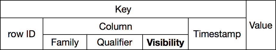
Figure 8-5. Accumulo data model
Accumulo’s security labels are designed to be flexible to meet a variety of needs. However, a result of this flexibility is that the way to define tokens and combine them into labels isn’t always obvious.
There are several things to keep in mind when designing security labels. First is which attributes of the data define the sensitivity thereof:
-
Is every record as sensitive as every other?
-
Are some fields more sensitive than others?
Second is what requirements relate to accessing the data:
-
Do users need to be granted permission before being able to read particular data elements?
-
Is access based on job role?
-
How quickly do access control needs change?
Column visibilities are designed to not be changed often.
In fact, it is impossible to actually change the column visibility stored in the key.
Rather, users have to delete the old key and write a new key and value with a different column visibility. The VersioningIterator does not help us here, because two keys that differ only by their column visibility are considered to be different keys by the VersioningIterator.
A bigger issue in trying to change column visibilities is that there can be many billions or trillions of key-value pairs, and if regular changes in column visibilities are required to support changes in access control, many new-key value pairs must be written to suppress older versions of the data. For a nontrivial amount of data, this is not tractable.
For this reason it is generally recommended to label data with attributes of the data or long-standing use cases of the data, using tokens that describe attributes of the data or groups of users that are not likely to change frequently, if ever, and then to assign tokens to individual users in order to grant access. This mapping of users to tokens is always stored in some external system such as an LDAP server. As such, the user-token mappings can be changed rapidly without the need to rewrite any data in Accumulo.