
Chapter 2
Chapter Contents
2.1 The Anatomy of the Hearing System
2.3 Frequency and Pressure Sensitivity Ranges
2.4.2 Loudness of simple sounds
2.4.3 Loudness of complex sounds
2.5 Noise-induced Hearing Loss
2.6 Perception of Sound Source Direction
2.6.1 Interaural time difference (ITD)
2.6.2 Interaural intensity difference (IID)
2.6.3 Pinnae and head movement effects
Psychoacoustics is the study of how humans perceive sound. To begin our exploration of psychoacoustics it is first necessary to become familiar with the basic anatomy of the human hearing system to facilitate understanding of:
- the effect the normal hearing system has on sounds entering the ear;
- the origin of fundamental psychoacoustic findings relevant to the perception of music;
- how listening to very loud sounds can cause hearing damage; and
- some of the listening problems faced by the hearing impaired.
This chapter introduces the main anatomical structures of the human hearing system which form the path along which incoming music signals travel up to the point where the signal is carried by nerve fibers from the ear(s) to the brain. It also introduces the concept of “critical bands”, which is the single most important psychoacoustic principle for an understanding of the perception of music and other sounds in terms of pitch, loudness and timbre.
It should be noted that many of the psychoacoustic effects have been observed experimentally, mainly as a result of playing sounds that are carefully controlled in terms of their acoustic nature to panels of listeners from whom responses are monitored. These responses are often the result of comparing two sounds and indicating, for example, which is louder or higher in pitch or “brighter.” Many of the results from such experiments cannot as yet be described in terms of either where anatomically or by what physical means they occur. Psychoacoustics is a developing field of research. However, the results from such experiments give a firm foundation for understanding the nature of human perception of musical sounds, and knowledge of minimum changes that are perceived provide useful guideline bounds for those exploring the subtleties of sound synthesis.
2.1 The Anatomy of the Hearing System
The anatomy of the human hearing system is illustrated in Figure 2.1. It consists of three sections:

Figure 2.1 The main structures of the human ear showing an overall view of the outer, middle and inner ears (left) and a detailed view of the middle and inner ear (right).
- the outer ear,
- the middle ear, and
- the inner ear.
The anatomical structure of each of these is discussed below, along with the effect that each has on the incoming acoustic signal.
The outer ear (see Figure 2.1) consists of the external flap of tissue known as the “pinna” with its many grooves, ridges and depressions. The depression at the entrance to the auditory canal is known as the “concha.” The auditory canal is approximately 25–35 mm long from the concha to the “tympanic membrane,” more commonly known as the “eardrum.” The outer ear has an acoustic effect on sounds entering the ear in that it helps us both to locate sound sources and it enhances some frequencies with respect to others.
Sound localization is helped mainly by the acoustic effect of the pinna and the concha. The concha acts as an acoustic resonant cavity. The combined acoustic effects of the pinna and concha are particularly useful for determining whether a sound source is in front or behind, and to a lesser extent whether it is above or below.
The acoustic effect of the outer ear as a whole serves to modify the frequency response of incoming sounds due to resonance effects, primarily of the auditory canal whose main resonance frequency is in the region around 4 kHz.
The tympanic membrane is a light, thin, highly elastic structure which forms the boundary between the outer and middle ears. It consists of three layers: the outside layer which is a continuation of the skin lining of the auditory canal, the inside layer which is continuous with the mucous lining of the middle ear, and the layer in between these which is a fibrous structure which gives the tympanic membrane its strength and elasticity. The tympanic membrane converts acoustic pressure variations from the outside world into mechanical vibrations in the middle ear.
2.1.2 Middle Ear Function
The mechanical movements of the tympanic membrane are transmitted through three small bones known as “ossicles,” comprising the “malleus,” “incus” and “stapes”—more commonly known as the “hammer,” “anvil” and “stirrup”—to the oval window of the cochlea (see Figure 2.1). The oval window forms the boundary between the middle and inner ears.
The malleus is fixed to the middle fibrous layer of the tympanic membrane in such a way that when the membrane is at rest, it is pulled inwards. Thus the tympanic membrane when viewed down the auditory canal from outside appears concave and conical in shape. One end of the stapes, the stapes footplate, is attached to the oval window of the cochlea. The malleus and incus are joined quite firmly such that at normal intensity levels they act as a single unit, rotating together as the tympanic membrane vibrates to move the stapes via a ball and socket joint in a piston-like manner. Thus acoustic vibrations are transmitted via the tympanic membrane and ossicles as mechanical movements to the cochlea of the inner ear.
The function of the middle ear is twofold: (1) to transmit the movements of the tympanic membrane to the fluid which fills the cochlea without significant loss of energy, and (2) to protect the hearing system to some extent from the effects of loud sounds, whether from external sources or the individual concerned.
In order to achieve efficient transfer of energy from the tympanic membrane to the oval window, the effective pressure acting on the oval window is arranged by mechanical means to be greater than that acting on the tympanic membrane. This is to overcome the higher resistance to movement of the cochlear fluid compared with that of air at the input to the ear. Resistance to movement can be thought of as “impedance” to movement and the impedance of fluid to movement is high compared with that of air. The ossicles act as a mechanical “impedance converter” or “impedance transformer” and this is achieved essentially by two means:
- the lever effect of the malleus and incus; and
- the area difference between the tympanic membrane and the stapes footplate.
The lever effect of the malleus and incus arises as a direct result of the difference in their lengths. Figure 2.2 shows this effect. The force at the stapes footplate relates to the force at the tympanic membrane by the ratio of the lengths of the malleus and incus as follows:

Figure 2.2 The function of the ossicles of the middle ear.
F1 × L1 = F2 × L2
where F1 = | force at tympanic membrane |
F2 = | force at stapes footplate |
L1 = | length of malleus |
and L2 = | length of incus |
Therefore:
![]()
The area difference has a direct effect on the pressure applied at the stapes footplate compared with the incoming pressure at the tympanic membrane since pressure is expressed as force per unit area as follows:
![]()
The areas of the tympanic membrane and the stapes footplate in humans are represented in Figure 2.2 as A1 and A2 respectively. The pressure at the tympanic membrane (P1) and the pressure at the stapes footplate (P2) can therefore be expressed as follows:

The forces can therefore be expressed in terms of pressures:

Substituting Equations 2.3 and 2.4 into Equation 2.1 gives:
![]()
Therefore:
![]()
Pickles (1982) describes a third aspect of the middle ear which appears relevant to the impedance conversion process. This relates to a buckling motion of the tympanic membrane itself as it moves, resulting in a twofold increase in the force applied to the malleus.
In humans, the area of the tympanic membrane (A1) is approximately 13 times larger than the area of the stapes footplate (A2), and the malleus is approximately 1.3 times the length of the incus. The buckling effect of the tympanic membrane provides a force increase by a factor of 2. Thus the pressure at the stapes footplate (P2) is about (13 × 1.3 × 2 = 33.8) times larger than the pressure at the tympanic membrane (P1).
Express the pressure ratio between the stapes footplate and the tympanic membrane in decibels.
The pressure ratio is 33.8:1. Equation 1.20 is used to convert from pressure ratio to decibels:
![]()
Substituting 33.8 as the pressure ratio gives:
20log10[33.8] = 30.6 dB
The second function of the middle ear is to provide some protection for the hearing system from the effects of loud sounds, whether from external sources or the individual concerned. This occurs as a result of the action of two muscles in the middle ear: the tensor tympani and the stapedius muscle. These muscles contract automatically in response to sounds with levels greater than approximately 75 dB(SPL) and they have the effect of increasing the impedance of the middle ear by stiffening the ossicular chain. This reduces the efficiency with which vibrations are transmitted from the tympanic membrane to the inner ear and thus protects the inner ear to some extent from loud sounds. Approximately 12–14 dB of attenuation is provided by this protection mechanism, but this is for frequencies below 1 kHz only. The names of these muscles derive from where they connect with the ossicular chain: the tensor tympani is attached to the “handle” of the malleus, near the tympanic membranes, and the stapedius muscle attached to the stapes.
This effect is known as the “acoustic reflex.” It takes some 60–120 ms for the muscles to contract in response to a loud sound. In the case of a loud impulsive sound such as the firing of a large gun, it has been suggested that the acoustic reflex is too slow to protect the hearing system. In gunnery situations, a sound loud enough to trigger the acoustic reflex, but not so loud as to damage the hearing systems, is often played at least 120 ms before the gun is fired.
2.1.3 Inner Ear Function
The inner ear consists of the snail-like structure known as the “cochlea.” The function of the cochlea is to convert mechanical vibrations into nerve firings to be processed eventually by the brain. Mechanical vibrations reach the cochlea at the oval window via the stapes footplate of the middle ear.
The cochlea consists of a tube coiled into a spiral with approximately 2.75 turns—see Figure 2.3(a). The end with the oval and round windows is the “base” and the other end is the “apex”—see Figure 2.3(b). Figure 2.3(c) illustrates the effect of slicing through the spiral vertically, and it can be seen in (d) that the tube is divided into three sections by Reissner’s membrane and the basilar membrane. The outer channels—the scala vestibuli (V) and scala tympani (T)—are filled with an incompressible fluid known as “perilymph,” and the inner channel is the scala media (M). The scala vestibuli terminates at the oval window and the scala tympani at the round window. An idealized unrolled cochlea is shown in Figure 2.3(b). There is a small hole at the apex known as the “helicotrema” through which the perilymph fluid can flow.

Figure 2.3 (a) The spiral nature of the cochlea. (b) The cochlea “unrolled.” (c) Vertical cross-section through the cochlea. (d) Detailed view of the cochlear tube.
Input acoustic vibrations result in a piston-like movement of the stapes footplate at the oval window, which moves the perilymph fluid within the cochlea. The membrane covering the round window moves to compensate for oval window movements since the perilymph fluid is essentially incompressible. Inward movements of the stapes footplate at the oval window cause the round window to move outwards, and outward movements of the stapes footplate cause the round window to move inwards. These movements cause traveling waves to be set up in the scala vestibuli which displace both Reissner’s membrane and the basilar membrane.
The basilar membrane is responsible for carrying out a frequency analysis of input sounds. In shape, the basilar membrane is both narrow and thin at the base end of the cochlea, becoming both wider and thicker along its length to the apex, as illustrated in Figure 2.4. The upper part of Figure 2.4 shows the idealized shape of the basilar membrane where it sits along the unrolled cochlea—compare with Figure 2.3(b), which illustrates that the width and depth of the basilar membrane are narrowest at the base and they increase towards the apex. The basilar membrane vibrates in response to stimulation by signals in the audio frequency range.

Figure 2.4 Idealized shape of basilar membrane as it lies in the unrolled cochlea (upper), and the basilar membrane response with frequency (lower).
Small structures respond better to higher frequencies than do large structures (compare, for example, the sizes of a violin and a double bass or the strings at the treble and bass ends of a piano). The basilar membrane therefore responds best to high frequencies where it is narrow and thin (at the base) and to low frequencies where it is wide and thick (at the apex). Since its thickness and width change gradually along its length, input pure tones at different frequency will produce a maximum basilar membrane movement at different positions or “places” along its length.
This is illustrated in Figure 2.5 for a section of the length of the membrane. This is the basis of the “place” analysis of sound by the hearing system. The extent, or “envelope,” of basilar membrane movement is plotted against frequency in an idealized manner for five input pure tones of different frequencies. If the input sound were a complex tone consisting of many components, the overall basilar membrane response is effectively the sum of the responses for each individual component. The basilar membrane is stimulated from the base end (see Figure 2.3) which responds best to high frequencies, and it is important to note that its envelope of movement for a pure tone (or individual component of a complex sound) is not symmetrical, but that it tails off less rapidly towards high frequencies than towards low frequencies. This point will be taken up again in Chapter 5.

Figure 2.5 Idealized envelope of basilar membrane movement to sounds at five different frequencies.
The movement of the basilar membrane for input sine waves at different frequencies has been observed by a number of researchers following the pioneering work of von Békésy (1960). They have confirmed that the point of maximum displacement along the basilar membrane changes as the frequency of the input is altered. It has also been shown that the linear distance measured from the apex to the point of maximum basilar membrane displacement is directly proportional to the logarithm of the input frequency. The frequency axis in Figure 2.5 is therefore logarithmic. It is illustrated in the figure as being “back-to-front” (i.e., with increasing frequency changing from right to left, low frequency at the apex and high at the base) to maintain the left to right sense of flow of the input acoustic signal and to reinforce understanding of the anatomical nature of the inner ear. The section of the inner ear which is responsible for the analysis of low-frequency sounds is the end farthest away from the oval window, coiled into the center of the cochlear spiral.
In order that the movements of the basilar membrane can be transmitted to the brain for further processing, they have to be converted into nerve firings. This is the function of the organ of Corti, which consists of a number of hair cells that trigger nerve firings when they are bent. These hair cells are distributed along the basilar membrane and they are bent when it is displaced by input sounds. The nerves from the hair cells form a spiral bundle known as the “auditory nerve.” The auditory nerve leaves the cochlea as indicated in Figure 2.1.
2.2 Critical Bands
Section 2.1 describes how the inner ear carries out a frequency analysis of sound due to the mechanical properties of the basilar membrane and how this provides the basis behind the “place” theory of hearing. The next important aspect of the place theory to consider is how well the hearing system can discriminate between individual frequency components of an input sound. This will provide the basis for understanding the resolution of the hearing system and it will underpin discussions relating to the psychoacoustics of how we hear music, speech and other sounds.
Each component of an input sound will give rise to a displacement of the basilar membrane at a particular place, as illustrated in Figure 2.5. The displacement due to each individual component is spread to some extent on either side of the peak. Whether or not two components that are of similar amplitude and close together in frequency can be discriminated depends on the extent to which the basilar membrane displacements, due to each of the two components, are clearly separated.
Consider track 1 on the accompanying CD. Suppose two pure tones, or sine waves, with amplitudes A1 and A2 and frequencies F1 and F2 respectively are sounded together. If F1 is fixed and F2 is changed slowly from being equal to or in unison with F1 either upwards or downwards in frequency, the following is generally heard (see Figure 2.6). When F1 is equal to F2, a single note is heard. As soon as F2 is moved higher or lower than F1 a sound with clearly undulating amplitude variations known as “beats” is heard. The frequency of the beats is equal to (F2 − F1), or (F1 − F2) if F1 is greater than F2, and the amplitude varies between (A1 + A2) and (A1 − A2), or (A1 + A2) and (A2 − A1) if A2 is greater than A1. Note that when the amplitudes are equal (A1 = A2) the amplitude of the beats varies between (2 × A1) and 0.

Figure 2.6 An illustration of the perceptual changes which occur when a pure tone fixed at frequency F1 is heard combined with a pure tone of variable frequency F2.
For the majority of listeners beats are usually heard when the frequency difference between the tones is less than about 12.5 Hz, and the sensation of beats generally gives way to one of a “fused” tone which sounds “rough” when the frequency difference is increased above 15 Hz. As the frequency difference is increased further there is a point where the fused tone gives way to two separate tones but still with the sensation of roughness, and a further increase in frequency difference is needed for the rough sensation to become smooth. The smooth separate sensation persists while the two tones remain within the frequency range of the listener’s hearing.
The changes from fused to separate and from beats to rough to smooth are shown hashed in Figure 2.6 to indicate that there is no exact frequency difference at which these changes in perception occur for every listener. However, the approximate frequencies and order in which they occur is common to all listeners, and, in common with most psychoacoustic effects, average values are quoted which are based on measurements made for a large number of listeners.
The point where the two tones are heard as being separate as opposed to fused when the frequency difference is increased can be thought of as the point where two peak displacements on the basilar membrane begin to emerge from a single maximum displacement on the membrane. However, at this point the underlying motion of the membrane, which gives rise to the two peaks, causes them to interfere with each other giving the rough sensation, and it is only when the rough sensation becomes smooth that the separation of the places on the membrane is sufficient to fully resolve the two tones. The frequency difference between the pure tones at the point where a listener’s perception changes from rough and separate to smooth and separate is known as the “critical bandwidth,” and it is therefore marked CB in the figure. A more formal definition is given by Scharf (1970): “The critical bandwidth is that bandwidth at which subjective responses rather abruptly change.”
In order to make use of the notion of critical bandwidth practically, an equation relating the effective critical bandwidth to the filter center frequency was proposed by Glasberg and Moore (1990). They define a filter with an ideal rectangular frequency response curve which passes the same power as the auditory filter in question, which is known as the “equivalent rectangular bandwidth” or “ERB.” The ERB is a direct measurement of the critical bandwidth, and the Glasberg and Moore equation which allows the calculation of the ERB for any filter center frequency is as follows:
![]()
where fc = the filter center frequency in kHz
and ERB = the equivalent rectangular bandwidth in Hz Equation valid for (100 Hz < fc < 10 000 Hz)
This relationship is plotted in Figure 2.7 and lines representing where the bandwidth is equivalent to 1, 2, 3, 4, and 5 semitones (or a semitone, whole tone, minor third, major third and perfect fourth respectively) are also plotted for comparison purposes. A third octave filter is often used in the studio as an approximation to the critical bandwidth; this is shown in the figure as the 4 semitone line (there are 12 semitones per octave, so a third of an octave is 4 semitones). A keyboard is shown on the filter center frequency axis for convenience, with middle C marked with a spot.

Figure 2.7 The variation of equivalent rectangular bandwidth (ERB) with filter center frequency and lines indicating where the bandwidth would be equivalent to 1, 2, 3, 4 and 5 semitones. (Middle C is marked with a spot on the keyboard.)
Calculate the critical bandwidth at 200 Hz and 2000 Hz to three significant figures.
Using Equation 2.6 and substituting 200 Hz and 2000 Hz for fc (noting that fc should be expressed in kHz in this equation as 0.2 kHz and 2 kHz respectively) gives the critical bandwidth (ERB) as:
![]()
The change in critical bandwidth with frequency can be demonstrated if the fixed frequency F1 in Figure 2.6 is altered to a new value and the new position of CB is found. In practice, critical bandwidth is usually measured by an effect known as “masking” (see Chapter 5) in which the “rather abrupt change” is more clearly perceived by listeners.
The response characteristic of an individual filter is illustrated in the bottom curve in Figure 2.8, the vertical axis of which is marked “filter response” (notice that increasing frequency is plotted from right to left in this figure in keeping with Figure 2.5 relating to basilar membrane displacement). The other curves in the figure are idealized envelopes of basilar membrane displacement for pure tone inputs spaced by f Hz, where f is the distance between each vertical line as marked. The filter center frequency Fc Hz is indicated with an unbroken vertical line, which also represents the place on the basilar membrane corresponding to a frequency Fc Hz. The filter response curve is plotted by observing the basilar membrane displacement at the place corresponding to Fc Hz for each input pure tone and plotting this as the filter response at the frequency of the pure tone. This results in the response curve shape illustrated as follows.

Figure 2.8 Derivation of response of an auditory filter with center frequency Fc Hz based on idealized envelope of basilar membrane movement to pure tones with frequencies local to the center frequency of the filter.
As the input pure tone is raised to Fc Hz, the membrane displacement gradually increases with the less steep side of the displacement curve. As the frequency is increased above Fc Hz, the membrane displacement falls rapidly with the steeper side of the displacement curve. This results in the filter response curve as shown, which is an exact mirror image about Fc Hz of the basilar membrane displacement curve.
Figure 2.9(a) shows the filter response curve plotted with increasing frequency and plotted more conventionally from left to right in order to facilitate discussion of the psychoacoustic relevance of its asymmetric shape in Chapter 5.

Figure 2.9 (a) Idealized response of an auditory filter with center frequency Fc Hz with increasing frequency plotted in the conventional direction (left to right). (b) Idealized bank of band-pass filters model the frequency analysis capability of the basilar membrane.
The action of the basilar membrane can be thought of as being equivalent to a large number of overlapping band-pass filters, or a “bank” of band-pass filters, each responding to a particular band of frequencies (see Chapter 1). Based on the idealized filter response curve shape in Figure 2.9(a), an illustration of the nature of this bank of filters is given in Figure 2.9(b). Each filter has an asymmetric shape to its response with a steeper roll-off on the high-frequency side than on the low-frequency side; the bandwidth of a particular filter is given by the critical bandwidth (see Figure 2.7) for any particular center frequency. It is not possible to be particularly exact with regard to the extent to which the filters overlap. A common practical compromise, for example, in studio third octave graphic equalizer filter banks, is to overlap adjacent filters at the −3 dB points on their response curves.
In terms of the perception of two pure tones illustrated in Figure 2.6, the “critical bandwidth” can be thought of as the bandwidth of the band-pass filter in the bank of filters, the center frequencies of which are exactly halfway between the frequencies of the two tones. This ignores the asymmetry of the basilar membrane response (see Figure 2.5) and the consequent asymmetry in the individual filter response curve—see Figure 2.9(a)—but it provides a good working approximation for calculations. Such a filter (and others close to it in center frequency) would capture both tones while they are perceived as “beats,” “rough fused” or “rough separate,” and at the point where rough changes to smooth, the two tones are too far apart to be both captured by this or any other filter. At this point there is no single filter which captures both tones, but there are filters which capture each of the tones individually and they are therefore resolved and the two tones are perceived as being “separate and smooth.”
A musical sound can be described by the frequency components which make it up, and an understanding of the application of the critical band mechanism in human hearing in terms of the analysis of the components of musical sounds gives the basis for the study of psychoacoustics. The resolution with which the hearing system can analyze the individual components or sine waves in a sound is important for understanding psychoacoustic discussions relating to, for example, how we perceive:
- melody
- harmony
- chords
- tuning
- intonation
- musical dynamics
- the sounds of different instruments
- blend
- ensemble
- interactions between sounds produced simultaneously by different instruments.
2.3 Frequency and Pressure Sensitivity Ranges
The human hearing system is usually quoted as having an average frequency range of 20–20 000 Hz, but there can, however, be quite marked differences between individuals. This frequency range changes as part of the human aging process, particularly in terms of the upper limit which tends to reduce. Healthy young children may have a full hearing frequency range up to 20 000 Hz, but, by the age of 20, the upper limit may have dropped to 16 000 Hz. From the age of 20, it continues to reduce gradually. This is usually known as “presbyacusis,” or less commonly as “presbycusis,” and is a function of the normal aging process.
This reduction in the upper frequency limit of the hearing range is accompanied by a decline in hearing sensitivity at all frequencies with age, the decline being less for low frequencies than for high as shown in Figure 2.10 (consider track 2 on the accompanying CD). The figure also shows that this natural loss of hearing sensitivity and loss of upper frequencies is more marked for men than for women. Hearing losses can also be induced by other factors such as prolonged exposure to loud sounds (see Section 2.5), particularly with some of the high sound levels now readily available from electronic amplification systems, whether reproduced via loudspeakers or particularly via headphones.

Figure 2.10 The average effect of aging on the hearing sensitivity of women (dotted lines) and men (solid lines) usually known as “presbyacusis,” or less commonly as “presbycusis.”
The ear’s sensitivity to sounds of different frequencies varies over a vast sound pressure level range. On average, the minimum sound pressure variation which can be detected by the human hearing system around 4 kHz is approximately 10 micropascals (10 μPa), or 10−5 Pa. The maximum average sound pressure level which is heard rather than perceived as being painful is 64 Pa. The ratio between the loudest and softest is therefore:
![]()
This is a very wide range variation in terms of the numbers involved, and it is not a convenient one to work with. Therefore sound pressure level (SPL) is represented in decibels relative to 20 μPa (see Chapter 1), as dB(SPL) as follows:
![]()
where pactual = | the actual pressure level (in Pa) |
and pref = | the reference pressure level (20 μPa) |
Example 2.3
Calculate the threshold of hearing and threshold of pain in dB(SPL).
The threshold of hearing at 1 kHz is, in fact, pref which in dB(SPL) equals:

and the threshold of pain is 64 Pa which in dB(SPL) equals:

Use of the dB(SPL) scale results in a more convenient range of values (0 to 130) to consider, since values in the range of about 0 to 100 are common in everyday dealings. Also, it is a more appropriate basis for expressing acoustic amplitude values, changes in which are primarily perceived as variations in loudness since loudness perception turns out to be essentially logarithmic in nature.
The threshold of hearing varies with frequency. The ear is far more sensitive in the middle of its frequency range than at the high and low extremes. The lower curve in Figure 2.11 is the general shape of the average threshold of hearing curve for sinusoidal stimuli between 20 Hz and 20 kHz. The upper curve in the figure is the general shape of the threshold of pain, which also varies with frequency but not to such a great extent. It can be seen from the figure that the full 130 dB(SPL) range, or “dynamic range,” between the threshold of hearing and the threshold of pain exists at approximately 4 kHz, but that the dynamic range available at lower and higher frequencies is considerably less. For reference, the sound level and frequency range for both average normal conversational speech and music are shown in Figure 2.11, while Table 2.1 shows approximate sound levels of everyday sounds for reference.

Figure 2.11 The general shape of the average human threshold of hearing and the threshold of pain with approximate conversational speech and musically useful ranges.
Table 2.1 Typical sound levels in the environment
| Example sound/situation | dB(SPL) | Description |
Long range gunfire at gunner’s ear | 140 | |
Threshold of pain | 130 | Ouch! |
Jet take-off at approximately 100 m | 120 | |
Peak levels on a night club dance floor | 110 | |
Loud shout at 1 m | 100 | Very noisy |
Heavy truck at about 10 m | 90 | |
Heavy car traffic at about 10 m | 80 | |
Car interior | 70 | Noisy |
Normal conversation at 1 m | 60 | |
Office noise level | 50 | |
Living room in a quiet area | 40 | Quiet |
Bedroom at night time | 30 | |
Empty concert hall | 20 | |
Gentle breeze through leaves | 10 | Just audible |
Threshold of hearing for a child | 0 |
2.4 Loudness Perception
Although the perceived loudness of an acoustic sound is related to its amplitude, there is not a simple one-to-one functional relationship. As a psychoacoustic effect it is affected by both the context and nature of the sound. It is also difficult to measure because it is dependent on the interpretation by listeners of what they hear. It is neither ethically appropriate nor technologically possible to put a probe in the brain to ascertain the loudness of a sound.
In Chapter 1 the concepts of the sound pressure level and sound intensity level were introduced. These were shown to be approximately equivalent in the case of free space propagation in which no interference effects were present. The ear is a pressure sensitive organ that divides the audio spectrum into a set of overlapping frequency bands whose bandwidth increases with frequency. These are both objective descriptions of the amplitude and the function of the ear. However, they tell us nothing about the perception of loudness in relation to the objective measures of sound amplitude level. Consideration of such issues will allow us to understand some of the effects that occur when one listens to musical sound sources.
The pressure amplitude of a sound wave does not directly relate to its perceived loudness. In fact it is possible for a sound wave with a larger pressure amplitude to sound quieter than a sound wave with a lower pressure amplitude. How can this be so? The answer is that the sounds are at different frequencies and the sensitivity of our hearing varies as the frequency varies. Figure 2.12 shows the equal loudness contours for the human ear. These contours, originally measured by Fletcher and Munson (1933) and by others since, represent the relationship between the measured sound pressure level and the perceived loudness of the sound. The curves show how loud a sound must be in terms of the measured sound pressure level to be perceived as being of the same loudness as a 1 kHz tone of a given level. There are two major features to take note of, which are discussed below.

Figure 2.12 Equal loudness contours for the human ear.
The first is that there are some humps and bumps in the contours above 1 kHz. These are due to the resonances of the outer ear. Within the outer ear there is a tube about 25 mm long with one open and one closed end. This will have a first resonance at about 3.4 kHz and, due to its non-uniform shape, a second resonance at approximately 13 kHz, as shown in the figure. The effect of these resonances is to enhance the sensitivity of the ear around the resonant frequencies. Note that because this enhancement is due to an acoustic effect in the outer ear it is independent of signal level.
The second effect is an amplitude dependence of sensitivity which is due to the way the ear transduces and interprets the sound and, as a result, the frequency response is a function of amplitude. This effect is particularly noticeable at low frequencies but there is also an effect at higher frequencies. The net result of these effects is that the sensitivity of the ear is a function of both frequency and amplitude. In other words the frequency response of the ear is not flat and is also dependent on sound level. Therefore two tones of equal sound pressure level will rarely sound equally loud. For example, a sound at a level which is just audible at 20 Hz would sound much louder if it was at 4 kHz. Tones of different frequencies therefore have to be at different sound pressure levels to sound equally loud and their relative loudness will also be a function of their absolute sound pressure levels.
The loudness of sine wave signals, as a function of frequency and sound pressure levels, is given by the “phon” scale. The phon scale is a subjective scale of loudness based on the judgments of listeners to match the loudness of tones to reference tones at 1 kHz. The curve for N phones intersects 1 kHz at N dB(SPL) by definition, and it can be seen that the relative shape of the phon curves flattens out at higher sound levels, as shown in Figure 2.12. The relative loudness of different frequencies is not preserved, and therefore the perceived frequency balance of sound varies as the listening level is altered. This is an effect that we have all heard when the volume of a recording is turned down and the bass and treble components appear suppressed relative to the midrange frequencies, and the sound becomes “duller” and “thinner.” Ideally we should listen to reproduced sound at the level at which it was originally recorded. However, in most cases this would be antisocial, especially as much rock material is mixed at levels in excess of 100 dB(SPL)!
In the early 1970s hi-fi manufacturers provided a “loudness” button which put in a bass and treble boost in order to flatten the Fletcher–Munson curves, and so provide a simple compensation for the reduction in hearing sensitivity at low levels. The action of this control was wrong in two important respects:
- Firstly, it directly used the equal loudness contours to perform the compensation, rather than the difference between the curves at two different absolute sound pressure levels, which would be more accurate. The latter approach has been used in professional products to allow nightclubs to achieve the equivalent effect of a louder replay level.
- Secondly, the curves are a measure of the equal loudness for sine waves at a similar level. Real music on the other hand consists of many different frequencies at many different amplitudes and does not directly follow these curves as its level changes. We shall see later how we can analyze the loudness of complex sounds. In fact because the response of the ear is dependent on both absolute sound pressure level and frequency it cannot be compensated for simply by using treble and bass boost.
These effects make it difficult to design a meter which will give a reading which truly relates to the perceived loudness of a sound, so an instrument which gives an approximate result is usually used. This is achieved by using the sound pressure level but frequency weighting it to compensate for the variation of sensitivity of the ear as a function of frequency. Clearly the optimum compensation will depend on the absolute value of the sound pressure level being measured and so some form of compromise is necessary.
Figure 2.13 shows two frequency weightings which are commonly used to perform this compensation—termed “A” and “C” weightings. The “A” weighting is most appropriate for low amplitude sounds as it broadly compensates for the low-level sensitivity versus frequency curve of the ear. The “C” weighting on the other hand is more suited to sound at higher absolute sound pressure levels and because of this is more sensitive to low-frequency components than the “A” weighting. The sound levels measured using the “A” weighting are often given in the unit dBA, and levels using the “C” weighting in dBA. Despite the fact that it is most appropriate for low sound levels, and is a reasonably good approximation there, the “A” weighting is now recommended for any sound level in order to provide a measure of consistency between measurements.

Figure 2.13 The frequency response of “A” and “C” weightings.
The frequency weighting is not the only factor which must be considered when using a sound level meter. In order to obtain an estimate of the sound pressure level it is necessary to average over at least one cycle, and preferably more, of the sound waveform. Thus most sound level meters have slow and fast time response settings. The slow time response gives an estimate of the average sound level whereas the fast response tracks more rapid variations in the sound pressure level.
Sometimes it is important to be able to calculate an estimate of the equivalent sound level experienced over a period of time. This is especially important when measuring people’s noise exposure in order to see if they might suffer noise-induced hearing loss. This cannot be done using the standard fast or slow time responses on a sound level meter; instead a special form of measurement known as the “Leq” (pronounced L E Q) measurement is used.
This measure integrates the instantaneous squared pressure over some time interval, such as 15 min or 8 h, and then takes the square root of the result. This provides an estimate of the root mean square level of the signal over the time period of the measurement and so gives the equivalent sound level for the time period. That is, the output of the Leq measurement is the constant sound pressure level, which is equivalent to the varying sound level over the measurement period. The Leq measurement also provides a means of estimating the total energy in the signal by squaring its output. A series of Leq measurements over short times can also be easily combined to provide a longer time Leq measurement by simply squaring the individual results, adding them together, and then taking the square root of the result, as shown in Equation 2.7.

This extendibility makes the Leq measurement a powerful method of noise monitoring. As with a conventional instrument, the “A” or “C” weightings can be applied.
2.4.2 Loudness of Simple Sounds
In Figure 2.10 the two limits of loudness are illustrated: the threshold of hearing and the threshold of pain. As we have already seen, the sensitivity of the ear varies with frequency and therefore so does the threshold of hearing, as shown in Figure 2.14. The peak sensitivities shown in this figure are equivalent to a sound pressure amplitude in the sound wave of 10 μPa or about –6 dB(SPL). Note that this is for monaural listening to a sound presented at the front of the listener. For sounds presented on the listening side of the head there is a rise in peak sensitivity of about 6 dB due to the increase in pressure caused by reflection from the head. There is also some evidence that the effect of hearing with two ears is to increase the sensitivity by between 3 and 6 dB.

Figure 2.14 The threshold of hearing as a function of frequency.
At 4 kHz, which is about the frequency of the sensitivity peak, the pressure amplitude variations caused by the Brownian motion of air molecules, at room temperature and over a critical bandwidth, correspond to a sound pressure level of about −23 dB. Thus the human hearing system is close to the theoretical physical limits of sensitivity. In other words there would be little point in being much more sensitive to sound, as all we would hear would be a “hiss” due to the thermal agitation of the air! Many studio and concert hall designers now try to design the building such that environmental noise levels are lower than the threshold of hearing, and so are inaudible.
The second limit is the just noticeable change in amplitude. This is strongly dependent on the nature of the signal, its frequency, and its amplitude. For broad-band noise the just noticeable difference in amplitude is 0.5 to 1 dB when the sound level lies between 20 and 100 dB(SPL) relative to a threshold of 0 dB(SPL). Below 20 dB(SPL) the ear is less sensitive to changes in sound level. For pure sine waves, however, the sensitivity to change is markedly different and is a strong function of both amplitude and frequency. For example, at 1 kHz the just noticeable amplitude change varies from 3 dB at 10 dB(SPL) to 0.3 dB at 80 dB(SPL).
This variation occurs at other frequencies as well but in general the just noticeable difference at other frequencies is greater than the values for 1–4 kHz. These different effects make it difficult to judge exactly what difference in amplitude would be noticeable as it is clearly dependent on the precise nature of the sound being listened to. There is some evidence that once more than a few harmonics are present the just noticeable difference is closer to the broad-band case, of 0.5–1 dB, rather than the pure tone case. As a general rule of thumb the just noticeable difference in sound level is about 1 dB.
The mapping of sound pressure change to loudness variation for larger changes is also dependent on the nature of the sound signal. However, for broad-band noise, or sounds with several harmonics, it is generally accepted that a change of about 10 dB in SPL corresponds to a doubling or halving of perceived loudness. However, this scaling factor is dependent on the nature of the sound, and there is some dispute over both its value and its validity.
Example 2.4
Calculate the increase in the number of violinists required to double the loudness of a string section, assuming all the violinists play at the same sound level.
From Chapter 1 the total level from combining several uncorrelated sources is given by:
![]()
This can be expressed in terms of the SPL as:
SPLN uncorrelated = SPLsingle source + 10log10(N)
In order to double the loudness we need an increase in SPL of 10 dB. Since 10 log(10) = 10, ten times the number of sources will raise the SPL by 10 dB.
Therefore we must increase the number of violinists in the string section by a factor of ten in order to double their volume.
As well as frequency and amplitude, duration also has an effect on the perception of loudness, as shown in Figure 2.15 for a pure tone. Here we can see that once the sound lasts more than about 200 milliseconds then its perceived level does not change. However, when the tone is shorter than this the perceived amplitude reduces. The perceived amplitude is inversely proportional to the length of the tone burst. This means that when we listen to sounds which vary in amplitude the loudness level is not perceived significantly by short amplitude peaks, but more by the sound level averaged over 200 milliseconds.

Figure 2.15 The effect of tone duration on loudness.
2.4.3 Loudness of Complex Sounds
Unlike tones, real sounds occupy more than one frequency. We have already seen that the ear separates sound into frequency bands based on critical bands. The brain seems to treat sounds within a critical band differently to those outside its frequency range and there are consequential effects on the perception of loudness.
The first effect is that the ear seems to lump all the energy within a critical band together and treat it as one item of sound. So when all the sound energy is concentrated within a critical band the loudness is proportional to the total intensity of the sound within the critical band. That is:
![]()
where P1−n = | the pressures of the n individual frequency components |
As the ear is sensitive to sound pressures, the sound intensity is proportional to the square of the sound pressures, as discussed in Chapter 1. Because the acoustic intensity of the sound is also proportional to the sum of the squared pressure, the loudness of a sound within a critical band is independent of the number of frequency components so long as their total acoustic intensity is constant. When the frequency components of the sound extend beyond a critical band, an additional effect occurs due to the presence of components in other critical bands. In this case more than one critical band is contributing to the perception of loudness and the brain appears to add the individual critical band responses together. The effect is to increase the perceived loudness of the sound even though the total acoustic intensity is unchanged.
Figure 2.16 shows a plot of the subjective loudness perception of a sound at a constant intensity level as a function of the sound’s bandwidth, which illustrates this effect. In the cochlea the critical bands are determined by the place at which the peak of the standing wave occurs; therefore all energy within a critical band will be integrated as one overall effect at that point on the basilar membrane and transduced into nerve impulses as a unit. On the other hand, energy which extends beyond a critical band will cause other nerves to fire and it is these extra nerve firings which give rise to an increase in loudness.

Figure 2.16 The effect of tone bandwidth on loudness.
The interpretation of complex sounds which cover the whole frequency range is further complicated by psychological effects, in that a listener will attend to particular parts of the sound, such as the soloist, or conversation, and ignore or be less aware of other sounds, and will tend to base their perception of loudness on what they have attended to.
Duration also has an effect on the perception of the loudness of complex tones in a similar fashion to that of pure tones. As is the case for pure tones, complex tones have an amplitude which is independent of duration once the sound is longer than about 200 milliseconds, and is inversely proportionate to duration when the duration is less than this.
2.5 Noise-Induced Hearing Loss
The ear is a sensitive and accurate organ of sound transduction and analysis. However, the ear can be damaged by exposure to excessive levels of sound or noise. This damage can manifest itself in two major forms:
- A loss of hearing sensitivity: The effect of noise exposure causes the efficiency of the transduction of sound into nerve impulses to reduce. This is due to damage to the hair cells in each of the organs of Corti. Note this is different from the threshold shift due to the acoustic reflex, which occurs over a much shorter time period and is a form of built-in hearing protection. This loss of sensitivity manifests itself as a shift in the threshold of hearing of someone who has been exposed to excessive noise, as shown in Figure 2.17. This shift in the threshold can be temporary, for short times of exposures, but ultimately it becomes permanent as the hair cells are permanently flattened as a result of the damage, due to long-term exposure, which does not allow them time to recover.
- A loss of hearing acuity: This is a more subtle effect, but in many ways is more severe than the first effect. We have seen that a crucial part of our ability to hear and analyze sounds is our ability to separate out the sounds into distinct frequency bands, called critical bands. These bands are very narrow. Their narrowness is due to an active mechanism of positive feedback in the cochlea which enhances the standing wave effects mentioned earlier. This enhancement mechanism is very easily damaged; it appears to be more sensitive to excessive noise than the main transduction system. The effect of the damage though is not just to reduce the threshold but also to increase the bandwidth of our acoustic filters, as shown in idealized form in Figure 2.18. This has two main effects: firstly, our ability to separate out the different components of the sound is impaired, and this will reduce our ability to understand speech or separate out desired sound from competing noise. Interestingly it may well make musical sounds that were consonant more dissonant because of the presence of more than one frequency harmonic in a critical band; this will be discussed in Chapter 3. The second effect is a reduction in the hearing sensitivity, also shown in Figure 2.18, because the enhancement mechanism also increases the amplitude sensitivity of the ear. This effect is more insidious because the effect is less easy to measure and perceive; it manifests itself as a difficulty in interpreting sounds rather than a mere reduction in their perceived level.

Figure 2.17 The effect of noise exposure on hearing sensitivity (data from Tempest, 1985).

Figure 2.18 Idealized form of the effect of noise exposure on hearing bandwidth.
Another related effect due to damage to the hair cells is noise-induced tinnitus. Tinnitus is the name given to a condition in which the cochlea spontaneously generates noise, which can be tonal or random noises, or a mixture of the two. In noise-induced tinnitus exposure to loud noise triggers this, and, as well as being disturbing, there is some evidence that people who suffer from this complaint may be more sensitive to noise-induced hearing damage.
Because the damage is caused by excessive noise exposure, it is more likely at the frequencies at which the acoustic level at the ear is enhanced. The ear is most sensitive at the first resonance of the ear canal, or about 4 kHz, and this is the frequency at which most hearing damage first shows up. Hearing damage in this region is usually referred to as an “audiometric notch” because of its distinctive shape on an audiogram (once the results have been plotted following a hearing test); see Figure 2.19. (Hearing testing using audiograms and the dBHL scale are described in detail in Section 7.2.) This distinctive pattern is evidence that the hearing loss measured is due to noise exposure rather than some other condition, such as the inevitable high-frequency loss due to aging.

Figure 2.19 Example audiograms of normal and damaged (notched) hearing.
How much noise exposure is acceptable? There is some evidence that the levels of noise generated by our normal noisy Western society have some long-term effects because measurements on the hearing of other cultures show a much lower threshold of hearing at a given age compared with that of Westerners. However, this may be due to other factors as well, for example the level of pollution. But strong evidence exists demonstrating that exposure to noises with amplitudes of greater than 90 dBA can cause permanent hearing damage. This fact is recognized, for example, by UK legislation, which requires that the noise exposure of workers be less than this limit, known as the “second action limit.” This level has been reduced since April 2006 under European legislation to 85 dBA. If the work environment has a noise level greater than the second action limit, then employers are obliged to provide hearing protection for employees of a sufficient standard to bring the noise level at the ear below this figure. There is also a “first action level,” which is 5 dB below the second action level, and if employees are subjected to this level (now 80 dBA in Europe), then employees can request hearing protection which must be made available.
Please be aware that the regulations vary by country. Readers should check their local regulations for noise exposure in practice.
2.5.1 Integrated Noise Dose
However, in many musical situations the noise level is greater than 90 dBA for short periods. For example, the audience at a concert may well experience brief peaks above this, especially at particular instants in works such as Elgar’s Dreams of Gerontius, or Orff’s Carmina Burana. Also, in many practical industrial and social situations the noise level may be louder than the second action level of 85 dBA, in Europe, for only part of the time. How can we relate intermittent periods of noise exposure to continuous noise exposure? For example, how damaging is a short exposure to a sound of 96 dBA? The answer is to use a similar technique to that used in assessing the effect of radiation exposure, that is, “integrated dose.”
The integrated noise dose is defined as the equivalent level of the sound over a fixed period of time, which is currently 8 hours. In other words the noise exposure can be greater than the second action level provided that it is for an appropriately shorter time, which results in a noise dose that is less than that which would result from being exposed to noise at the second action level for 8 hours. The measure used is the Leq mentioned earlier and the maximum dose is 85 dB Leq over 8 hours. This means that one can be exposed to 88 dBA for 4 hours, 91 dBA for 2 hours, and so on.
Figure 2.20 shows how the time of exposure varies with the sound level on linear and logarithmic timescales for the second action level in Europe. It can be seen that exposure to extreme sound levels, greater than 100 dBA, can only be tolerated for a very short period of time, less than half an hour. There is also a limit to how far this concept can be taken because very loud sounds can rupture the eardrum causing instant, and sometimes permanent, loss of hearing.

Figure 2.20 Maximum exposure time as a function of sound level plotted on a linear scale (upper) and a logarithmic scale (lower).
This approach to measuring the noise dose takes no account of the spectrum of the sound which is causing the noise exposure, because to do so would be difficult in practice. However, it is obvious that the effect of a pure tone at 85 dBA on the ear is going to be different from the same level spread over the full frequency range. In the former situation there will be a large amount of energy concentrated at a particular point on the basilar membrane and this is likely to be more damaging than the second case in which the energy will be spread out over the full length of the membrane. Note that the specification for noise dose uses “A” weighting for the measurement which, although it is more appropriate for low rather than high sound levels, weights the sensitive 4 kHz region more strongly.
2.5.2 Protecting your Hearing
Hearing loss is insidious and permanent, and by the time it is measurable it is too late. Therefore in order to protect hearing sensitivity and acuity one must be proactive. The first strategy is to avoid exposure to excess noises. Although 85 dB(SPL) is taken as a damage threshold if the noise exposure causes ringing in the ears, especially if the ringing lasts longer than the length of exposure, it may be that damage may be occurring even if the sound level is less than 85 dB(SPL).
There are a few situations where potential damage is more likely:
- The first is when listening to recorded music through headphones, as even small ones are capable of producing damaging sound levels.
- The second is when one is playing music, with either acoustic or electric instruments, as these are also capable of producing damaging sound levels, especially in small rooms with a “live” acoustic; see Chapter 6.
In both cases the levels are under your control and so can be reduced. However, there is an effect called the acoustic reflex (see Section 2.1.2), which reduces the sensitivity of your hearing when loud sounds occur. This effect, combined with the effects of temporary threshold shifts, can result in a sound level increase spiral where there is a tendency to increase the sound level “to hear it better,” which results in further dulling, etc. The only real solution is to avoid the loud sounds in the first place. However, if this situation does occur then a rest away from the excessive noise will allow some sensitivity to return.
There are sound sources over which one has no control, such as bands, discos, nightclubs, and power tools. In these situations it is a good idea either to limit the noise dose or, better still, use some hearing protection. For example, one can keep a reasonable distance away from the speakers at a concert or disco. It takes a few days, or even weeks in the case of hearing acuity, to recover from a large noise dose so one should avoid going to a loud concert, or nightclub, every day of the week!
The authors regularly use small “in-ear” hearing protectors when they know they are going to be exposed to high sound levels, and many professional sound engineers also do the same. These have the advantage of being unobtrusive and reduce the sound level by a modest, but useful, amount (15–20 dB) while still allowing conversation to take place at the speech levels required to compete with the noise! These devices are also available with a “flat” attenuation characteristic with frequency and so do not alter the sound balance too much, and cost less than a CD recording. For very loud sounds, such as those emitted by power tools, a more extreme form of hearing protection may be required, such as headphone style ear defenders.
Your hearing is essential, and irreplaceable, for the enjoyment of music, for communicating, and for socializing with other people. Now and in the future, it is worth taking care of.
2.6 Perception of Sound Source Direction
How do we perceive the direction that a sound arrives from? The answer is that we make use of our two ears, but how? Because our two ears are separated by our head, this has an acoustic effect which is a function of the direction of the sound. There are two effects of the separation of our ears on the sound wave: firstly, the sounds arrive at different times and, secondly, they have different intensities. These two effects are quite different so let us consider them in turn.
2.6.1 Interaural Time Difference (ITD)
Consider the model of the head, shown in Figure 2.21, which shows the ears relative to different sound directions in the horizontal plane. Because the ears are separated by about 18 cm there will be a time difference between the sound arriving at the ear nearest the source and the one further away. So when the sound is off to the left the left ear will receive the sound first, and when it is off to the right the right ear will hear it first. If the sound is directly in front, or behind, or anywhere on the median plane, the sound will arrive at both ears simultaneously. The time difference between the two ears will depend on the difference in the distances that the two sounds have to travel. A simplistic view might just allow for the fact that the ears are separated by a distance d and therefore calculate the effect of angle on the relative time difference by considering only the extra length introduced due to the angle of incidence, as shown in Figure 2.22. This assumption will give the following equation for the time difference due to sound angle:

Figure 2.21 The effect of the direction of a sound source with respect to the head.

Figure 2.22 A simple model for the interaural time difference.
![]()
where Δt = | the time difference between the ears (in s) |
d = | the distance between the ears (in m) |
θ = | the angle of arrival of the sound from the median (in radians) |
and c = | the speed of sound (in ms–1) |
Unfortunately this equation is wrong. It underestimates the delay between the ears because it ignores the fact that the sound must travel around the head in order to get to them. This adds an additional delay to the sound, as shown in Figure 2.23. This additional delay can be calculated, provided one assumes that the head is spherical, by recognizing that the distance traveled around the head for a given angle of incidence is given by:

Figure 2.23 The effect of the path length around the head on the interaural time difference.
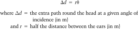
This equation can be used in conjunction with the extra path length due to the angle of incidence, which is now a function of r, as shown in Figure 2.24, to give a more accurate equation for the ITD as:

Figure 2.24 A better model for the interaural time difference.
![]()
Using this equation we can find that the maximum ITD, which occurs at 90° or (π/2 radians), is:
![]()
This is a very small delay but a variation from this to zero determines the direction of sounds at low frequencies. Figure 2.25 shows how this delay varies as a function of angle, where positive delay corresponds to a source at the right of the median plane and negative delay corresponds to a source on the left. Note that there is no difference in the delay between front and back positions at the same angle. This means that we must use different mechanisms and strategies to differentiate between front and back sounds. There is also a frequency limit to the way in which sound direction can be resolved by the ear in this way. This is due to the fact that the ear appears to use the phase shift in the wave caused by the interaural time difference to resolve the direction; that is, the ear measures the phase shift given by:
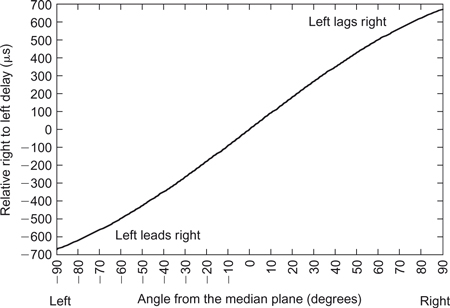
Figure 2.25 The interaural time difference (ITD) as a function of angle.
ΦITD = 2πfr (θ+ sin(θ))
where ΦITD = | the phase difference between the ears (in radians |
and f = | the frequency (in Hz) |
When this phase shift is greater than π radians (180°) there will be an unresolvable ambiguity in the direction because there are two possible angles—one to the left and one to the right—that could cause such a phase shift. This sets a maximum frequency, at a particular angle, for this method of sound localization, which is given by:
![]()
which for an angle of 90° is:
![]()
Thus for sounds at 90° the maximum frequency that can have its direction determined by phase is 743 Hz. However, the ambiguous frequency limit would be higher at smaller angles.
2.6.2 Interaural Intensity Difference (IID)
The other cue that is used to detect the direction of the sound is the differing levels of intensity that result at each ear due to the shading effect of the head. This effect is shown in Figure 2.26 which shows that the levels at each ear are equal when the sound source is on the median plane but that the level at one ear progressively reduces, and increases at the other, as the source moves away from the median plane. The level reduces in the ear that is furthest away from the source. The effect of the shading of the head is harder to calculate but experiments seem to indicate that the intensity ratio between the two ears varies sinusoidally in a frequency dependent fashion, from 0 dB up to 20 dB, depending on the sound direction, as shown in Figure 2.27.

Figure 2.26 The effect of the head on the interaural intensity difference.

Figure 2.27 The interaural intensity difference (IID) as a function of angle and frequency (data from Gulick, 1971).
However, as we saw in Chapter 1, an object is not significant as a scatterer or shader of sound until its size is about two thirds of a wavelength (![]() λ), although it will be starting to scatter an octave below that frequency. This means that there will be a minimum frequency below which the effect of intensity is less useful for localization, which will correspond to when the head is about one third of a wavelength in size (
λ), although it will be starting to scatter an octave below that frequency. This means that there will be a minimum frequency below which the effect of intensity is less useful for localization, which will correspond to when the head is about one third of a wavelength in size (![]() λ). For a head the diameter of which is 18cm, this corresponds to a minimum frequency of:
λ). For a head the diameter of which is 18cm, this corresponds to a minimum frequency of:
![]()
Thus the interaural intensity difference is a cue for direction at high frequencies whereas the interaural time difference is a cue for direction at low frequencies. Note that the crossover between the two techniques starts at about 700 Hz and would be complete at about four times this frequency at 2.8 kHz. In between these two frequencies the ability of our ears to resolve direction is not as good as at other frequencies.
2.6.3 Pinnae and Head Movement Effects
The above models of directional hearing do not explain how we can resolve front to back ambiguities or the elevation of the source. There are in fact two ways which are used by the human being to perform these tasks.
The first is to use the effect of our ears on the sounds we receive to resolve the angle and direction of the sound. This is due to the fact that sounds striking the pinnae are reflected into the ear canal by the complex set of ridges that exist on the ear. These pinnae reflections will be delayed, by a very small but significant amount, and so will form comb filter interference effects on the sound the ear receives. The delay that a sound wave experiences will be a function of its direction of arrival, in all three dimensions, and we can use these cues to help resolve the ambiguities in direction that are not resolved by the main directional hearing mechanism. The delays are very small and so these effects occur at high audio frequencies, typically above 5 kHz.
The effect is also person specific, as we all have differently shaped ears and learn these cues as we grow up. Thus we get confused for a while when we change our acoustic head shape radically, for example by cutting very long hair short. We also find that if we hear sound recorded through other people’s ears we may have a different ability to localize the sound, because the interference patterns are not the same as those for our ears. In fact, sometimes this localization capability is worse than when using our own ears and sometimes it is better.
The second, and powerful, means of resolving directional ambiguities is to move our heads. When we hear a sound that we wish to attend to, or whose direction we wish to resolve, we turn our head towards the sound and may even attempt to place it in front of us in the normal direction, where all the delays and intensities will be the same. The act of moving our head will change the direction of the sound arrival and this change of direction will depend on the sound source position relative to us. Thus a sound from the rear will move in a different direction compared with a sound in front of or above the listener. This movement cue is one of the reasons that we perceive the sound from headphones as being “in the head.” Because the sound source tracks our head movement it cannot be outside and hence must be in the head. There is also an effect due to the fact that the headphones also do not model the effect of the head. Experiments with headphone listening which correctly model the head and keep the source direction constant as the head moves give a much more convincing illusion.
2.6.4 ITD and IID Trading
Because both intensity and delay cues are used for the perception of sound source direction one might expect the mechanisms to be in similar areas of the brain and linked together. If this were the case one might also reasonably expect that there was some overlap in the way the cues were interpreted such that intensity might be confused with delay and vice versa in the brain. This allows for the possibility that the effect of one cue, for example delay, could be canceled out by the other, for example intensity. This effect does in fact happen and is known as “interaural time difference versus interaural intensity difference trading.” In effect, within limits, an interaural time delay can be compensated for by an appropriate interaural intensity difference, as shown in Figure 2.28, which has several interesting features.

Figure 2.28 Delay versus intensity trading (data from Madsen, 1990).
Firstly, as expected, time delay versus intensity trading is only effective over the range of delay times which correspond to the maximum inter aural time delay of 673 μs. Beyond this amount of delay, small intensity differences will not alter the perceived direction of the image. Instead the sound will appear to come from the source which arrives first. This effect occurs between 673 μs and 30 ms. However, if the delayed sound’s amplitude is more than 12 dB greater than the first arrival then we will perceive the direction of the sound to be towards the delayed sound. After 30 ms the delayed signal is perceived as an echo and so the listener will be able to differentiate between the delayed and undelayed sound. The implications of these results are twofold; firstly, it should be possible to provide directional information purely through either only delay cues or only intensity cues. Secondly, once a sound is delayed by greater than about 700 μs the ear attends to the sound that arrives first almost irrespective of the relative levels of the incoming sounds, although clearly if the earlier arriving sound is significantly lower in amplitude, compared with the delayed sound, then the effect will disappear.
2.6.5 The Haas Effect
The second of the ITD and IID trading effects is also known as the “Haas,” or “precedence,” effect—named after the experimenter who quantified this behavior of our ears. The effect can be summarized as follows:
- The ear will attend to the direction of the sound that arrives first and will not attend to the reflections provided they arrive within 30 ms of the first sound.
- The reflections arriving before 30 ms are fused into the perception of the first arrival. However, if they arrive after 30 ms they will be perceived as echoes.
These results have important implications for studios, concert halls and sound reinforcement systems. In essence, it is important to ensure that the first reflections arrive at the audience earlier than 30 ms to avoid them being perceived as echoes. In fact it seems that our preference is for a delay gap of less than 20 ms if the sound of the hall is to be classed as “intimate.” In sound reinforcement systems the output of the speakers will often be delayed with respect to their acoustic sound but, because of this effect, we perceive the sound as coming from the acoustic source, unless the level of sound from the speakers is very high.
2.6.6 Stereophonic Listening
Because of the way we perceive directional sound it is possible to fool the ear into perceiving a directional sound through just two loudspeakers or a pair of headphones in stereo listening. This can be achieved in basically three ways: two using loudspeakers and one using headphones. The first two ways are based on the concept of providing only one of the two major directional cues in the hearing system; that is, using either intensity or delay cues and relying on the effect of the ear’s time–intensity trading mechanisms to fill in the gaps. The two systems are as follows:
- Delay stereo: This system is shown in Figure 2.29 and consists of two omni-directional microphones spaced a reasonable distance apart and away from the performers. Because of the distance of the microphones a change in performer position does not alter the sound intensity much, but does alter the delay. So the two channels when presented over loudspeakers contain predominantly directional cues based on delay to the listener.
- Intensity stereo: This system is shown in Figure 2.30 and consists of two directional microphones placed together and pointing at the left and right extent of the performers’ positions. Because the microphones are closely spaced, a change in performer position does not alter the delay between the two sounds. However, because the microphones are directional the intensity received by the two microphones does vary. So the two channels when presented over loudspeakers contain predominantly directional cues based on intensity to the listener. Intensity stereo is the method that is mostly used in pop music production, as the pan-pots on a mixing desk, which determine the position of a track in the stereo image, vary the relative intensities of the two channels, as shown in Figure 2.31.

Figure 2.29 Delay stereo recording.

Figure 2.30 Intensity stereo recording.

Figure 2.31 The effect of the “pan-pots” in a mixing desk on intensity of the two channels.
These two methods differ primarily in the method used to record the original performance and are independent of the listening arrangement, so which method is used is determined by the producer or engineer on the recording. It is also possible to mix the two cues by using different types of microphone arrangement—for example, slightly spaced directional microphones—and these can give stereo based on both cues. Unfortunately they also provide spurious cues, which confuse the ear, and getting the balance between the spurious and wanted cues, and so providing a good directional illusion, is difficult.
- Binaural stereo: The third major way of providing a directional illusion is to use binaural stereo techniques. This system is shown in Figure 2.32 and consists of two omni-directional microphones placed on a head—real or more usually artificial—and presenting the result over headphones. The distance of the microphones is identical to the ear spacing, and they are placed on an object which shades the sound in the same way as a human head, and, possibly, torso. This means that a change in performer position provides both intensity and delay cues to the listener: the results can be very effective. However, they must be presented over headphones because any cross-ear coupling of the two channels, as would happen with loudspeaker reproduction, would cause spurious cues and so destroy the illusion. Note that this effect happens in reverse when listening to loudspeaker stereo over headphones, because the cross coupling that normally exists in a loudspeaker presentation no longer exists. This is another reason why the sound is always “in the head” when listening via conventional headphones.

Figure 2.32 Binaural stereo recording.
The main compromise in stereo sound reproduction is the presence of spurious direction cues in the listening environment because the loudspeakers and environment will all contribute cues about their position in the room, which have nothing to do with the original recording. More information about directional hearing and stereophonic listening can be found in Blauert (1997) and Rumsey (2001).
Blauert, J., 1997. Spatial Hearing: The Psychophysics of Human Sound Location, revised edn. MIT Press, Cambridge.
Fletcher, H., Munson, W., 1933. Loudness, its measurement and calculation. J. Acoust. Soc. Am. 5, 82–108.
Glasberg, B.R., Moore, B.C.J., 1990. Derivation of auditory filter shapes from notched-noise data. Hear. Res. 47, 103–138
Gulick, L.W., 1971. Hearing: Physiology and Psychophysics. Oxford University Press, Oxford, pp. 188–189.
Madsen, E.R., 1990. In: The Science of Sound. Rossing, T.D. (ed.), second edn. Addison Wesley, p. 500.
Pickles, J.O., 1982. An Introduction to the Physiology of Hearing. Academic Press, London.
Rumsey, F., 2001. Spatial Audio. Focal Press, Oxford.
Scharf, B., 1970. Critical bands. In: Tobias, J.V. (ed.), Foundations of Modern Auditory Theory, Vol. 1. Academic Press, London, pp. 159–202
Tempest, W., 1985. The Noise Handbook, (ed.) Academic press.
von Békésy, G., 1960. Experiments in Hearing. McGraw-Hill, New York.