
Recent Advances on LIP Nonlinear Filters and Their Applications
Efficient Solutions and Significance-Aware Filtering
Christian Hofmann⁎; Walter Kellermann⁎ ⁎Friedrich-Alexander-Universität Erlangen-Nürnberg, Lehrstuhl für Multimediakommunikation und Signalverarbeitung, Erlangen, Germany
Abstract
Linear-In-the-Parameters (LIP) nonlinear filters are categorized as Cascade Models (CMs) (generalizing Hammerstein models), Cascade Group Models (CGMs) (generalizing Hammerstein Group models (HGMs) and including, e.g., Volterra filters) and bilinear cascade models, where the filter output is a bilinear function of the model parameters. Time-domain and partitioned-block frequency-domain adaptation of CGMs and CMs is described and the methods for adapting bilinear cascade models are summarized as variants of the filtered-X adaptation. These models and algorithms are employed to review the Significance-Aware (SA) filtering concept, decomposing the model for the unknown system and the adaptation mechanism into synergetic subsystems to achieve high computational efficiency. In particular, the Serial SA (SSA) and Parallel SA (PSA) decomposition lead to SSA-CMs, PSA-CGMs and a novel PSA filtered-X algorithm. The main concepts described in this chapter are exemplarily compared for the challenging application of nonlinear acoustic echo cancellation. Furthermore, model structure estimation for LIP nonlinear filters based on convex filter combinations is briefly outlined and compared with SA filtering.
Keywords
Cascade models; Cascade group models; Hammerstein models; Hammerstein group models; Significance-aware filtering; SA filtering; Filtered-X
Chapter Points
- • LIP nonlinear filters with simple linear dependence on the parameters can be identified in a unified way by classical partitioned-block frequency-domain normalized least mean square algorithms.
- • Algorithms to adapt LIP nonlinear filters with bilinear dependence on parameter subsets can be treated in a unified way as filtered-X algorithms.
- • Significance-aware filtering can be applied in both cases for the efficient and effective identification of LIP nonlinear filters.
Acknowledgements
This book chapter could not have been written without the dedicated work of many former students and collaborators in the authors' research group, especially Alexander Stenger, Fabian Küch, Marcus Zeller and Luis A. Azpicueta-Ruiz.
4.1 Introduction
Linear-In-the-Parameters (LIP) nonlinear filters constitute a broad class of nonlinear systems and are used for modeling in a broad range of scientific areas, such as in biology (e.g., [1,2]), control engineering (e.g., [3]), communications (e.g., [4–6]) and in acoustic signal processing, where they are, for instance, employed for loudspeaker linearization (e.g., [7–9]) and Acoustic Echo Cancellation (AEC) (e.g., [10–16]). A nonlinear system with input ![]() and output
and output ![]() , where n is the discrete-time sample index, will be described by the input/output relation
, where n is the discrete-time sample index, will be described by the input/output relation
and will be called a memoryless nonlinearity if and only if ![]() for any n and
for any n and ![]() , where
, where ![]() is the unit impulse. Otherwise,
is the unit impulse. Otherwise, ![]() will be called a nonlinearity with memory. In both cases, a nonlinearity may either be considered as time-invariant and known, or as parametrized by a set of unknown parameters. The following treatment will focus on LIP nonlinear filters, where the output depends linearly on the parameters, e.g., on a vector a, or bilinearly on two parameter subsets, e.g., on parameter vectors
will be called a nonlinearity with memory. In both cases, a nonlinearity may either be considered as time-invariant and known, or as parametrized by a set of unknown parameters. The following treatment will focus on LIP nonlinear filters, where the output depends linearly on the parameters, e.g., on a vector a, or bilinearly on two parameter subsets, e.g., on parameter vectors ![]() and
and ![]() .
.
The adaptive identification of a parametric model for an unknown nonlinear system ![]() is illustrated in Fig. 4.1. Therein, an adaptive nonlinear filter (the parametric model) produces an estimate
is illustrated in Fig. 4.1. Therein, an adaptive nonlinear filter (the parametric model) produces an estimate ![]() for an observation
for an observation ![]() and the filter's parameters are iteratively refined (adapted) to minimize a cost function derived from the error signal
and the filter's parameters are iteratively refined (adapted) to minimize a cost function derived from the error signal ![]() , based on noisy observations
, based on noisy observations ![]() . When obtaining the observations by measuring a physical signal,
. When obtaining the observations by measuring a physical signal, ![]() may be the superposition of sensor self-noise and other processes coupling into the sensors as well.
may be the superposition of sensor self-noise and other processes coupling into the sensors as well.
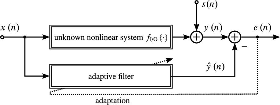
As will be explained in the following, AEC is a particularly challenging example for system identification. For AEC, ![]() in Fig. 4.1 corresponds to a microphone signal composed of local sound sources
in Fig. 4.1 corresponds to a microphone signal composed of local sound sources ![]() (e.g., the local speaker in a telephone communication) and acoustic echoes
(e.g., the local speaker in a telephone communication) and acoustic echoes ![]() from a played-back loudspeaker signal
from a played-back loudspeaker signal ![]() (e.g., the far-end speaker in a telephone communication). The AEC system aims at removing the acoustic echoes
(e.g., the far-end speaker in a telephone communication). The AEC system aims at removing the acoustic echoes ![]() from the microphone signal
from the microphone signal ![]() , using an echo signal estimate
, using an echo signal estimate ![]() . In periods of local sound source activity, the error signal
. In periods of local sound source activity, the error signal ![]() constitutes an estimate for the local sound sources
constitutes an estimate for the local sound sources ![]() . In single-talk periods where only the echo signal
. In single-talk periods where only the echo signal ![]() contributes to the microphone signal, the error signal can be employed to refine the adaptive filter. The detection of local sound sources (double-talk detection) is out of the scope of this chapter and solutions for this problem exist (e.g., [17,18]). Therefore, we will assume that no local sources are active when considering AEC, which means
contributes to the microphone signal, the error signal can be employed to refine the adaptive filter. The detection of local sound sources (double-talk detection) is out of the scope of this chapter and solutions for this problem exist (e.g., [17,18]). Therefore, we will assume that no local sources are active when considering AEC, which means ![]() .
.
AEC is a particularly challenging example for system identification due to the complex acoustic echo paths to be modeled, which typically requires nonlinear adaptive filters with large memory. Furthermore, adaptive filters have to identify a system excited by speech or audio signals (super-Gaussian, non-white and highly instationary signals) instead of signals tailored to system identification. Thus, constituting an especially challenging application, AEC will be used as a reference for evaluating the methods in this chapter. However, the models described and introduced in this chapter are not limited to AEC. Potential other applications will be highlighted at the beginning of Section 4.5, where the required terminology on nonlinear systems and their adaptation will have been established.
The organization of this chapter will be summarized in the following. After introducing the fundamental notations and terminology in the remainder of this section, state-of-the-art LIP nonlinear filters will be categorized in Section 4.2 and fundamental algorithms for parameter estimation for such filters will be presented in Section 4.3. Resulting from a unified treatment of time-domain Normalized Least Mean Square (NLMS), Partitioned-Block Frequency-domain Normalized Least Mean Square (PB-FNLMS), as well as Filtered-X (FX) algorithms for LIP nonlinear filters, a novel and efficient FX PB-FNLMS algorithm will be introduced. In Section 4.4, the recently proposed, computationally very efficient concept of Significance-Aware (SA) filtering will be summarized and a novel SA FX PB-FNLMS algorithm with even further increased efficiency will be proposed. The adaptive filtering techniques described in this chapter will be evaluated and compared in Section 4.5. Finally, similarities and differences of SA filters and nonlinear adaptive filtering techniques based on convex filter combinations for model structure estimation will be reviewed in Section 4.6, before summarizing this chapter in Section 4.7.
Notations and Fundamentals As common in system identification literature, the terms filter and system are used interchangeably. The input/output relationship of a linear, causal Finite Impulse Response (FIR) system of length L with input signal ![]() and output
and output ![]() will be written as
will be written as
where ![]() denotes the
denotes the ![]() tap of the system's Impulse Response (IR), ⁎ denotes convolution, and
tap of the system's Impulse Response (IR), ⁎ denotes convolution, and ![]() represents the scalar product between the vectors h and
represents the scalar product between the vectors h and ![]() , where
, where
denote the IR vector and the time-reversed input signal vector, respectively, and the time reversal is indicated by the caron accent. Furthermore, ![]() and
and ![]() will denote the
will denote the ![]() matrix of zeros and the
matrix of zeros and the ![]() identity matrix, respectively, and are used as components of the windowing matrices
identity matrix, respectively, and are used as components of the windowing matrices

which set the first and second half of a vector of length ![]() to zero, respectively. In addition, F will refer to the
to zero, respectively. In addition, F will refer to the ![]() unitary Discrete Fourier Transform (DFT) matrix and
unitary Discrete Fourier Transform (DFT) matrix and ![]() and
and ![]() will denote element-wise multiplication and division of the vectors
will denote element-wise multiplication and division of the vectors ![]() and
and ![]() , respectively. The element-wise magnitude square computation for the entries of a vector a will be written as
, respectively. The element-wise magnitude square computation for the entries of a vector a will be written as ![]() .
.
4.2 A Concise Categorization of State-of-the-Art LIP Nonlinear Filters
In this section, generic state-of-the-art LIP nonlinear filter structures are introduced as building blocks for the recently developed and newly proposed adaptive filtering methods in Sections 4.3 and 4.4.
4.2.1 Hammerstein Models and Cascade Models
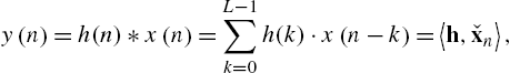
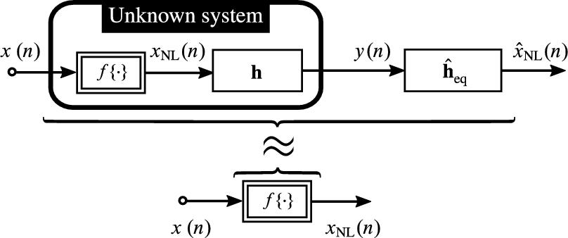
A very simple class of LIP nonlinear filters can be described with the cascade structure depicted in Fig. 4.2, where a nonlinearity ![]() is followed by a linear system with IR vector h. The output depends linearly on the parameters h of the linear system and can be expressed in the notation of Eq. (4.2) as
is followed by a linear system with IR vector h. The output depends linearly on the parameters h of the linear system and can be expressed in the notation of Eq. (4.2) as
If ![]() in Fig. 4.2 is a memoryless nonlinearity, the structure is widely known as HM [19], whereas the more general case, where
in Fig. 4.2 is a memoryless nonlinearity, the structure is widely known as HM [19], whereas the more general case, where ![]() is a nonlinearity with memory, will simply be referred to as CM in the following (the attribute nonlinear will be implied). HMs can, for instance, be employed for loudspeaker linearization (e.g., [20,21]) and AEC (e.g., [22–32]). HMs are simple and powerful models for acoustic echo paths if the major source of nonlinearity is the playback equipment (amplifiers and loudspeakers operating at the limits of their dynamic range) and can be mapped to
is a nonlinearity with memory, will simply be referred to as CM in the following (the attribute nonlinear will be implied). HMs can, for instance, be employed for loudspeaker linearization (e.g., [20,21]) and AEC (e.g., [22–32]). HMs are simple and powerful models for acoustic echo paths if the major source of nonlinearity is the playback equipment (amplifiers and loudspeakers operating at the limits of their dynamic range) and can be mapped to ![]() , while the acoustic IR (describing sound propagation through the acoustic environment) can be described by h [22].
, while the acoustic IR (describing sound propagation through the acoustic environment) can be described by h [22].
4.2.2 Hammerstein Group Models and Cascade Group Models
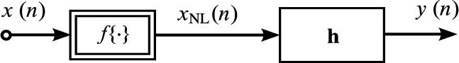
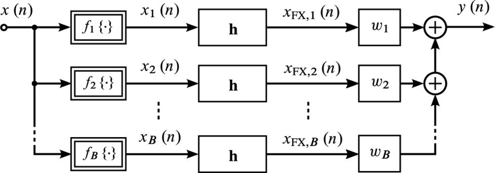
The term Cascade Group Model (CGM) will refer to models with the structure depicted in Fig. 4.3. Such CGMs are composed of B parallel branches, each of which is a nonlinear CM (see Section 4.2.1) with a branch nonlinearity ![]() and IR
and IR ![]() . For memoryless branch nonlinearities
. For memoryless branch nonlinearities ![]() , each branch becomes an HM and the entire CGM will be referred to as HGM in the following. HGMs have successfully been employed to describe both acoustic systems, e.g., in [33–37], and nonacoustic systems, e.g., [38,39]. In their treatment in the literature, HGMs have been addressed by various names, such as the Uryson model [3,39], or are simply treated as an approximation of a particular CGM. The most prominent examples of such HGM/CGM pairs are the so-called power filters [37,40,41] and Volterra filters [19]. Power filters are HGMs with monomes as branch nonlinearities
, each branch becomes an HM and the entire CGM will be referred to as HGM in the following. HGMs have successfully been employed to describe both acoustic systems, e.g., in [33–37], and nonacoustic systems, e.g., [38,39]. In their treatment in the literature, HGMs have been addressed by various names, such as the Uryson model [3,39], or are simply treated as an approximation of a particular CGM. The most prominent examples of such HGM/CGM pairs are the so-called power filters [37,40,41] and Volterra filters [19]. Power filters are HGMs with monomes as branch nonlinearities ![]() , e.g.,
, e.g.,
Volterra filters result from power filters by augmenting the latter with additional branches where the branch nonlinearities ![]() perform time-lagged products of powers of the input (time-lagged products of the power filter branch nonlinearities), e.g., the set
perform time-lagged products of powers of the input (time-lagged products of the power filter branch nonlinearities), e.g., the set

leads to a Volterra filter in Diagonal Coordinate Representation (DCR) [6]. The set of IRs ![]() of branches where
of branches where ![]() performs (potentially time-lagged) products of o input signal values is called oth-order Volterra kernel and the branches within a kernel are also termed diagonals of the respective kernel. In the aforementioned example, the second-order kernel is modeled by
performs (potentially time-lagged) products of o input signal values is called oth-order Volterra kernel and the branches within a kernel are also termed diagonals of the respective kernel. In the aforementioned example, the second-order kernel is modeled by ![]() diagonals (
diagonals (![]() ). Volterra filters are universal approximators for a large class of nonlinear systems and have therefore been applied in biology (e.g. [1]), control engineering (e.g., [3]) and communications (e.g., [4–6]), as well as in acoustic signal processing (e.g., [7–16,42,43]). Recently, HGMs and CGMs have also been realized with other sets of branch nonlinearities, such as Fourier basis functions [44], Legendre polynomials [45,46] or Chebyshev polynomials [47]. Also, Functional-Link Adaptive Filters (FLAFs) [34,35,48–50] can be viewed as HGM or CGM structures. All these models can be described by the input/output relationship
). Volterra filters are universal approximators for a large class of nonlinear systems and have therefore been applied in biology (e.g. [1]), control engineering (e.g., [3]) and communications (e.g., [4–6]), as well as in acoustic signal processing (e.g., [7–16,42,43]). Recently, HGMs and CGMs have also been realized with other sets of branch nonlinearities, such as Fourier basis functions [44], Legendre polynomials [45,46] or Chebyshev polynomials [47]. Also, Functional-Link Adaptive Filters (FLAFs) [34,35,48–50] can be viewed as HGM or CGM structures. All these models can be described by the input/output relationship
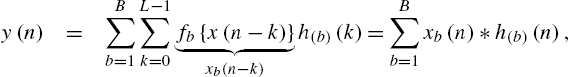
where ![]() denotes the kth tap of the linear subsystem in branch b and
denotes the kth tap of the linear subsystem in branch b and ![]() is the bth branch signal. Thus, algorithms developed for one particular realization (i.e., set of basis functions
is the bth branch signal. Thus, algorithms developed for one particular realization (i.e., set of basis functions ![]() ) of CGMs can often immediately be applied to other realizations. This holds for the adaptation algorithms for coefficient estimation described in Sections 4.3 and 4.4, as well as for the structure estimation methods outlined in Section 4.6.
) of CGMs can often immediately be applied to other realizations. This holds for the adaptation algorithms for coefficient estimation described in Sections 4.3 and 4.4, as well as for the structure estimation methods outlined in Section 4.6.
4.2.3 Bilinear Cascade Models
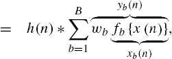
For applications where CGMs with a large number of branches are computationally too demanding, e.g., for AEC in mobile devices with very limited processing or battery power, CM-structured adaptive filters are particularly attractive. Yet, the nonlinearity itself is usually unknown. Therefore, the nonlinearity ![]() of a CM is typically modeled by a parametric preprocessor according to
of a CM is typically modeled by a parametric preprocessor according to

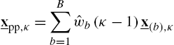
where B nonlinearities ![]() are combined with weights
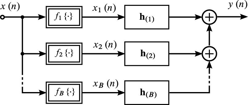
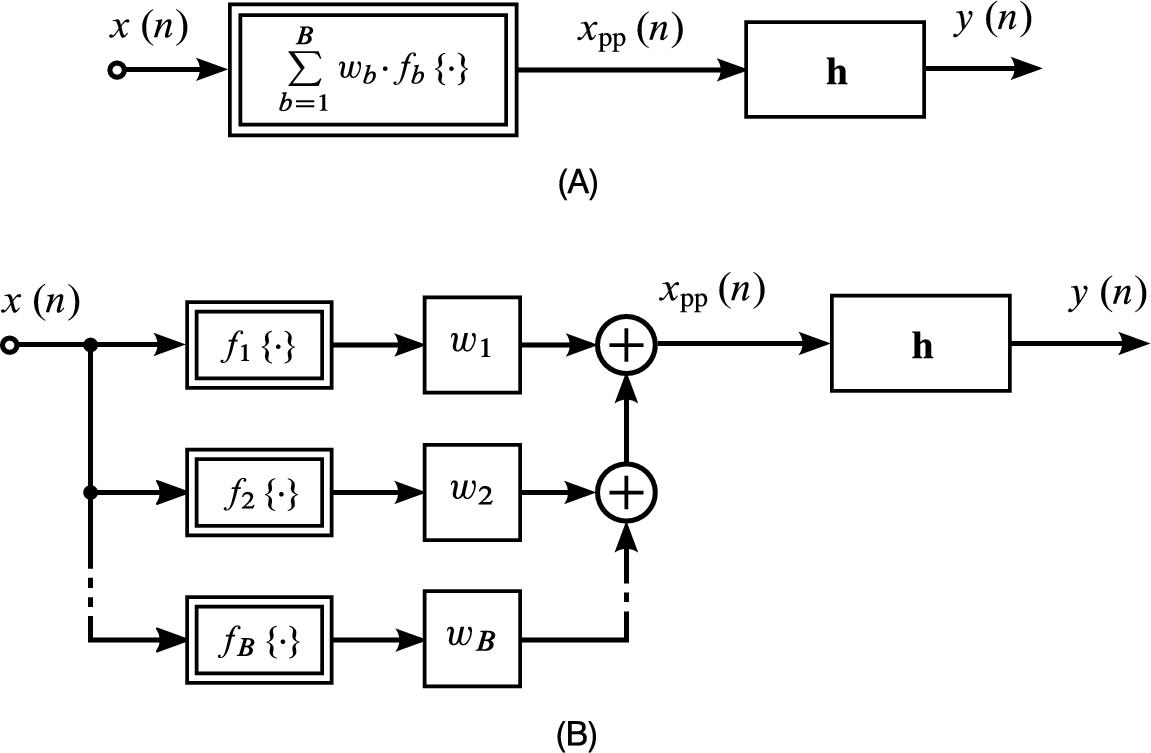
are combined with weights ![]() , which are parameters to be identified in addition to the linear subsystem. The subindex “pp” of the nonlinear preprocessor and its output signal are used to emphasize the parametrical structure of the preprocessor. The general structure of a CM with a preprocessor according to Eq. (4.8) is depicted in Fig. 4.4A. Most prominently,
, which are parameters to be identified in addition to the linear subsystem. The subindex “pp” of the nonlinear preprocessor and its output signal are used to emphasize the parametrical structure of the preprocessor. The general structure of a CM with a preprocessor according to Eq. (4.8) is depicted in Fig. 4.4A. Most prominently, ![]() are chosen as monomes [20,21,24,51–54], e.g.,
are chosen as monomes [20,21,24,51–54], e.g., ![]() , such that the nonlinearity
, such that the nonlinearity ![]() can be seen as a truncated Taylor series expansion. Fourier series- [55] and Legendre series-based approximations [28,30,31,56] have also recently been employed in AEC. Expanding the preprocessor of Fig. 4.4A in the block diagram results in Fig. 4.4B. Obviously, such a system has the input/output relationship
can be seen as a truncated Taylor series expansion. Fourier series- [55] and Legendre series-based approximations [28,30,31,56] have also recently been employed in AEC. Expanding the preprocessor of Fig. 4.4A in the block diagram results in Fig. 4.4B. Obviously, such a system has the input/output relationship
and the paths from ![]() to
to ![]() consist not only of a single linear system, but of cascades of
consist not only of a single linear system, but of cascades of ![]() (a single-tap linear system) with the linear system h. Therefore, the output of
(a single-tap linear system) with the linear system h. Therefore, the output of ![]() linearly depends on both the parameter vector
linearly depends on both the parameter vector ![]() and the parameter vector h, which is why such systems will be referred to as bilinear1 CMs in the following. Bilinearity holds regardless of
and the parameter vector h, which is why such systems will be referred to as bilinear1 CMs in the following. Bilinearity holds regardless of ![]() being memoryless or with memory and also for general linear filters with IRs
being memoryless or with memory and also for general linear filters with IRs ![]() replacing the single-tap filters
replacing the single-tap filters ![]() , resulting in CGM preprocessors.2 Thus, in the following, all considerations on simple preprocessor systems according to Fig. 4.4A translate to bilinear CMs with CGM preprocessors and vice versa, unless noted otherwise.
, resulting in CGM preprocessors.2 Thus, in the following, all considerations on simple preprocessor systems according to Fig. 4.4A translate to bilinear CMs with CGM preprocessors and vice versa, unless noted otherwise.
 instead of
  . (B) Expansion of the memoryless nonlinearity in (A), revealing a bilinear dependency of the model output
  on the parameter vectors
  and h.
4.3 Fundamental Methods for Coefficient Adaptation
The most common methods for parameter estimation for linear and LIP nonlinear filters are stochastic gradient-type algorithms, such as the Least Mean Square (LMS) algorithm or the NLMS algorithm [57]. These can be derived as an approximation of a gradient descent w.r.t. the mean squared error cost function ![]() , where
, where ![]() denotes mathematical expectation and
denotes mathematical expectation and ![]() is the error signal, computed as difference between the unknown system's output
is the error signal, computed as difference between the unknown system's output ![]() and its estimate
and its estimate ![]() , obtained with the adaptive filter (cf. Fig. 4.1). For a comprehensive treatment of different types of LMS-type algorithms, we refer to [57].
, obtained with the adaptive filter (cf. Fig. 4.1). For a comprehensive treatment of different types of LMS-type algorithms, we refer to [57].
In the following, classical system identification will be employed in Section 4.3.1 to adapt ![]() of CGMs from Section 4.2.2 (cf. Fig. 4.3). In Section 4.3.2, the filtered-X method is employed to convert the adaptation of a preprocessor system according to Section 4.2.3 (cf. Fig. 4.4) into two ordinary system identification tasks, one for
of CGMs from Section 4.2.2 (cf. Fig. 4.3). In Section 4.3.2, the filtered-X method is employed to convert the adaptation of a preprocessor system according to Section 4.2.3 (cf. Fig. 4.4) into two ordinary system identification tasks, one for ![]() and one for
and one for ![]() , by reordering
, by reordering ![]() and
and ![]() .
.
4.3.1 NLMS for Cascade Group Models
In this section, the adaptation of CGMs according to Section 4.2.2 by a time-domain and a partitioned-block frequency-domain NLMS will be described in Sections 4.3.1.1 and 4.3.1.2, respectively. Note that the branch nonlinearities will be considered as time-invariant and known, such that only the linear subsystems of ![]() of the CGMs from Section 4.2.2 are adaptive.
of the CGMs from Section 4.2.2 are adaptive.
4.3.1.1 Time-Domain NLMS
To implement and adapt a CGM, the input signal ![]() has to be mapped nonlinearly to a set of branch signals
has to be mapped nonlinearly to a set of branch signals
as inputs for the linear ![]() Multiple-Input/Single-Output (MISO) subsystem depicted in the right half of Fig. 4.3. This allows one to compute output samples
Multiple-Input/Single-Output (MISO) subsystem depicted in the right half of Fig. 4.3. This allows one to compute output samples
where ![]() is the length-L IR estimate in branch b and has been obtained at time index
is the length-L IR estimate in branch b and has been obtained at time index ![]() and where
and where ![]() is the time-reversed branch signal vector, structured analogously to Eq. (4.4). This allows one to compute the error signal
is the time-reversed branch signal vector, structured analogously to Eq. (4.4). This allows one to compute the error signal
before performing for each branch b a filter update according to
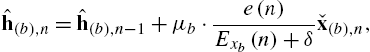
with the branch-specific adaptation step sizes ![]() , a nonnegative regularization constant δ for numerical stability and the branch signal energies
, a nonnegative regularization constant δ for numerical stability and the branch signal energies
The computational effort of such a time-domain NLMS-adaptive CGM grows linearly with the number of branches B. Note that the CGM adaptation includes the CM adaptation for ![]() and the adaptation of linear systems for
and the adaptation of linear systems for ![]() and
and ![]() .
.
4.3.1.2 Partitioned-Block Frequency-Domain NLMS
To efficiently adapt LIP nonlinear filters with a low input/output delay, Partitioned Block (PB) frequency-domain algorithms can be applied. For this purpose, a PB-FNLMS will be summarized here for CGMs.
Partitioned-Block Convolution
For partitioned-block convolution, the summation in Eq. (4.2) is split into partial sums and each partial sum (the convolution of an IR partition with an appropriately delayed segment of the input signal) is computed for M consecutive samples via fast DFT-domain convolution, like in [58–62]. This leads to block processing of the input signal ![]() with a frameshift of M samples and a frame size of
with a frameshift of M samples and a frame size of ![]() . In this notation, let the input signal vector
. In this notation, let the input signal vector ![]() at frame κ, the IR partition vector
at frame κ, the IR partition vector ![]() (containing the pth partition of h) and the output signal vector
(containing the pth partition of h) and the output signal vector ![]() at frame κ be defined as
at frame κ be defined as
respectively. Employing the length-N DFT matrix F, DFT-domain representations
can be obtained, and the output signal vector can be computed as
where ![]() results from the accumulation over all P partitions' DFT-domain products and contains cyclic convolution artifacts in its time-domain representation
results from the accumulation over all P partitions' DFT-domain products and contains cyclic convolution artifacts in its time-domain representation ![]() . Thus, the time-domain output signal vector
. Thus, the time-domain output signal vector ![]() emerges from
emerges from ![]() by premultiplication with the windowing matrix
by premultiplication with the windowing matrix ![]() , defined in Eq. (4.5).
, defined in Eq. (4.5).
Application of Partitioned-Block Convolution for Adaptive Filtering
As in the previous paragraph's partitioned convolution scheme, an adaptive CGM estimate for the linear subsystem in branch b at frame κ can be split into partitions ![]() . Their DFT-domain representations
. Their DFT-domain representations ![]() can be adapted efficiently on a frame-wise basis by an NLMS-type algorithm. To this end, branch signal vectors
can be adapted efficiently on a frame-wise basis by an NLMS-type algorithm. To this end, branch signal vectors

are determined, which contain M samples of the previous frame (upper half) and M newly computed branch signal samples (lower half), and they are transformed into the DFT domain according to
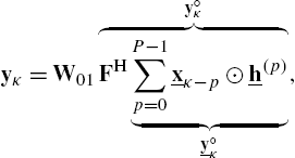
Applying the fast partitioned convolution scheme of Eq. (4.21) in all B branches and summing up all branches in the DFT domain yields the output estimate with cyclic convolution artifacts

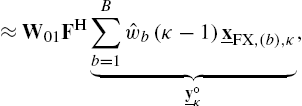
This result allows one to compute the DFT-domain error signal vector
where ![]() represents the output signal vector estimate, obtained from
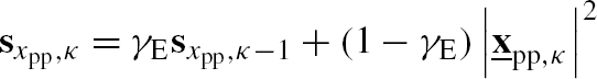
represents the output signal vector estimate, obtained from ![]() after an Inverse DFT (IDFT) and windowing. For NLMS adaptation, the DFT-domain signal energy can be estimated using a recursive averaging
after an Inverse DFT (IDFT) and windowing. For NLMS adaptation, the DFT-domain signal energy can be estimated using a recursive averaging

where ![]() is a smoothing factor (
is a smoothing factor (![]() will be assumed as default) and will be used to compute normalized branch signals
will be assumed as default) and will be used to compute normalized branch signals
where ![]() is the adaptation step size and δ is a small positive constant for numerical stability, which is added to each element of
is the adaptation step size and δ is a small positive constant for numerical stability, which is added to each element of ![]() . Based on
. Based on ![]() , the update of the filter partitions can be expressed as
, the update of the filter partitions can be expressed as
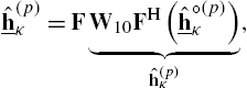
which is also known as unconstrained update in the literature [58] and where cyclic convolution artifacts lead to nonzero filter taps in the second half of ![]() . Limiting the temporal support of the partitions to M samples is possible by
. Limiting the temporal support of the partitions to M samples is possible by

and corresponds to the so-called constrained update in the literature, which is typically formulated by introducing the constraint on the update instead of the partitions (see [58]). Alternatively, a soft-partitioned update is also possible [62,63], which shapes the temporal support of ![]() by convolution in the DFT domain with a very short DFT-domain sequence in order to save the DFTs in Eq. (4.29).
by convolution in the DFT domain with a very short DFT-domain sequence in order to save the DFTs in Eq. (4.29).
Corresponding to the time-domain adaptation in Section 4.3.1.1, this section's PB-FNLMS CGM adaptation includes the CM adaptation for ![]() and the adaptation of linear systems for
and the adaptation of linear systems for ![]() and
and ![]() . Furthermore, a nonpartitioned Frequency-domain Normalized Least Mean Square (FNLMS) algorithm results from
. Furthermore, a nonpartitioned Frequency-domain Normalized Least Mean Square (FNLMS) algorithm results from ![]() . Taking the number of DFTs as measure of computational complexity, a CGM with
. Taking the number of DFTs as measure of computational complexity, a CGM with ![]() branches and
branches and ![]() partitions is about 4.3 times as complex as a linear model with
partitions is about 4.3 times as complex as a linear model with ![]() partitions (
partitions (![]() ).
).
4.3.2 Filtered-X Adaptation for Bilinear Cascade Models
In this section, the FX algorithm will first be introduced and discussed on a conceptual level for bilinear CMs, before specifying it in detail and proposing an efficient realization for CGM preprocessors with single-tap branch filters (i.e., parametric preprocessors according to Eq. (4.8)).
The Generic Filtered-X Structure FX algorithms are frequently employed in Active Noise Control (ANC) [64] for prefilter adaptation. Thereby, the FX algorithm exploits the fact that the ordering of linear time-invariant systems in a cascade can be reversed without altering the cascade's output: for the preprocessor-based CM in Fig. 4.4B, joint linearity and time invariance allow incorporating h into each of the branches, as depicted in Fig. 4.5. Therein, the prefiltered inputs to the former prefilters ![]() are often termed FX signals. The representation of the CM in Fig. 4.5 allows one to directly apply an NLMS-type adaptation algorithm for linear MISO systems from Section 4.3.1 to adapt
are often termed FX signals. The representation of the CM in Fig. 4.5 allows one to directly apply an NLMS-type adaptation algorithm for linear MISO systems from Section 4.3.1 to adapt ![]() , as their inputs are known and their combined output is directly matched to the target signal (in system identification: an unknown system's output). Mathematically, an FX LMS algorithm can also be derived directly like an LMS algorithm as stochastic gradient descent algorithm w.r.t. the partial derivative w.r.t. the prefilters. The exchange of the filtering orders results simply from an advantageous summation order in the gradient calculation. Note that adaptive filters for
, as their inputs are known and their combined output is directly matched to the target signal (in system identification: an unknown system's output). Mathematically, an FX LMS algorithm can also be derived directly like an LMS algorithm as stochastic gradient descent algorithm w.r.t. the partial derivative w.r.t. the prefilters. The exchange of the filtering orders results simply from an advantageous summation order in the gradient calculation. Note that adaptive filters for ![]() and h actually violate the time invariance required for exchanging the filter order. However, the time variance appears to be uncritical in practice, where FX algorithms have been employed for ANC for more than three decades [64,65].
and h actually violate the time invariance required for exchanging the filter order. However, the time variance appears to be uncritical in practice, where FX algorithms have been employed for ANC for more than three decades [64,65].
Review of Known Algorithms for Filtered-X Adaptation of Bilinear Cascade Models Many FX-like algorithms have been derived for the adaptation of bilinear LIP nonlinear systems but do not establish the link to the filtered-X algorithms and the exchange of filtering orders. The following description of these methods will highlight the fact that these algorithms can be viewed and implemented as FX algorithms.
In [24], the FX preprocessor adaptation was derived and applied to the adaptation of a polynomial preprocessor with ![]() —a nonadaptive offline version of this mechanism was proposed in [23], which resembles the iterative version of [51] for AutoRegressive Moving Average (ARMA) models as linear submodels. More recent work on such cascade models considered a generalization of [24] by allowing longer IRs than a single tap [37,66] or considered piece-wise linear functions for
—a nonadaptive offline version of this mechanism was proposed in [23], which resembles the iterative version of [51] for AutoRegressive Moving Average (ARMA) models as linear submodels. More recent work on such cascade models considered a generalization of [24] by allowing longer IRs than a single tap [37,66] or considered piece-wise linear functions for ![]() in conjunction with a modified joint normalization of the linear and nonlinear filter coefficients [27]. In particular, [37] employs a power filter as preprocessor to the linear subsystem. The resulting algorithm corresponds to a time-domain FX algorithm. In [66], a particular CGM preprocessor is discussed, which corresponds to a Volterra filter in triangular representation (see, e.g., [19] for the triangular representation) with memory lengths of
in conjunction with a modified joint normalization of the linear and nonlinear filter coefficients [27]. In particular, [37] employs a power filter as preprocessor to the linear subsystem. The resulting algorithm corresponds to a time-domain FX algorithm. In [66], a particular CGM preprocessor is discussed, which corresponds to a Volterra filter in triangular representation (see, e.g., [19] for the triangular representation) with memory lengths of ![]() and
and ![]() for the kernels of orders 1 and 2, respectively, and no memory at all for higher-order Volterra kernels (becoming a simple memoryless preprocessor3 for these orders). Structures similar to this preprocessor also result from the so-called EVOLutionary Volterra Estimation (EVOLVE), which will be outlined later on in Section 4.6. While evaluating their algorithm for a memoryless preprocessor (
for the kernels of orders 1 and 2, respectively, and no memory at all for higher-order Volterra kernels (becoming a simple memoryless preprocessor3 for these orders). Structures similar to this preprocessor also result from the so-called EVOLutionary Volterra Estimation (EVOLVE), which will be outlined later on in Section 4.6. While evaluating their algorithm for a memoryless preprocessor (![]() ), [66] also evaluates an extension of [24] by adapting the linear subsystem with a frequency-domain NLMS with unconstrained update. The preprocessor is adapted, as in [24], by a Recursive Least Squares (RLS)-like algorithm based on the FX signals. Still, the two RLS descriptions differ as [66] employs the direct inversion of the involved correlation matrix, whereas [24] makes use of the alternative variant with a recursively computed inverse (see [57] for RLS-adaptive filters). Another extension of [24] is treated in [25] (in German), where the signal flow and benefit of a subband-AEC variant of [24] is discussed on a theoretical level.
), [66] also evaluates an extension of [24] by adapting the linear subsystem with a frequency-domain NLMS with unconstrained update. The preprocessor is adapted, as in [24], by a Recursive Least Squares (RLS)-like algorithm based on the FX signals. Still, the two RLS descriptions differ as [66] employs the direct inversion of the involved correlation matrix, whereas [24] makes use of the alternative variant with a recursively computed inverse (see [57] for RLS-adaptive filters). Another extension of [24] is treated in [25] (in German), where the signal flow and benefit of a subband-AEC variant of [24] is discussed on a theoretical level.
Note that none of these approaches describes the preprocessor adaptation explicitly as an FX algorithm.4 As opposed to this, the remainder of this section introduces an FX PB-FNLMS algorithm for CMs with CGM preprocessors and tailors this algorithm to the special case of memoryless preprocessors according to Eq. (4.8).
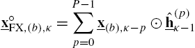
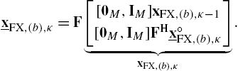
Filtered-X Adaptation of Preprocessors of Partitioned-Block CMs In the following, consider the structure of Fig. 4.4B as a single-tap CGM, for which DFT-domain branch signal vectors can be computed according to Eq. (4.23). Based on that, preprocessed DFT-domain input signal vectors can be determined by
and the DFT-domain FX signal vectors ![]() (see Fig. 4.5 illustrating the FX signals) can be computed by partitioned convolution in a two-step procedure as
(see Fig. 4.5 illustrating the FX signals) can be computed by partitioned convolution in a two-step procedure as
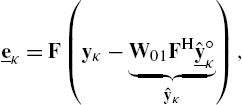
With the introduced signals, the adaptive filter's output can alternatively be determined by one of the two equations
where Eq. (4.33) corresponds to block processing with the signal flow in Fig. 4.4B and Eq. (4.34) corresponds to the signal flow in Fig. 4.5. For time-invariant systems, Eqs. (4.33) and (4.34) are identical. This allows one to compute the error signal vector ![]() and its DFT
and its DFT
both of which will be used for NLMS-type adaptation of the parameters. Analogously to Section 4.3.1.2, a PB-FNLMS adaptation of ![]() can be expressed as
can be expressed as
where ![]() is the normalized preprocessed input signal vector computed analogously to Eqs. (4.26) and (4.27) (containing the adaptation step size) and where Eq. (4.36) and Eq. (4.37) correspond to the unconstrained and the constrained update, respectively.
is the normalized preprocessed input signal vector computed analogously to Eqs. (4.26) and (4.27) (containing the adaptation step size) and where Eq. (4.36) and Eq. (4.37) correspond to the unconstrained and the constrained update, respectively.
Similar to [24], the weights ![]() are estimated by an NLMS algorithm employing the FX signals as
are estimated by an NLMS algorithm employing the FX signals as
with the adaptation step size ![]() and
and
For the more general case where a partitioned-block CGM with ![]() partitions
partitions ![]() replaces the preprocessor with weights
replaces the preprocessor with weights ![]() , all linear combinations with the weights, like in Eq. (4.30), have to be replaced by actual partitioned convolutions and PB-FNLMS updates can be computed for the preprocessor according to
, all linear combinations with the weights, like in Eq. (4.30), have to be replaced by actual partitioned convolutions and PB-FNLMS updates can be computed for the preprocessor according to
and
with the normalized DFT-domain FX branch signal vectors ![]() determined from the FX branch signals
determined from the FX branch signals ![]() analogously to Eqs. (4.26) and (4.27). This corresponds to a generalization of [37] from time-domain power filter preprocessor adaptation to PB-FNLMS adaptation of general CGM preprocessors.
analogously to Eqs. (4.26) and (4.27). This corresponds to a generalization of [37] from time-domain power filter preprocessor adaptation to PB-FNLMS adaptation of general CGM preprocessors.
Thereby, the adaptation of bilinear CMs has been decomposed into two ordinary PB-FNLMS system identification tasks, plus the additional prefiltering operations generating the FX branch signals. All these components can be implemented efficiently using partitioned-block convolution techniques.
An Adaptation Tailored to Single-Tap CGM Preprocessors
In the following, the implications of a parametric preprocessor according to Eq. (4.30) (a single-tap CGM preprocessor, cf. Fig. 4.4B) will be considered in detail. Interestingly, Eq. (4.34) does not introduce cyclic convolution artifacts into ![]() for single-tap filters
for single-tap filters ![]() . Consequently, the cyclic convolution artifacts present in
. Consequently, the cyclic convolution artifacts present in ![]() do not spread by filtering with the weights, allowing to compute the output estimate
do not spread by filtering with the weights, allowing to compute the output estimate

without Eq. (4.32). Furthermore, the zeros in the vector ![]() and the unitarity of the DFT imply
and the unitarity of the DFT imply
Further identifying
as a reasonable approximation of the branch signal energy within a frame allows one to compute the weights according to
without Eq. (4.32) as well. Thus, Eq. (4.32) does not need to be evaluated at all, which allows saving 2B DFTs of length N.
The remaining DFTs and IDFTs are ![]() transforms for computing DFT-domain branch signals prior to Eq. (4.31), the output estimate in Eq. (4.34), and the DFT-domain error signal in Eq. (4.35), as well as 2P DFTs for a constrained update of the partitioned linear subsystem in Eq. (4.37). The computational effort for non-DFT operations has a component growing proportional to
transforms for computing DFT-domain branch signals prior to Eq. (4.31), the output estimate in Eq. (4.34), and the DFT-domain error signal in Eq. (4.35), as well as 2P DFTs for a constrained update of the partitioned linear subsystem in Eq. (4.37). The computational effort for non-DFT operations has a component growing proportional to ![]() due to Eq. (4.31). However, as the effort for a length-N DFT is typically much higher than the effort for a vector multiplication in Eq. (4.31), the number of DFTs may serve as a first indicator of the computational complexity. Thus, the relative computational complexity
due to Eq. (4.31). However, as the effort for a length-N DFT is typically much higher than the effort for a vector multiplication in Eq. (4.31), the number of DFTs may serve as a first indicator of the computational complexity. Thus, the relative computational complexity ![]() of an FX CM and a full-length CGM can be approximated by
of an FX CM and a full-length CGM can be approximated by
which is the ratio of the numbers of involved DFTs plus an overhead ε representing the number of operations which are not DFTs and grow with ![]() in both the FX-CM and the CGM (filtering and filter coefficient updates). To give an example,
in both the FX-CM and the CGM (filtering and filter coefficient updates). To give an example, ![]() and
and ![]() leads to
leads to ![]() and suggests that the CM can be identified with about one-third of the effort of a CGM of the same length.
and suggests that the CM can be identified with about one-third of the effort of a CGM of the same length.
4.3.3 Summary of Algorithms
The main algorithms presented in Section 4.3 are summarized in tabular form to support an implementation in practice. The most basic algorithm is the time-domain NLMS algorithm summarized in Table 4.1. The operations listed therein have to be evaluated at each sample index n. For processing an entire block of M subsequent samples, as in block- and frequency-domain processing, all equations in Table 4.1 have to be evaluated sample by sample for each of the block's samples—M times in total. For PB-FNLMS adaptation, the operations for processing a block of M samples are summarized in Table 4.2. The operations listed therein have to be executed for each signal frame κ (once every M samples). In the same way, the operations required for FX adaptation of a bilinear CM with a single-tap CGM as nonlinear preprocessor are listed in Table 4.3.
Table 4.1
Summary of operations of a time-domain NLMS algorithm for CGMs as executed for each sampling instant n
| computed quantity | computation formula | equation no. | |
|---|---|---|---|
| branch signals |
|
∀b | Eq. (4.11) |
| time-reversed branch signal vectors |
|
∀b | – |
| output signal |
|
Eq. (4.12) | |
| error signal |
|
Eq. (4.13) | |
| frame energy |
|
∀b | Eq. (4.15) |
| filter coefficients |
|
∀b | Eq. (4.14) |

Table 4.2
Summary of operations of a PB-FNLMS algorithm for CGMs as executed for each frame κ
| computed quantity | computation formula | equation no. | |
|---|---|---|---|
| branch signals |
|
∀b | Eq. (4.22) |
| ∼ in DFT domain |
|
∀b | Eq. (4.23) |
| DFT-domain output estimate with cyclic convolution artifacts |
|
Eq. (4.24) | |
| DFT-domain error signal |
|
Eq. (4.25) | |
| branch PSDs |

|
∀b | Eq. (4.26) |
| normalized branch signals |
|
∀b | Eq. (4.27) |
| updated filters |
|
∀b,p | Eq. (4.28) |
| constrained update |
|
∀b,p | Eq. (4.29) |
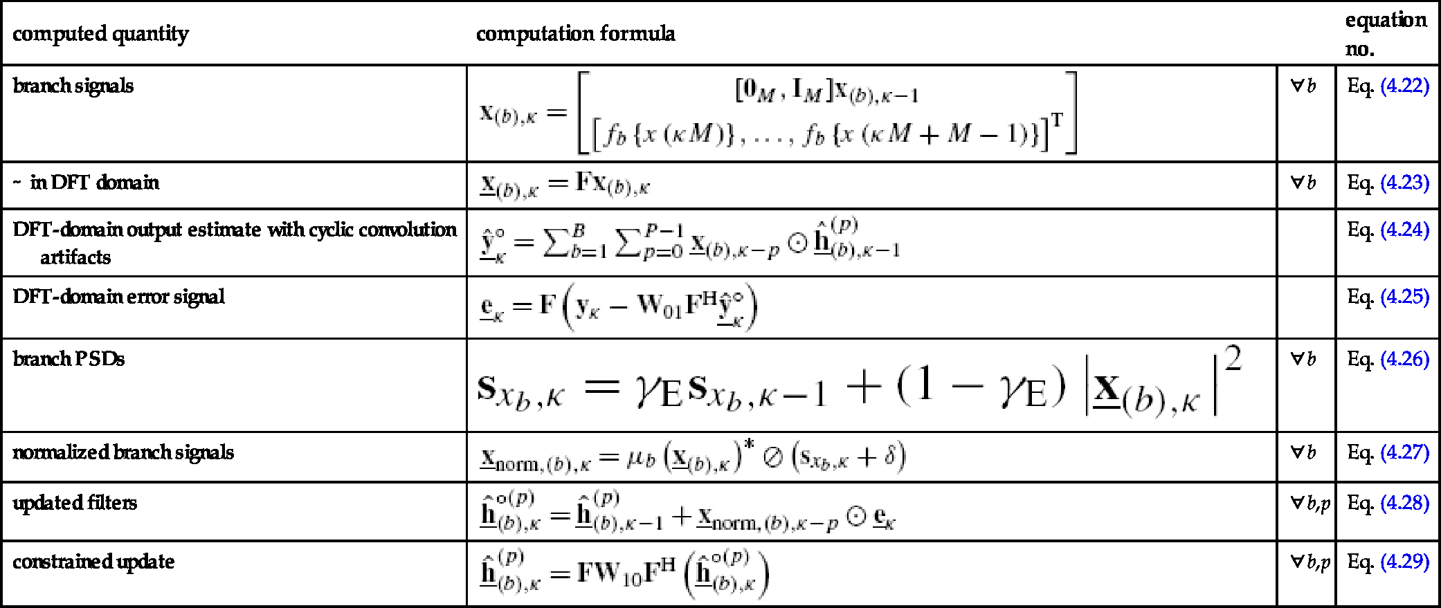
Table 4.3
Summary of operations of an FX algorithm tailored to the adaptation of bilinear CMs with single-tap CGM preprocessors as executed for each frame κ
| computed quantity | computation formula | equation no. | |
|---|---|---|---|
| branch signals |
|
∀b | Eq. (4.22) |
| ∼ to DFT domain |
|
∀b | Eq. (4.23) |
| DFT-domain preprocessed signal |
|
Eq. (4.30) | |
| DFT-domain FX branch signals with cyclic convolution artifacts |
|
∀b,p | Eq. (4.31) |
| output signal |
|
Eq. (4.33) | |
| error signal |
|
– | |
| ∼ to DFT domain |
|
Eq. (4.35) | |
| preprocessed signal PSD |
|
– | |
| normalized input |
|
– | |
| updated filters | ∀p | Eq. (4.40) | |
| constrained update |  , , |
∀p | Eq. (4.41) |
| FX energies |
|
∀b > 1 | Eq. (4.45) |
| weight update |
|
∀b > 1 | Eq. (4.46) |

These algorithms will be employed as building blocks of the computationally very efficient SA filters in the following section, Section 4.4. Therein, the aforementioned basic algorithms will only be referenced without repeating all equations.
4.4 Significance-Aware Filtering
In [28], the concept of SA filtering has been introduced, in order to estimate the parameters of nonlinear CMs by decomposing the adaptation process in a divide-and-conquer manner into synergetic adaptive subsystems [28,30–32] which are LIP. Thereby, the estimation of the nonlinearity is separated from the estimation of a possibly long linear subsystem, as it would be characteristic for acoustic echo paths. As a consequence, the nonlinearity can be estimated computationally efficiently by nonlinear models with a very low number of parameters.
In the following, two different SA decompositions will be introduced in Section 4.4.1 and employed for the Serial SA CMs (SSA-CMs) in Section 4.4.2 (a generalization of the Equalization-based SA (ESA)-HM from [32]), the Parallel SA CGMs (PSA-CGMs) in Section 4.4.3 (a generalization of the SA-HGM from [32]) and a novel Parallel SA Filtered-X (PSAFX) algorithm in Section 4.4.4.
4.4.1 Significance-Aware Decompositions of LIP Nonlinear Systems
In [32], two different SA decompositions have been employed, which will be denoted Serial SA (SSA) decomposition (employed for ESA filtering in [32]) and Parallel SA (PSA) decomposition (employed for so-called “classical” SA filtering in [32]). Both decompositions allow for the estimation of the nonlinearity with a low-complexity nonlinear adaptive filter, as will be explained in the following.
Serial Significance-Aware Decomposition
The SSA decomposition is depicted schematically in Fig. 4.6, where the unknown system is cascaded with an equalizer filter ![]() . The overall response of this serial connection will ideally be a (delayed) version of the nonlinear preprocessor
. The overall response of this serial connection will ideally be a (delayed) version of the nonlinear preprocessor ![]() . Thus, an estimate for the physically inaccessible intermediate signal
. Thus, an estimate for the physically inaccessible intermediate signal ![]() is obtained, which allows one to estimate the nonlinearity directly from this decomposition efficiently by a nonlinear model with a short temporal support. An adaptive system using this decomposition will be specified in Section 4.4.2.
is obtained, which allows one to estimate the nonlinearity directly from this decomposition efficiently by a nonlinear model with a short temporal support. An adaptive system using this decomposition will be specified in Section 4.4.2.
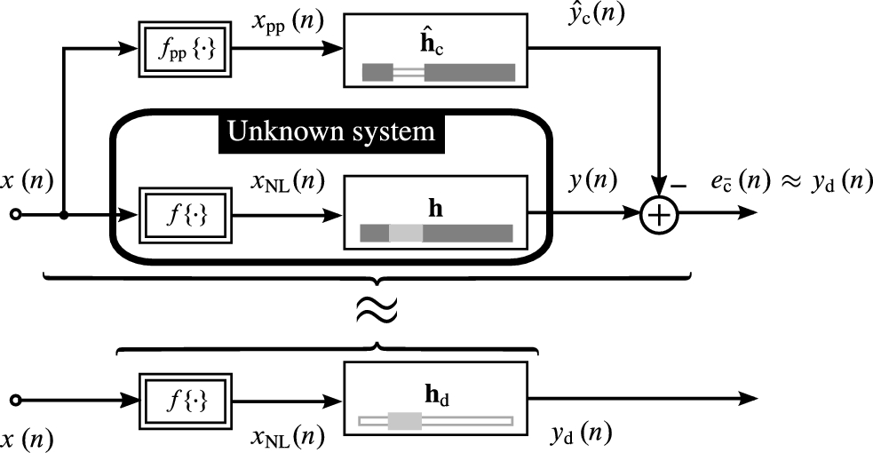
Parallel Significance-Aware Decomposition
The PSA decomposition is illustrated in Fig. 4.7. The LIP property of a nonlinear CM is employed to decompose its IR vector into a dominant region ![]() (light gray), describing, e.g., direct-path propagation, and a complementary region
(light gray), describing, e.g., direct-path propagation, and a complementary region ![]() (dark gray). Augmenting the unknown system with a parallel system modeling the complementary-region output signal component
(dark gray). Augmenting the unknown system with a parallel system modeling the complementary-region output signal component ![]() allows one to compute the dominant-region output component
allows one to compute the dominant-region output component ![]() . As
. As ![]() ,
, ![]() ,
, ![]() , and thereby
, and thereby ![]() are not known during system identification, they have to be replaced by estimates
are not known during system identification, they have to be replaced by estimates ![]() ,
, ![]() ,
, ![]() and
and ![]() in practice, as depicted in the upper part of Fig. 4.7. Still, the output of the parallel arrangement yields an estimate
in practice, as depicted in the upper part of Fig. 4.7. Still, the output of the parallel arrangement yields an estimate ![]() of the dominant-region component of the unknown system (bottom of Fig. 4.7). As the dominant-region component of the system describes the transmission of a significant amount of energy, a nonlinear dominant-region model can be estimated at a high Signal to Noise Ratio (SNR) and will suffer much less from gradient noise than a reverberation tail model. Adaptive systems using this decomposition will be specified in Sections 4.4.3 and 4.4.4.
of the dominant-region component of the unknown system (bottom of Fig. 4.7). As the dominant-region component of the system describes the transmission of a significant amount of energy, a nonlinear dominant-region model can be estimated at a high Signal to Noise Ratio (SNR) and will suffer much less from gradient noise than a reverberation tail model. Adaptive systems using this decomposition will be specified in Sections 4.4.3 and 4.4.4.
Estimating a Preprocessor System From a CGM
Another key component for the SA models described in Sections 4.4.2 and 4.4.3 below is the possibility to extract a CM's preprocessor from an identified CGM-structured estimate of the CM system. To this end, assume that the CM's nonlinearity can be expressed as weighted sum of the CGM's branch nonlinearities ![]() , resulting in an expression identical to Eq. (4.8). The CM's linear subsystem will be denoted h. Then, the CM can be expressed as CGM with linear subsystems
, resulting in an expression identical to Eq. (4.8). The CM's linear subsystem will be denoted h. Then, the CM can be expressed as CGM with linear subsystems ![]() . In practice, an identified CGM can only provide noisy estimates
. In practice, an identified CGM can only provide noisy estimates
where ![]() is the coefficient error vector. As shown in [28], a least squares estimate for
is the coefficient error vector. As shown in [28], a least squares estimate for ![]() can be obtained by
can be obtained by
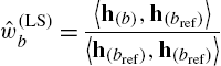
w.r.t. a reference branch ![]() , for which
, for which ![]() . Note that
. Note that ![]() is not a model restriction—it simply removes the scaling ambiguity inherent to the cascade model by shifting the actual
is not a model restriction—it simply removes the scaling ambiguity inherent to the cascade model by shifting the actual ![]() as gain factor into the estimate
as gain factor into the estimate ![]() to be identified after the preprocessor. Without loss of generality,
to be identified after the preprocessor. Without loss of generality, ![]() and
and ![]() will be assumed from now on. A preprocessor with
will be assumed from now on. A preprocessor with ![]() will be referred to as linearly configured preprocessor.
will be referred to as linearly configured preprocessor.
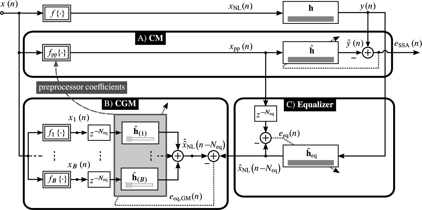
4.4.2 Serial Significance-Aware Cascade Models
SSA-CMs employ the SSA decomposition from Fig. 4.6 and generalize the Serial SA HMs (SSA-HMs) from [32] by allowing branch nonlinearities with memory. The structure of an SSA-CM is depicted in Fig. 4.8. Initially, the preprocessor in Block A in Fig. 4.8, providing the signal ![]() , is configured to be linear. After this initialization, all subsystems in Fig. 4.8 are adapted in parallel. In Block C in Fig. 4.8, an adaptive linear equalizer implements the SSA decomposition. The equalizer filters the unknown system's output
, is configured to be linear. After this initialization, all subsystems in Fig. 4.8 are adapted in parallel. In Block C in Fig. 4.8, an adaptive linear equalizer implements the SSA decomposition. The equalizer filters the unknown system's output ![]() to produce an estimate
to produce an estimate ![]() of the delayed nonlinearly distorted input signal. For adaptation,
of the delayed nonlinearly distorted input signal. For adaptation, ![]() is matched to
is matched to ![]() .5 Ideally,
.5 Ideally, ![]() and
and ![]() are time-aligned as well and related by
are time-aligned as well and related by ![]() (cf. Fig. 4.6). Thus, the nonlinear relationship between
(cf. Fig. 4.6). Thus, the nonlinear relationship between ![]() and
and ![]() can be estimated by a very short adaptive CGM of
can be estimated by a very short adaptive CGM of ![]() taps in Block B in Fig. 4.8. Although
taps in Block B in Fig. 4.8. Although ![]() would be sufficient in the case of a perfect equalization of h, a very small
would be sufficient in the case of a perfect equalization of h, a very small ![]() of about
of about ![]() is reasonable in practice due to the adaptive, imperfect equalizer. Between Blocks B and A in Fig. 4.8, the identified CGM and Eq. (4.49) are employed to estimate the coefficients of a preprocessor which combines the CGM's branch signals according to Eq. (4.8). Analogously to [32], the preprocessor coefficients
is reasonable in practice due to the adaptive, imperfect equalizer. Between Blocks B and A in Fig. 4.8, the identified CGM and Eq. (4.49) are employed to estimate the coefficients of a preprocessor which combines the CGM's branch signals according to Eq. (4.8). Analogously to [32], the preprocessor coefficients ![]() are estimated on a frame-wise basis as
are estimated on a frame-wise basis as
where ![]() , is a recursive-smoothing constant (
, is a recursive-smoothing constant (![]() will be used by default for the simulations in Section 4.5) and
will be used by default for the simulations in Section 4.5) and ![]() is computed according to Eq. (4.49) from the instantaneous estimates of the branch signal vectors of the CGM of Block B. The preprocessor with weights
is computed according to Eq. (4.49) from the instantaneous estimates of the branch signal vectors of the CGM of Block B. The preprocessor with weights ![]() is used in a CM with an adaptive linear subsystem to model the entire unknown system (Block A in Fig. 4.8).
is used in a CM with an adaptive linear subsystem to model the entire unknown system (Block A in Fig. 4.8).
 of the nonlinearly distorted input signal is obtained in Block C by equalizing the system output signal with a linear equalizer, which allows in Block B to assess the nonlinear distortions by a very short CGM, which in turn is employed for estimating the parameters of the nonlinear preprocessor
  of Block A.
The SSA-CM structure according to Fig. 4.8 is efficient, because it requires only two adaptive linear filters with long temporal support (in Blocks A and C), both of which will be assumed to have length L, and a CGM with a very low number of taps ![]() . A number of
. A number of ![]() taps will be assumed by default in the following. The long adaptive filters can be realized efficiently using a PB-FNLMS according to Section 4.3.1.2 in a block processing scheme and the CGM can be implemented due to its short length at very low computational effort by a time-domain NLMS according to Section 4.3.1.1. Hence, the computational effort for an SSA-CM is roughly twice as high as that for a linear filter. The relative complexity compared with a CGM,
taps will be assumed by default in the following. The long adaptive filters can be realized efficiently using a PB-FNLMS according to Section 4.3.1.2 in a block processing scheme and the CGM can be implemented due to its short length at very low computational effort by a time-domain NLMS according to Section 4.3.1.1. Hence, the computational effort for an SSA-CM is roughly twice as high as that for a linear filter. The relative complexity compared with a CGM, ![]() , is about
, is about
where the contribution of the length-![]() CGM has been disregarded. For
CGM has been disregarded. For ![]() branches and
branches and ![]() partitions, this leads to
partitions, this leads to ![]() .
.
4.4.3 Parallel Significance-Aware Cascade Group Models
PSA-CGMs generalize the SA-HGMs from [28,31] by allowing branch nonlinearities with memory and are structurally identical otherwise. The structure of such a PSA-CGM is depicted in Fig. 4.9. For an explanation of the general concept, assume that the temporal support of the unknown system's dominant region (cf. Fig. 4.7) is known. In this case, all adaptive systems in Fig. 4.9 can be adapted simultaneously.
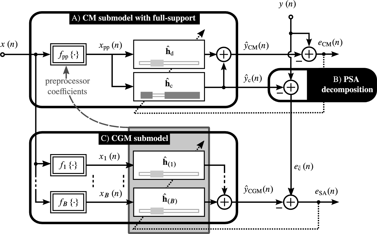
Block A of Fig. 4.9 contains a CM with adaptive linear subsystem (minimizing the error signal ![]() ). The nonlinear parametric preprocessor
). The nonlinear parametric preprocessor ![]() is initially configured as linear function and is refined separately from the IR. The CM's IR estimate is partitioned into a dominant region
is initially configured as linear function and is refined separately from the IR. The CM's IR estimate is partitioned into a dominant region ![]() (upper branch in Block A) and a complementary region
(upper branch in Block A) and a complementary region ![]() (lower branch in Block A). This allows one to apply the PSA decomposition (cf. Fig. 4.7) to the unknown system in Block B in Fig. 4.9: subtracting the complementary-region estimate
(lower branch in Block A). This allows one to apply the PSA decomposition (cf. Fig. 4.7) to the unknown system in Block B in Fig. 4.9: subtracting the complementary-region estimate ![]() from the unknown system's output
from the unknown system's output ![]() results in the dominant-region dominated error signal
results in the dominant-region dominated error signal ![]() . This enables in Block C of Fig. 4.9 the identification of the unknown system's dominant region alone by a CGM with short temporal support (as short as
. This enables in Block C of Fig. 4.9 the identification of the unknown system's dominant region alone by a CGM with short temporal support (as short as ![]() ). The CGM's IRs
). The CGM's IRs ![]() allow one to extract the preprocessor coefficients for the CM in Block A of Fig. 4.9 analogously to Section 4.4.2. It is worth noting that a PSA-CGM offers two different error signals:
allow one to extract the preprocessor coefficients for the CM in Block A of Fig. 4.9 analogously to Section 4.4.2. It is worth noting that a PSA-CGM offers two different error signals: ![]() , resulting from a CM output signal estimate
, resulting from a CM output signal estimate ![]() , and
, and ![]() , resulting from
, resulting from ![]() (not shown in Fig. 4.9). The estimate
(not shown in Fig. 4.9). The estimate ![]() is obtained with a CGM as dominant-path model and represents a more general model than the CM in Block A of Fig. 4.9. If the unknown system has a CM structure,
is obtained with a CGM as dominant-path model and represents a more general model than the CM in Block A of Fig. 4.9. If the unknown system has a CM structure, ![]() may be slightly more accurate than
may be slightly more accurate than ![]() , because the CGM has more degrees of freedom than necessary and is more affected by gradient noise. If the unknown system is more complex than a CM, the additional degrees of freedom of the CGM may render
, because the CGM has more degrees of freedom than necessary and is more affected by gradient noise. If the unknown system is more complex than a CM, the additional degrees of freedom of the CGM may render ![]() more accurate. For this reason, the PSA-CGM will appear in the evaluation in Section 4.5 twice.
more accurate. For this reason, the PSA-CGM will appear in the evaluation in Section 4.5 twice.
For a highly efficient low-delay realization of the PSA-CGM, a PB-FNLMS implementation has been proposed in [31]. This method identifies partitions ![]() of the linear subsystem of the CM in Block A of Fig. 4.9 by a PB-FNLMS (Section 4.3.1.2,
of the linear subsystem of the CM in Block A of Fig. 4.9 by a PB-FNLMS (Section 4.3.1.2, ![]() branches and
branches and ![]() partitions). Employing this partitioning, the dominant region is modeled by a single partition
partitions). Employing this partitioning, the dominant region is modeled by a single partition ![]() with index
with index ![]() and the complementary region is composed of all other partitions, where
and the complementary region is composed of all other partitions, where ![]() . As a consequence, the nonlinear dominant-region model of Block C in Fig. 4.9 is a single-partition CGM and adapted according to Section 4.3.1.2 (
. As a consequence, the nonlinear dominant-region model of Block C in Fig. 4.9 is a single-partition CGM and adapted according to Section 4.3.1.2 (![]() branches and
branches and ![]() partition).
partition).
If the temporal support of the dominant region is unknown, only ![]() are adapted in an initial convergence phase. Afterwards, the fixed-length partitions
are adapted in an initial convergence phase. Afterwards, the fixed-length partitions ![]() allow one to detect a dominant partition
allow one to detect a dominant partition ![]() as the partition with maximum energy. Compared to a full-length CGM with P partitions in each branch, the relative computational complexity
as the partition with maximum energy. Compared to a full-length CGM with P partitions in each branch, the relative computational complexity ![]() of a PSA-CGM is approximately
of a PSA-CGM is approximately
Obviously, the PSA-CGM is very efficient for large P and B. Without block partitioning (P=1), however, the described PSA-CGM does not provide any advantage. To give an example, ![]() and
and ![]() results in
results in ![]() .
.
4.4.4 Parallel Significance-Aware Filtered-X Adaptation
In this section, a novel SA filtering concept will be introduced. This concept exploits the PSA decomposition for the direct FX adaptation of bilinear CMs from Section 4.2.3 (see Fig. 4.7) and will be denoted Parallel SA Filtered-X CM (PSAFX-CM). The block diagram of the PSAFX-CM matches the block diagram of the PSA-CGM in Fig. 4.9, except for Block C. Like for the PSA-CGM, a CM with an adaptive linear subsystem (Block A in Fig. 4.9) enables a PSA decomposition (Block B in Fig. 4.9); in an initialization phase, the CM preprocessor is configured as linear function and only the IR is adapted. Afterwards, the CM's IR is split into a dominant and a complementary region. The complementary-region submodel is used (as in Block B in Fig. 4.9) to compute an error signal ![]() . This error signal mainly contains components
. This error signal mainly contains components ![]() , which are caused by the unknown system's dominant region (see also Fig. 4.7).
, which are caused by the unknown system's dominant region (see also Fig. 4.7).
As an alternative to the PSA-CGM, the novel PSAFX-CM implements the adaptive nonlinear model for the dominant region (Block C) according to Fig. 4.10. Therein, the PSAFX-CM employs a dominant-region CM with ![]() from Block A in Fig. 4.9 and FX-adapted preprocessor weights
from Block A in Fig. 4.9 and FX-adapted preprocessor weights ![]() . As it is characteristic for SA filtering, the preprocessor determined for the dominant region is then applied in the CM with the full-length adaptive linear subsystem (Block A in Fig. 4.9). Note that the complementary-region CM from Block A in Fig. 4.9 and the dominant-region CM from Fig. 4.10 seamlessly combine to the overall CM of Block A in Fig. 4.9 again. This implies
. As it is characteristic for SA filtering, the preprocessor determined for the dominant region is then applied in the CM with the full-length adaptive linear subsystem (Block A in Fig. 4.9). Note that the complementary-region CM from Block A in Fig. 4.9 and the dominant-region CM from Fig. 4.10 seamlessly combine to the overall CM of Block A in Fig. 4.9 again. This implies ![]() . Thus, the only difference from an ordinary FX implementation is that the FX branch signals are generated with the most significant fragment of
. Thus, the only difference from an ordinary FX implementation is that the FX branch signals are generated with the most significant fragment of ![]() .
.

 of a dominant-region CM are adapted using an FX algorithm with
  from Block A in Fig. 4.9 as linear subsystem of the CM and with
  from the PSA decomposition in Block B in Fig. 4.9 as target signal.
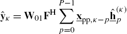
Pursuing a PB-FNLMS implementation as in Section 4.3.2, the adaptation procedures are identical up to Eq. (4.31), and Eq. (4.31) simplifies to the single partition
and is therefore independent of the length of the actually modeled unknown system. Unlike for the FX algorithm of Section 4.3.2, the filtering effort for generating the FX signals is not proportional to ![]() anymore, but only to B. As a consequence, the relative complexity
anymore, but only to B. As a consequence, the relative complexity ![]() of a PSAFX-CM w.r.t. a full-length CGM can be estimated by the number of DFTs and yields
of a PSAFX-CM w.r.t. a full-length CGM can be estimated by the number of DFTs and yields
The overhead ε from Eq. (4.47), caused by non-DFT operations with a complexity proportional to ![]() , does not appear in Eq. (4.52) as the actual filtering effort is reduced to a complexity proportional to B only. To give an example,
, does not appear in Eq. (4.52) as the actual filtering effort is reduced to a complexity proportional to B only. To give an example, ![]() and
and ![]() leads to
leads to ![]() and thereby indicates a computationally very inexpensive nonlinear model, which is even less complex than the other SA filters.
and thereby indicates a computationally very inexpensive nonlinear model, which is even less complex than the other SA filters.
As for the other SA models in Sections 4.4.2 and 4.4.3, the nonlinear system identification has been split into synergetic subsystems, where the first models the possibly long memory of the linear subsystem (Block A in Fig. 4.9) and the second estimates the nonlinearities without modeling the possibly long memory of the system (Fig. 4.10).
4.5 Experiments and Evaluation
In this section, the adaptive LIP nonlinear filters from Sections 4.3 and 4.4 will be evaluated exemplarily for the challenging application of AEC (cf. Section 4.1). To this end, the evaluation method will be introduced in Section 4.5.1 and the experiments will be presented and discussed in Section 4.5.2.
Note that, in principle, the presented methods can also be employed for many applications aside from AEC. In particular, the identification of the path between the discrete-time loudspeaker signal and a recording of the radiated sound can also be the first step towards a loudspeaker linearization [7–9] or nonlinear active noise control [68,53]. Furthermore, the presented algorithms can enable the identification of nonlinear analog signal processors (e.g., guitar amplifier and effect processor devices [69,70]) to emulate the identified processors in digital hardware afterwards. Moreover, the joints of robots can be modeled as HMs as well [71] and may be identified with the methods of Section 4.3. Lifting the latter example to a broad industrial scope, the adaptive algorithms presented in this chapter may be employed for digital twin modeling (also termed cybertwin) of nonlinear mechanical, electrical, acoustical or chemical systems in digitalized production plants for Industry 4.0 [72]—as long as the underlying nonlinear systems can be described well by CMs. However, the longer the linear subsystem of an HM or CM is, the more computational benefit can be expected by SA modeling. In case of short linear subsystems, block partitioning and frequency-domain processing may be unnecessary and time-domain adaptation of all involved adaptive linear filters should be pursued (see [28] for a time-domain SA filter).
4.5.1 Evaluation Metrics
For system identification, normalized misalignment [24] and projection misalignment measures [73] evaluate how well particular components of a parametrized system are identified. However, these measures require the exact knowledge of the true system parameters—knowledge which is typically not available for actual physical systems to be identified. In this case, signal-based measures have to be adopted. In particular, the modeling accuracy can be measured by the ratio of the variance of the unknown system's output ![]() and of the residual error
and of the residual error ![]() .
.
For the special system identification case of AEC, where the primary objective is the removal of the loudspeaker signal components (echoes) from the microphone signal, this ratio of variances is widely known as Echo-Return Loss Enhancement (ERLE) and is usually considered in the logarithmic domain according to
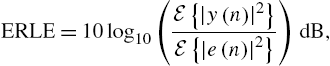
assuming noise-free “single talk” situations (no speaker or noise on the near end, only an echo signal). A higher ERLE measure corresponds to a better performance of the AEC system [74]. When estimating the ERLE in short time frames employing the instantaneous energies of ![]() and
and ![]() and continuously adapting the model, even severe overadaptation to the particular signal may remain unnoticed and be misinterpreted as accurate system identification because of the high ERLE values. To minimize this undesired effect, filtering a long interval of speech with frozen filter coefficients after convergence is possible. The resulting ERLE can be used as system identification performance measure. An ERLE computed in this way also evaluates the primary use case of an AEC system, as it captures the amount of echo reduction in the presence of near-end speech (double talk), when the adaptive filters cannot be adapted and the recording cannot be muted (no half-duplex but full-duplex communication) [74]. The ERLE measure for frozen filter coefficients will be employed in the following to evaluate and compare the adaptive filtering algorithms described in Sections 4.3 and 4.4.
and continuously adapting the model, even severe overadaptation to the particular signal may remain unnoticed and be misinterpreted as accurate system identification because of the high ERLE values. To minimize this undesired effect, filtering a long interval of speech with frozen filter coefficients after convergence is possible. The resulting ERLE can be used as system identification performance measure. An ERLE computed in this way also evaluates the primary use case of an AEC system, as it captures the amount of echo reduction in the presence of near-end speech (double talk), when the adaptive filters cannot be adapted and the recording cannot be muted (no half-duplex but full-duplex communication) [74]. The ERLE measure for frozen filter coefficients will be employed in the following to evaluate and compare the adaptive filtering algorithms described in Sections 4.3 and 4.4.
4.5.2 Experiments
In this section, the ERLE performance of the adaptive algorithms from Sections 4.3 and 4.4 will be compared in AEC experiments. To this end, the nonlinear echo paths of different devices will be considered. Device 1 is a smartphone in hands-free mode, Device 2 is a low-quality electrodynamic loudspeaker and Device 3 is a cellphone manufactured in the year 2000. About ![]() of speech (both male and female speech) have been played back at relatively high volumes of about
of speech (both male and female speech) have been played back at relatively high volumes of about ![]() at
at ![]() distance and recorded with the playback device itself for Device 1 and with a high-quality measurement microphone at
distance and recorded with the playback device itself for Device 1 and with a high-quality measurement microphone at ![]() distance for Devices 2 and 3. All AEC experiments were conducted at a sampling rate of
distance for Devices 2 and 3. All AEC experiments were conducted at a sampling rate of ![]() and in three acoustic environments, denoted Scenarios 1, 2 and 3. The actual recordings were performed under low-reverberation conditions, which corresponds to Scenario 1. The data for Scenarios 2 and 3 are synthesized from the low-reverberation recordings by convolving the recordings with measured acoustic IRs from real lab environments with reverberation times of
and in three acoustic environments, denoted Scenarios 1, 2 and 3. The actual recordings were performed under low-reverberation conditions, which corresponds to Scenario 1. The data for Scenarios 2 and 3 are synthesized from the low-reverberation recordings by convolving the recordings with measured acoustic IRs from real lab environments with reverberation times of ![]() and
and ![]() , respectively. The adaptive filters employed for the identification of the acoustic echo path will be realized, as specified earlier in this chapter, as partitioned-block adaptive filters in the frequency domain. For all scenarios and devices, a linear filter (Section 4.3.1.2 with
, respectively. The adaptive filters employed for the identification of the acoustic echo path will be realized, as specified earlier in this chapter, as partitioned-block adaptive filters in the frequency domain. For all scenarios and devices, a linear filter (Section 4.3.1.2 with ![]() branches and
branches and ![]() ), a CM with FX adaptation tailored to memoryless preprocessors (Section 4.3.2), a CM with PSAFX adaptation (Section 4.4.4), a PSA-CGM (Section 4.4.3), an SSA-CM (Section 4.4.2) and a CGM with full temporal support (Section 4.3.1.2) will be compared. All adaptive filters are identically parametrized by step sizes of
), a CM with FX adaptation tailored to memoryless preprocessors (Section 4.3.2), a CM with PSAFX adaptation (Section 4.4.4), a PSA-CGM (Section 4.4.3), an SSA-CM (Section 4.4.2) and a CGM with full temporal support (Section 4.3.1.2) will be compared. All adaptive filters are identically parametrized by step sizes of ![]() , block processing is done at a frame shift of
, block processing is done at a frame shift of ![]() samples and a frame size of
samples and a frame size of ![]() and the block-partitioned filters consist of
and the block-partitioned filters consist of ![]() partitions of length M. Furthermore, the equalizer delay for the SSA-CM is chosen as
partitions of length M. Furthermore, the equalizer delay for the SSA-CM is chosen as ![]() samples. All nonlinear models have
samples. All nonlinear models have ![]() branches and preprocessor coefficients, respectively, and employ odd-order Legendre polynomials of orders 1 to 9 as branch nonlinearities
branches and preprocessor coefficients, respectively, and employ odd-order Legendre polynomials of orders 1 to 9 as branch nonlinearities ![]() . Thereby, all CGMs are HGMs and all CMs are HMs. The computational complexity of the individual models relative to the complexity of a CGM is listed in Table 4.4. Therein, the first line (“approximate”) corresponds to the relative complexity estimates introduced with the algorithms in Sections 4.3 and 4.4. The second line (“FLOPS”) contains the relative numbers of FLoating Point Operations (FLOPS) of the particular method in comparison to a CGM. To this end, the FLOPS have been determined analogously to [32]. Operations counted as FLOPS are real-valued additions, multiplications and divisions. The complex-valued DFT-domain operations are considered by mapping complex-valued additions, multiplications and divisions to multiple real-valued operations. In particular, a complex-valued addition is counted as 2 real-valued FLOPS, a complex-valued multiplication is counted as 6 real-valued FLOPS and the division of a complex number by a real-valued number is counted as 2 real-valued FLOPS. Accumulating the FLOPS of all equations necessary for processing a signal frame of M samples by a particular filter structure corresponds to the algorithm's number of FLOPS. Normalizing these FLOPS to the FLOPS of a CGM leads to the relative FLOPS in line two of Table 4.4.
. Thereby, all CGMs are HGMs and all CMs are HMs. The computational complexity of the individual models relative to the complexity of a CGM is listed in Table 4.4. Therein, the first line (“approximate”) corresponds to the relative complexity estimates introduced with the algorithms in Sections 4.3 and 4.4. The second line (“FLOPS”) contains the relative numbers of FLoating Point Operations (FLOPS) of the particular method in comparison to a CGM. To this end, the FLOPS have been determined analogously to [32]. Operations counted as FLOPS are real-valued additions, multiplications and divisions. The complex-valued DFT-domain operations are considered by mapping complex-valued additions, multiplications and divisions to multiple real-valued operations. In particular, a complex-valued addition is counted as 2 real-valued FLOPS, a complex-valued multiplication is counted as 6 real-valued FLOPS and the division of a complex number by a real-valued number is counted as 2 real-valued FLOPS. Accumulating the FLOPS of all equations necessary for processing a signal frame of M samples by a particular filter structure corresponds to the algorithm's number of FLOPS. Normalizing these FLOPS to the FLOPS of a CGM leads to the relative FLOPS in line two of Table 4.4.
Table 4.4
Computational complexity of linear and nonlinear models relative to a CGM with B = 5 branches and P = 4 partitions. The approximate values are a summary of the numbers in the individual algorithms' sections, whereas the number of FLOPS are computed analogously to [32] for a frameshift of M = 512
| linear | PSAFX-CM | FX-CM | SSA-CM | PSA-CGM | CGM | |
|---|---|---|---|---|---|---|
| approximate | 0.23 | 0.32 | 0.32 + ε | 0.40 | 0.45 | 1 |
| FLOPs | 0.23 | 0.32 | 0.37 | 0.50 | 0.58 | 1 |

Obviously, the qualitative rating of the different algorithms in Table 4.4 is similar by both complexity estimation methods: the further right an algorithm is in Table 4.4, the more computationally demanding it is.
The ERLE achievable with the different adaptive filter structures with frozen parameters (like during double talk) is listed in Figs. 4.11A to 4.11C for Devices 1 to 3, respectively. Obviously, linear AEC (A in Fig. 4.11) suffers a lot from the severe nonlinearities, leading to ERLE below ![]() under all reverberation conditions and to particularly bad performance under the low-reverberation conditions of Scenario 1. All nonlinear models outperform the linear model for all devices and scenarios. The CGM (G in Fig. 4.11), being the most complex model, shows consistently high performance. However, in particular the PSA-CGM (E and F in Fig. 4.11) approaches or even outperforms the more complex CGM. Especially the PSA-CGM's CM output (E in Fig. 4.11) performs very well. This confirms that the actual acoustic echo paths can be approximated well by CMs. However, the FX adaptation of a CM (C in Fig. 4.11) closely approaches the performance of the CGM only for Device 1. Still, introducing further efficiency into the FX adaptation by a PSA decomposition (B in Fig. 4.11) does not lead to any noticeable disadvantage. The SSA-CM performance (D in Fig. 4.11) resembles the performance of other nonlinear approaches for Device 1, but performs worse for the other devices (while still outperforming the linear filter).
under all reverberation conditions and to particularly bad performance under the low-reverberation conditions of Scenario 1. All nonlinear models outperform the linear model for all devices and scenarios. The CGM (G in Fig. 4.11), being the most complex model, shows consistently high performance. However, in particular the PSA-CGM (E and F in Fig. 4.11) approaches or even outperforms the more complex CGM. Especially the PSA-CGM's CM output (E in Fig. 4.11) performs very well. This confirms that the actual acoustic echo paths can be approximated well by CMs. However, the FX adaptation of a CM (C in Fig. 4.11) closely approaches the performance of the CGM only for Device 1. Still, introducing further efficiency into the FX adaptation by a PSA decomposition (B in Fig. 4.11) does not lead to any noticeable disadvantage. The SSA-CM performance (D in Fig. 4.11) resembles the performance of other nonlinear approaches for Device 1, but performs worse for the other devices (while still outperforming the linear filter).

To sum up, all SA filters successfully alleviate the computational burden for nonlinear AEC. The performance of a general CGM can be reached in the experiments by an efficient PSA-CGM. An even less complex (but also less effective) direct CM adaptation by an FX algorithm can benefit in terms of computational complexity from PSA filtering without losing ERLE performance.
4.6 Outlook on Model Structure Estimation
All methods described in this chapter identify the parameters of nonlinear models adaptively. Yet, the algorithms do not choose an optimum model structure, such as a particular base function set, the order of a polynomial nonlinearity, or the memory length of linear subsystems. However, knowledge about the model structure is highly desirable for two reasons. First, minimizing the number of parameters leads to computational efficiency and second, unnecessarily estimated and redundant parameters introduce gradient noise (estimation errors) and consequently reduce the accuracy of the model.
Both disadvantages can be tackled by employing convex filter combinations [75], as described in Chapter 11. To briefly illustrate this concept for the scope of this chapter, consider two competing models A and B with the respective outputs ![]() and
and ![]() , modeling the same system with output
, modeling the same system with output ![]() . Although modeling the same system, the models A and B are assumed to have a different structure (e.g., memory length of linear subsystems) and consequently different numbers and values of parameters (e.g., filter coefficients of linear subsystems). Convex filter combinations superimpose the outputs
. Although modeling the same system, the models A and B are assumed to have a different structure (e.g., memory length of linear subsystems) and consequently different numbers and values of parameters (e.g., filter coefficients of linear subsystems). Convex filter combinations superimpose the outputs ![]() and
and ![]() according to
according to
where the mixing weight ![]() , is determined adaptively. In practice, this can perform like an adaptive switch indicating the more suitable of the two competing models and thereby the more suitable model structure. Convex combination-based methods for structure estimation can be applied to all kinds of CGMs (e.g., Volterra, Legendre, Chebyshev and Fourier nonlinear filters). As the structure estimation methods are described for the example of Volterra filters in the original publications, the methods will be explained here first for Volterra filters. To this end, consider Volterra filters, which consist of kernels of orders
, is determined adaptively. In practice, this can perform like an adaptive switch indicating the more suitable of the two competing models and thereby the more suitable model structure. Convex combination-based methods for structure estimation can be applied to all kinds of CGMs (e.g., Volterra, Legendre, Chebyshev and Fourier nonlinear filters). As the structure estimation methods are described for the example of Volterra filters in the original publications, the methods will be explained here first for Volterra filters. To this end, consider Volterra filters, which consist of kernels of orders ![]() , with maximum order O. Each kernel consists of diagonals with maximum relative time lags
, with maximum order O. Each kernel consists of diagonals with maximum relative time lags ![]() in the branch nonlinearities of the oth kernel (
in the branch nonlinearities of the oth kernel (![]() is also known as diagonal radius) and has linear subsystems of length
is also known as diagonal radius) and has linear subsystems of length ![]() in kernel o. As O,
in kernel o. As O, ![]() and
and ![]() determine the model structure, they will be referred to as the structure parameters of the Volterra model. These structure parameters determine which of the filter coefficients of a Volterra filter are modeled in practice.
determine the model structure, they will be referred to as the structure parameters of the Volterra model. These structure parameters determine which of the filter coefficients of a Volterra filter are modeled in practice.
As proposed in [43], an identified model can automatically be trimmed by an additional adaptive structure, where a Volterra kernel is clustered into disjoint groups of diagonals and each group's output signal ![]() , where g is the group index, is replaced by a convex combination of the group's output
, where g is the group index, is replaced by a convex combination of the group's output ![]() with 0 (the result of filtering with an all-zero kernel region). Thereby, irrelevant diagonals, which are dominated by noise and would increase the modeling error, can be trimmed for the final computation of the model output. Thereby, the modeling accuracy is increased at the expense of a slight increase in computational complexity. In this case, the mixing variables of the convex combinations take the role of additional structure parameters. In a similar way, the FLAFs in [48] disable nonlinear model parts as well. Another related approach is the so-called EVOLVE concept [76], which approaches the estimation of a Volterra filter structure in a bottom-up way by starting with a small filter and successively growing the model until the optimal size is reached. Filters which are evolutionary w.r.t. a structure parameter dimension
with 0 (the result of filtering with an all-zero kernel region). Thereby, irrelevant diagonals, which are dominated by noise and would increase the modeling error, can be trimmed for the final computation of the model output. Thereby, the modeling accuracy is increased at the expense of a slight increase in computational complexity. In this case, the mixing variables of the convex combinations take the role of additional structure parameters. In a similar way, the FLAFs in [48] disable nonlinear model parts as well. Another related approach is the so-called EVOLVE concept [76], which approaches the estimation of a Volterra filter structure in a bottom-up way by starting with a small filter and successively growing the model until the optimal size is reached. Filters which are evolutionary w.r.t. a structure parameter dimension ![]() perform a convex combination of a filter with a small model size (a low structure parameter value
perform a convex combination of a filter with a small model size (a low structure parameter value ![]() ) and of a filter with a larger model size (a larger structure parameter value
) and of a filter with a larger model size (a larger structure parameter value ![]() ). In the case of a clear preference of one of both models, both models are grown or shrunk into the preferred direction. Note that, for reasons of efficiency, the larger model can also be “virtualized” by simply augmenting the small model with additional filter coefficients [76,77]. As described in [76], an evolution in
). In the case of a clear preference of one of both models, both models are grown or shrunk into the preferred direction. Note that, for reasons of efficiency, the larger model can also be “virtualized” by simply augmenting the small model with additional filter coefficients [76,77]. As described in [76], an evolution in ![]() and
and ![]() and bypassing kernel orders is possible by cascading multiple convex combinations, each of which decides for the activation of another region of filter taps of the Volterra filter. This concept can, of course, be applied to CGMs with other branch nonlinearities as well: Legendre-based CGMs (cf., [45,46] or Section 4.5.2), where ith powers in the Volterra filters' branch nonlinearities are replaced by ith-order Legendre polynomials, have the same set of structure parameters
and bypassing kernel orders is possible by cascading multiple convex combinations, each of which decides for the activation of another region of filter taps of the Volterra filter. This concept can, of course, be applied to CGMs with other branch nonlinearities as well: Legendre-based CGMs (cf., [45,46] or Section 4.5.2), where ith powers in the Volterra filters' branch nonlinearities are replaced by ith-order Legendre polynomials, have the same set of structure parameters ![]() and can be grown the same way as Volterra filters in an EVOLVE fashion. Also, the model trimming from [43] can directly be applied to such Legendre-based CGMs. As opposed to [43], EVOLVE [76] starts with a low-complexity model and successively grows the model if required. Thereby, not only gradient noise in irrelevant filter coefficients is prevented, but also the computational complexity is only as high as the complexity of the optimum filter structure found by the algorithm, plus some overhead for the virtualized models of increased size.
and can be grown the same way as Volterra filters in an EVOLVE fashion. Also, the model trimming from [43] can directly be applied to such Legendre-based CGMs. As opposed to [43], EVOLVE [76] starts with a low-complexity model and successively grows the model if required. Thereby, not only gradient noise in irrelevant filter coefficients is prevented, but also the computational complexity is only as high as the complexity of the optimum filter structure found by the algorithm, plus some overhead for the virtualized models of increased size.
Like in SA filtering, efficient EVOLVE implementations can employ a block partitioning suitable for PB-FNLMS adaptation. This allows one to grow and shrink the memory lengths of the diagonals in steps of M taps by adding or removing entire length-M partitions. However, the efficiency and accuracy are achieved differently from SA filtering. SA filtering estimates the nonlinear characteristics of the unknown system after decomposing the system into a nonlinear system with short nonzero temporal support and the estimated nonlinear characteristics are then extrapolated efficiently using CMs with parametric preprocessors. In EVOLVE, such a model decomposition and extrapolation does not take place, so SA filtering locally (at particular filter coefficients) observes the nonlinearity and extrapolates it to a global system representation, assuming a fixed model structure (CM structure). As opposed to this, EVOLVE locally grows the model (at particular diagonals in a particular Volterra kernel), aiming for the best-performing global model structure and parametrization as final result. Yet, the SA and the EVOLVE approach do not contradict each other but can jointly be implemented with the same block partitioning scheme. The resulting evolutionary SA filters may, in the future, dynamically grow their structure (e.g., number of partitions P and the number of branches B) while extrapolating nonlinearities with a preprocessor system, whenever the computational complexity restricts additional partitions or a direct estimation of the particular CGM partitions is disadvantageous due to adaptation noise.
4.7 Summary
In this chapter, recent advances in LIP nonlinear filters have been presented with the focus on the concept of Significance-Aware (SA) filtering and nonlinear AEC as a challenging application in the background. After a unified description of nonlinear models as variants of CGMs and LIP CMs, where the output is a bilinear function of the model parameters, the parameter estimation methods for both structures have been revisited, showing that some of the recent developments can be described as FX algorithms. This lead to the proposal of a novel, highly efficient FX algorithm for the adaptation of CMs with parametric nonlinear preprocessors. Afterwards, the SA-filtering concept has been described in two variants: the SSA-CM and the PSA-CGM, which gain efficiency by equalizing parts of or partly compensating the unknown system before estimating the system's nonlinearity. Additionally, a novel PSA FX algorithm has been introduced as well. The algorithms have been compared in AEC experiments with recordings from three different physical devices, which have shown the high efficacy of SA filtering and its potential to save computational complexity without sacrificing modeling accuracy. Finally, model structure estimation based on convex filter combinations has been summarized and potential synergies with SA filters in a joint partitioned-block signal processing framework have been pointed out.