
Online Nonlinear Modeling via Self-Organizing Trees
Nuri Denizcan Vanli⁎; Suleyman Serdar Kozat† ⁎Massachusetts Institute of Technology, Laboratory for Information and Decision Systems, Cambridge, MA, United States
†Bilkent University, Ankara, Turkey
Abstract
We study online supervised learning and introduce regression and classification algorithms based on self-organizing trees (SOTs), which adaptively partition the feature space into small regions and combine simple local learners defined in these regions. The proposed algorithms sequentially minimize the cumulative loss by learning both the partitioning of the feature space and the parameters of the local learners defined in each region. The output of the algorithm at each time instance is constructed by combining the outputs of a doubly exponential number (in the depth of the SOT) of different predictors defined on this tree with reduced computational and storage complexity. The introduced methods are generic, such that they can incorporate different tree construction methods from the ones presented in this chapter. We present a comprehensive experimental study under stationary and nonstationary environments using benchmark datasets and illustrate remarkable performance improvements with respect to the state-of-the-art methods in the literature.
Keywords
Self-organizing trees; Nonlinear learning; Online learning; Classification and regression trees; Adaptive nonlinear filtering; Nonlinear modeling; Supervised learning
Chapter Points
- • We present a nonlinear modeling method for online supervised learning problems.
- • Nonlinear modeling is introduced via SOTs, which adaptively partition the feature space to minimize the loss of the algorithm.
- • Experimental validation shows huge empirical performance improvements with respect to the state-of-the-art methods.
Acknowledgements
The authors would like to thank Huseyin Ozkan for his contributions in this work.
9.1 Introduction
Nonlinear adaptive learning is extensively investigated in the signal processing [1–4] and machine learning literature [5–7], especially for applications where linear modeling is inadequate and hence does not provide satisfactory results due to the structural constraint on linearity. Although nonlinear approaches can be more powerful than linear methods in modeling, they usually suffer from overfitting and stability and convergence issues [8], which considerably limit their application to signal processing and machine learning problems. These issues are especially exacerbated in adaptive filtering due to the presence of feedback, which is hard to control even for linear models [9]. Furthermore, for applications involving big data, which require the processing of input vectors with considerably large dimensions, nonlinear models are usually avoided due to unmanageable computational complexity increase [10]. To overcome these difficulties, tree-based nonlinear adaptive filters or regressors are introduced as elegant alternatives to linear models since these highly efficient methods retain the breadth of nonlinear models while mitigating the overfitting and convergence issues [11–13].
In its most basic form, a tree defines a hierarchical or nested partitioning of the feature space [12]. As an example, consider the binary tree in Fig. 9.1, which partitions a two-dimensional feature space. On this tree, each node is constructed by a bisection of the feature space (where we use hyperplanes for separation), which results in a complete nested and disjoint partitioning of the feature space. After the partitions are defined, the local learners in each region can be chosen as desired. As an example, to solve a regression problem, one can train a linear regressor in each region, which yields an overall piecewise linear regressor. In this sense, tree-based modeling is a natural nonlinear extension of linear models via a tractable nested structure.
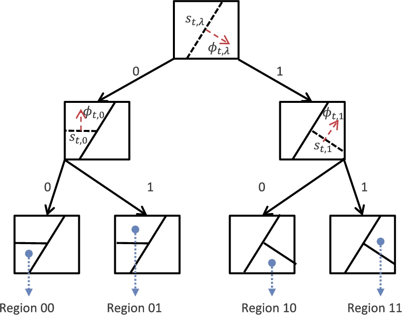
Although nonlinear modeling using trees is a powerful and efficient method, there exist several algorithmic parameters and design choices that affect their performance in many applications [11]. Tuning these parameters is a difficult task for applications involving nonstationary data exhibiting saturation effects, threshold phenomena or chaotic behavior [14]. In particular, the performance of tree-based models heavily depends on a careful partitioning of the feature space. Selection of a good partition is essential to balance the bias and variance of the regressor [12]. As an example, even for a uniform binary tree, while increasing the depth of the tree improves the modeling power, such an increase usually results in overfitting [15]. To address this issue, there exist nonlinear modeling algorithms that avoid such a direct commitment to a particular partition but instead construct a weighted average of all possible partitions (or equivalently, piece-wise models) defined on a tree [6,7,16,17]. Note that a full binary tree of depth d defines a doubly exponential number of different partitions of the feature space [18]; for an example, see Fig. 9.2. Each of these partitions can be represented by a certain collection of the nodes of the tree, where each node represents a particular region of the feature space. Any of these partitions can be used to construct a nonlinear model, e.g., by training a linear model in each region, we can obtain a piece-wise linear model. Instead of selecting one of these partitions and fixing it as the nonlinear model, one can run all partitions in parallel and combine their outputs using a mixture-of-experts approach. Such methods are shown to mitigate the bias–variance tradeoff in a deterministic framework [6,7,16,19]. However, these methods are naturally constrained to work on a fixed partitioning structure, i.e., the partitions are fixed and cannot be adapted to data.

Although there exist numerous methods to partition the feature space, many of these split criteria are typically chosen a priori and fixed such as the dyadic partitioning [20] and a specific loss (e.g., the Gini index [21]) is minimized separately for each node. For instance, multivariate trees are extended to allow the simultaneous use of functional inner and leaf nodes to draw a decision in [13]. Similarly, the node-specific individual decisions are combined in [22] via the context tree weighting method [23] and a piece-wise linear model for sequential classification is obtained. Since the partitions in these methods are fixed and chosen even before the processing starts, the nonlinear modeling capability of such methods is very limited and significantly deteriorates in cases of high dimensionality [24].
To resolve this issue, we introduce self-organizing trees (SOTs) that jointly learn the optimal feature space partitioning to minimize the loss of the algorithm. In particular, we consider a binary tree where a separator (e.g., a hyperplane) is used to bisect the feature space in a nested manner, and an online linear predictor is assigned to each node. The sequential losses of these node predictors are combined (with their corresponding weights that are sequentially learned) into a global loss that is parameterized via the separator functions and the parameters of the node predictors. We minimize this global loss using online gradient descent, i.e., by updating the complete set of SOT parameters, i.e., the separators, the node predictors and the combination weights, at each time instance. The resulting predictor is a highly dynamical SOT structure that jointly (and in an online and adaptive manner) learns the region classifiers and the optimal feature space partitioning and hence provides an efficient nonlinear modeling with multiple learning machines. In this respect, the proposed method is remarkably robust to drifting source statistics, i.e., nonstationarity. Since our approach is essentially based on a finite combination of linear models, it generalizes well and does not overfit or limitedly overfits (as also shown by an extensive set of experiments).
9.2 Self-Organizing Trees for Regression Problems
In this section, we consider the sequential nonlinear regression problem, where we observe a desired signal {dt}t⩾1![]() , dt∈R
, dt∈R![]() , and regression vectors {xt}t⩾1
, and regression vectors {xt}t⩾1![]() , xt∈Rp
, xt∈Rp![]() , such that we sequentially estimate dt
, such that we sequentially estimate dt![]() by
by
ˆdt=ft(xt),
where ft(⋅)![]() is the adaptive nonlinear regression function defined by the SOT. At each time t, the regression error of the algorithm is given by
is the adaptive nonlinear regression function defined by the SOT. At each time t, the regression error of the algorithm is given by
et=dt−ˆdt
and the objective of the algorithm is to minimize the square error loss ∑Tt=1e2t![]() , where T is the number of observed samples.
, where T is the number of observed samples.
9.2.1 Notation
We first introduce a labeling for the tree nodes following [23]. The root node is labeled with an empty binary string λ and assuming that a node has a label n, where n is a binary string, we label its upper and lower children as n1 and n0, respectively. Here we emphasize that a string can only take its letters from the binary alphabet {0,1}![]() , where 0 refers to the lower child and 1 refers to the upper child of a node. We also introduce another concept, i.e., the definition of the prefix of a string. We say that a string n′=q′1…q′l′
, where 0 refers to the lower child and 1 refers to the upper child of a node. We also introduce another concept, i.e., the definition of the prefix of a string. We say that a string n′=q′1…q′l′![]() is a prefix to string n=q1…ql
is a prefix to string n=q1…ql![]() if l′⩽l
if l′⩽l![]() and q′i=qi
and q′i=qi![]() for all i=1,…,l′
for all i=1,…,l′![]() and the empty string λ is a prefix to all strings. Let P(n)
and the empty string λ is a prefix to all strings. Let P(n)![]() represent all prefixes to the string n, i.e., P(n)≜{n0,…,nl}
represent all prefixes to the string n, i.e., P(n)≜{n0,…,nl}![]() , where l≜l(n)
, where l≜l(n)![]() is the length of the string n, ni
is the length of the string n, ni![]() is the string with l(ni)=i
is the string with l(ni)=i![]() and n0=λ
and n0=λ![]() is the empty string, such that the first i letters of the string n form the string ni
is the empty string, such that the first i letters of the string n form the string ni![]() for i=0,…,l
for i=0,…,l![]() .
.
For a given SOT of depth D, we let ND![]() denote all nodes defined on this SOT and LD
denote all nodes defined on this SOT and LD![]() denote all leaf nodes defined on this SOT. We also let βD
denote all leaf nodes defined on this SOT. We also let βD![]() denote the number of partitions defined on this SOT. This yields the recursion βj+1=β2j+1
denote the number of partitions defined on this SOT. This yields the recursion βj+1=β2j+1![]() for all j⩾1
for all j⩾1![]() , with the base case β0=1
, with the base case β0=1![]() . For a given partition k, we let Mk
. For a given partition k, we let Mk![]() denote the set of all nodes in this partition.
denote the set of all nodes in this partition.
For a node n∈ND![]() (defined on the SOT of depth D), we define SD(n)≜{ˊn∈ND|P(ˊn)=n}
(defined on the SOT of depth D), we define SD(n)≜{ˊn∈ND|P(ˊn)=n}![]() as the set of all nodes of the SOT of depth D, whose set of prefixes includes node n.
as the set of all nodes of the SOT of depth D, whose set of prefixes includes node n.
For a node n∈ND![]() (defined on the SOT of depth D) with length l(n)⩾1
(defined on the SOT of depth D) with length l(n)⩾1![]() , the total number of partitions that contain n can be found by the following recursion:
, the total number of partitions that contain n can be found by the following recursion:
γd(l(n))≜l(n)∏j=1βd−j.
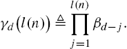
For the case where l(n)=0![]() (i.e., for n=λ
(i.e., for n=λ![]() ), one can clearly observe that there exists only one partition containing λ, therefore γd(0)=1
), one can clearly observe that there exists only one partition containing λ, therefore γd(0)=1![]() .
.
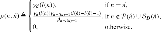
For two nodes n,ˊn∈ND![]() (defined on the SOT of depth D), we let ρ(n,ˊn)
(defined on the SOT of depth D), we let ρ(n,ˊn)![]() denote the number of partitions that contain both n and ˊn
denote the number of partitions that contain both n and ˊn![]() . Trivially, if ˊn=n
. Trivially, if ˊn=n![]() , then ρ(n,ˊn)=γd(l(n))
, then ρ(n,ˊn)=γd(l(n))![]() . If n≠ˊn
. If n≠ˊn![]() , then letting ˉn
, then letting ˉn![]() denote the longest prefix to both n and ˊn
denote the longest prefix to both n and ˊn![]() , i.e., the longest string in P(n)∩P(ˊn)
, i.e., the longest string in P(n)∩P(ˊn)![]() , we obtain
, we obtain
ρ(n,ˊn)≜{γd(l(n)),if n=´n,γd(l(n))γd−l(ˉn)−1(l(ˊn)−l(ˉn)−1)βd−l(ˉn)−1,if n∉P(ˊn)∪SD(ˊn),0,otherwise.
Since l(ˉn)+1⩽l(n)![]() and l(ˉn)+1⩽l(ˊn)
and l(ˉn)+1⩽l(ˊn)![]() from the definition of the SOT, we naturally have ρ(n,ˊn)=ρ(ˊn,n)
from the definition of the SOT, we naturally have ρ(n,ˊn)=ρ(ˊn,n)![]() .
.
9.2.2 Construction of the Algorithm
For each node n on the SOT, we define a node predictor
ˆdt,n=vTt,nxt,
whose parameter vt,n![]() is updated using the online gradient descent algorithm. We also define a separator function for each node p on the SOT except the leaf nodes (note that leaf nodes do not have any children) using the sigmoid function
is updated using the online gradient descent algorithm. We also define a separator function for each node p on the SOT except the leaf nodes (note that leaf nodes do not have any children) using the sigmoid function
st,n=11+exp(ϕTt,nxt),
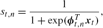
where ϕt,n![]() is the normal to the separation plane. We then define the prediction of any partition according to the hierarchical structure of the SOT as the weighted sum of the prediction of the nodes in that partition, where the weighting is determined by the separator functions of the nodes between the leaf node and the root node. In particular, the prediction of the kth partition at time t is defined as follows:
is the normal to the separation plane. We then define the prediction of any partition according to the hierarchical structure of the SOT as the weighted sum of the prediction of the nodes in that partition, where the weighting is determined by the separator functions of the nodes between the leaf node and the root node. In particular, the prediction of the kth partition at time t is defined as follows:
ˆd(k)t=∑n∈Mk(ˆdt,nl(n)−1∏i=0sqit,ni),
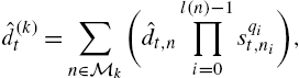
where ni∈P(n)![]() is the prefix to string n with length i−1
is the prefix to string n with length i−1![]() , qi
, qi![]() is the ith letter of the string n, i.e., ni+1=niqi
is the ith letter of the string n, i.e., ni+1=niqi![]() , and finally sqit,ni
, and finally sqit,ni![]() denotes the value of the separator function at node ni
denotes the value of the separator function at node ni![]() such that
such that
sqit,ni≜{st,ni,if qi=0,1−st,ni,otherwise,
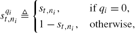
with st,ni![]() defined as in (9.3). We emphasize that we dropped the n dependency of qi
defined as in (9.3). We emphasize that we dropped the n dependency of qi![]() and ni
and ni![]() to simplify notation. Using these definitions, we can construct the final estimate of our algorithm as
to simplify notation. Using these definitions, we can construct the final estimate of our algorithm as
ˆdt=∑k∈βDw(k)tˆd(k)t,
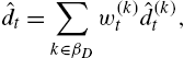
where w(k)t![]() represents the weight of partition k at time t.
represents the weight of partition k at time t.
Having found a method to combine the predictions of all partitions to generate the final prediction of the algorithm, we next aim to obtain a low-complexity representation since there are O(1.52D)![]() different partitions defined on the SOT and (9.6) requires a storage and computational complexity of O(1.52D)
different partitions defined on the SOT and (9.6) requires a storage and computational complexity of O(1.52D)![]() . To this end, we denote the product terms in (9.4) as follows:
. To this end, we denote the product terms in (9.4) as follows:
ˆδt,n≜ˆdt,nl(n)−1∏i=0sqit,ni,
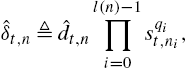
where ˆδt,n![]() can be viewed as the estimate of the node n at time t. Then (9.4) can be rewritten as follows:
can be viewed as the estimate of the node n at time t. Then (9.4) can be rewritten as follows:
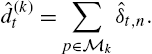
ˆd(k)t=∑p∈Mkˆδt,n.
Since we now have a compact form to represent the tree and the outputs of each partition, we next introduce a method to calculate the combination weights of O(1.52D)![]() partitions in a simplified manner. For this, we assign a particular linear weight to each node. We denote the weight of node n at time t as wt,n
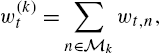
partitions in a simplified manner. For this, we assign a particular linear weight to each node. We denote the weight of node n at time t as wt,n![]() and then define the weight of the kth partition as the sum of the weights of its nodes, i.e.,
and then define the weight of the kth partition as the sum of the weights of its nodes, i.e.,
w(k)t=∑n∈Mkwt,n,
for all k∈{1,…,βD}![]() . Since we use online gradient descent to update the weight of each partition, the weight of partition k is recursively updated as
. Since we use online gradient descent to update the weight of each partition, the weight of partition k is recursively updated as
w(k)t+1=w(k)t+μtetˆd(k)t.
This yields the following recursive update on the node weights:
wt+1,n=wt,n+μtetˆδt,n,
where ˆδt,n![]() is defined as in (9.7). This result implies that instead of managing O(1.52D)
is defined as in (9.7). This result implies that instead of managing O(1.52D)![]() memory locations and making O(1.52D)
memory locations and making O(1.52D)![]() calculations, only keeping track of the weights of every node is sufficient and the number of nodes in a depth-D model is |ND|=2D+1−1
calculations, only keeping track of the weights of every node is sufficient and the number of nodes in a depth-D model is |ND|=2D+1−1![]() . Therefore, we can reduce the storage and computational complexity from O(1.52D)
. Therefore, we can reduce the storage and computational complexity from O(1.52D)![]() to O(2D)
to O(2D)![]() by performing the update in (9.8) for all n∈ND
by performing the update in (9.8) for all n∈ND![]() .
.
Using these node predictors and weights, we construct the final estimate of our algorithm as follows:
ˆdt=βd∑k=1{(∑n∈Mkwt,n)(∑n∈Mkˆδt,n)}.

Here, we observe that for arbitrary two nodes n,ˊn∈Nd![]() , the product wt,nˆδt,ˊn
, the product wt,nˆδt,ˊn![]() appears ρ(n,ˊn)
appears ρ(n,ˊn)![]() times in ˆdt
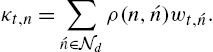
times in ˆdt![]() (cf. (9.1)). Hence, the combination weight of the estimate of the node n at time t can be calculated as follows:
(cf. (9.1)). Hence, the combination weight of the estimate of the node n at time t can be calculated as follows:
κt,n=∑ˊn∈Ndρ(n,ˊn)wt,ˊn.
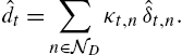
Using the combination weight (9.9), we obtain the final estimate of our algorithm as follows:
ˆdt=∑n∈NDκt,nˆδt,n.
Note that (9.10) is equal to (9.6) with a storage and computational complexity of O(4D)![]() instead of O(1.52D)
instead of O(1.52D)![]() .
.
As we derived all the update rules for the node weights and the parameters of the individual node predictors, what remains is to provide an update scheme for the separator functions. To this end, we use the online gradient descent update
ϕt+1,n=ϕt,n−12ηt∇e2t(ϕt,n),
for all nodes n∈ND∖LD![]() , where ηt
, where ηt![]() is the learning rate of the algorithm and ∇e2t(ϕt,n)
is the learning rate of the algorithm and ∇e2t(ϕt,n)![]() is the derivative of e2t(ϕt,n)
is the derivative of e2t(ϕt,n)![]() with respect to ϕt,n
with respect to ϕt,n![]() . After some algebra, we obtain
. After some algebra, we obtain
ϕt+1,n=ϕt,n+ηtet∂ˆdt∂st,n∂st,n∂ϕt,n=ϕt,n+ηtet{∑ˊn∈NDκt,ˊn∂ˆδt,ˊn∂st,n}∂st,n∂ϕt,n=ϕt,n+ηtet{1∑q=0∑ˊn∈SD(nq)(−1)qκt,ˊnˆδt,ˊnsqt,n}∂st,n∂ϕt,n,

where we use the logistic regression classifier as our separator function, i.e., st,n=(1+exp(xTtϕt,n))−1![]() . Therefore, we have
. Therefore, we have
∂st,n∂ϕt,n=−(1+exp(xTtϕt,n))−2exp(xTtϕt,n)xt=−st,n(1−st,n)xt.
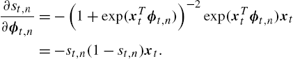
We emphasize that other separator functions can also be used in a similar way by simply calculating the gradient with respect to the extended direction vector and plugging in (9.12) and (9.13). From (9.13), we observe that ∇e2t(ϕt,n)![]() includes the product of st,n
includes the product of st,n![]() and 1−st,n
and 1−st,n![]() terms; hence, in order not to slow down the learning rate of our algorithm, we restrict s+⩽st⩽1−s+
terms; hence, in order not to slow down the learning rate of our algorithm, we restrict s+⩽st⩽1−s+![]() for some 0<s+<0.5
for some 0<s+<0.5![]() . In accordance with this restriction, we define the separator functions as follows:
. In accordance with this restriction, we define the separator functions as follows:
st=s++1−2s+1+exTtϕt.

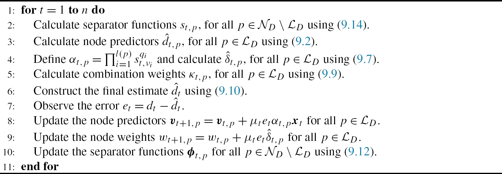
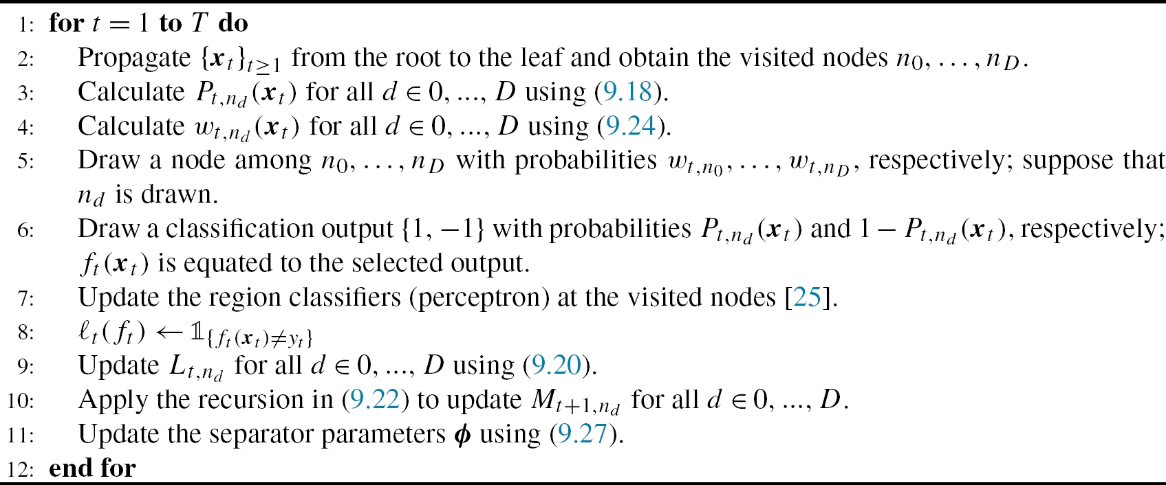
According to the update rule in (9.12), the computational complexity of the introduced algorithm results in O(p4d)![]() . This concludes the construction of the algorithm and a pseudocode is given in Algorithm 1.
. This concludes the construction of the algorithm and a pseudocode is given in Algorithm 1.
9.2.3 Convergence of the Algorithm
For Algorithm 1, we have the following convergence guarantee, which implies that our regressor (given in Algorithm 1) asymptotically achieves the performance of the best linear combination of the O(1.52D)![]() different adaptive models that can be represented using a depth-D tree with a computational complexity O(p4D)
different adaptive models that can be represented using a depth-D tree with a computational complexity O(p4D)![]() . While constructing the algorithm, we refrain from any statistical assumptions on the underlying data, and our algorithm works for any sequence of {dt}t⩾1
. While constructing the algorithm, we refrain from any statistical assumptions on the underlying data, and our algorithm works for any sequence of {dt}t⩾1![]() with an arbitrary length of n. Furthermore, one can use this algorithm to learn the region boundaries and then feed this information to the first algorithm to reduce computational complexity.
with an arbitrary length of n. Furthermore, one can use this algorithm to learn the region boundaries and then feed this information to the first algorithm to reduce computational complexity.
Theorem 1
Let {dt}t⩾1![]() and {xt}t⩾1
and {xt}t⩾1![]() be arbitrary, bounded and real-valued sequences. The predictor ˆdt
be arbitrary, bounded and real-valued sequences. The predictor ˆdt![]() given in Algorithm 1 when applied to these sequences yields
given in Algorithm 1 when applied to these sequences yields
T∑t=1(dt−ˆdt)2−minw∈RβdT∑t=1(dt−wTˆdt)2⩽O(log(T)),
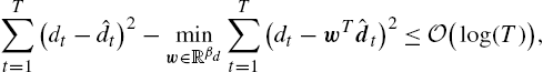
for all T, when e2t(w)![]() is strongly convex ∀t, where ˆdt=[ˆd(1)t,…,ˆd(βd)t]T
is strongly convex ∀t, where ˆdt=[ˆd(1)t,…,ˆd(βd)t]T![]() and ˆd(k)t
and ˆd(k)t![]() represents the estimate of dt
represents the estimate of dt![]() at time t for the adaptive model k=1,…,βd
at time t for the adaptive model k=1,…,βd![]() .
.
Proof of this theorem can be found in Appendix 9.A.1.
9.3 Self-Organizing Trees for Binary Classification Problems
In this section, we study online binary classification, where we observe feature vectors {xt}t⩾1![]() and determine their labels {yt}t⩾1
and determine their labels {yt}t⩾1![]() in an online manner. In particular, the aim is to learn a classification function ft(xt)
in an online manner. In particular, the aim is to learn a classification function ft(xt)![]() with xt∈Rp
with xt∈Rp![]() and yt∈{−1,1}
and yt∈{−1,1}![]() such that, when applied in an online manner to any streaming data, the empirical loss of the classifier ft(⋅)
such that, when applied in an online manner to any streaming data, the empirical loss of the classifier ft(⋅)![]() , i.e.,
, i.e.,
LT(ft)≜T∑t=11{ft(xt)≠dt},

is asymptotically as small (after averaging over T) as the empirical loss of the best partition classifier defined over the SOT of depth D. To be more precise, we measure the relative performance of ft![]() with respect to the performance of a partition classifier f(k)t
with respect to the performance of a partition classifier f(k)t![]() , where k∈{1,…,βD}
, where k∈{1,…,βD}![]() , using the following regret:
, using the following regret:
RT(ft;f(k)t)≜LT(ft)−LT(f(k)t)T,
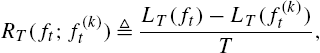
for any arbitrary length T. Our aim is then to construct an online algorithm with guaranteed upper bounds on this regret for any partition classifier defined over the SOT.
9.3.1 Construction of the Algorithm
Using the notations described in Section 9.2.1, the output of a partition classifier k∈{1,…,βD}![]() is constructed as follows. Without loss of generality, suppose that the feature xt
is constructed as follows. Without loss of generality, suppose that the feature xt![]() has fallen into the region represented by the leaf node n∈LD
has fallen into the region represented by the leaf node n∈LD![]() . Then xt
. Then xt![]() is contained in the nodes n0,…,nD
is contained in the nodes n0,…,nD![]() , where nd
, where nd![]() is the i letter prefix of n, i.e., nD=n
is the i letter prefix of n, i.e., nD=n![]() and n0=λ
and n0=λ![]() . For example, if node nd
. For example, if node nd![]() is contained in partition k, then one can simply set f(k)t(xt)=ft,nd(xt)
is contained in partition k, then one can simply set f(k)t(xt)=ft,nd(xt)![]() . Instead of making a hard selection, we allow an error margin for the classification output ft,nd(xt)
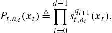
. Instead of making a hard selection, we allow an error margin for the classification output ft,nd(xt)![]() in order to be able to update the region boundaries later in the proof. To achieve this, for each node contained in partition k, we define a parameter called path probability to measure the contribution of each leaf node to the classification task at time t. This parameter is equal to the multiplication of the separator functions of the nodes from the respective node to the root node, which represents the probability that xt
in order to be able to update the region boundaries later in the proof. To achieve this, for each node contained in partition k, we define a parameter called path probability to measure the contribution of each leaf node to the classification task at time t. This parameter is equal to the multiplication of the separator functions of the nodes from the respective node to the root node, which represents the probability that xt![]() should be classified using the region classifier of node nd
should be classified using the region classifier of node nd![]() . This path probability (similar to the node predictor definition in (9.7)) is defined as
. This path probability (similar to the node predictor definition in (9.7)) is defined as
Pt,nd(xt)≜d−1∏i=0sqi+1t,ni(xt),
where pqi+1t,ni(⋅)![]() represents the value of the partitioning function corresponding to node ni
represents the value of the partitioning function corresponding to node ni![]() towards the qi+1
towards the qi+1![]() direction as in (9.5). We consider that the classification output of node nd
direction as in (9.5). We consider that the classification output of node nd![]() can be trusted with a probability of Pt,nd(xt)
can be trusted with a probability of Pt,nd(xt)![]() . This and the other probabilities in our development are independently defined for ease of exposition and gaining intuition, i.e., these probabilities are not related to the unknown data statistics in any way and they definitely cannot be regarded as certain assumptions on the data. Indeed, we do not take any assumptions about the data source.
. This and the other probabilities in our development are independently defined for ease of exposition and gaining intuition, i.e., these probabilities are not related to the unknown data statistics in any way and they definitely cannot be regarded as certain assumptions on the data. Indeed, we do not take any assumptions about the data source.
Intuitively, the path probability is low when the feature vector is close to the region boundaries; hence we may consider to classify that feature vector by another node classifier (e.g., the classifier of the sibling node). Using these path probabilities, we aim to update the region boundaries by learning whether an efficient node classifier is used to classify xt![]() , instead of directly assigning xt
, instead of directly assigning xt![]() to node nd
to node nd![]() and lose a significant degree of freedom. To this end, we define the final output of each node classifier according to a Bernoulli random variable with outcomes {−ft,nd(xt),ft,nd(xt)}
and lose a significant degree of freedom. To this end, we define the final output of each node classifier according to a Bernoulli random variable with outcomes {−ft,nd(xt),ft,nd(xt)}![]() , where the probability of the latter outcome is Pt,nd(xt)
, where the probability of the latter outcome is Pt,nd(xt)![]() . Although the final classification output of node nd
. Although the final classification output of node nd![]() is generated according to this Bernoulli random variable, we continue to call ft,nd(xt)
is generated according to this Bernoulli random variable, we continue to call ft,nd(xt)![]() the final classification output of node nd
the final classification output of node nd![]() , with an abuse of notation. Then the classification output of the partition classifier is set to f(k)t(xt)=ft,nd(xt)
, with an abuse of notation. Then the classification output of the partition classifier is set to f(k)t(xt)=ft,nd(xt)![]() .
.
Before constructing the SOT classifier, we first introduce certain definitions. Let the instantaneous empirical loss of the proposed classifier ft![]() at time t be denoted by ℓt(ft)≜1{ft(xt)≠yt}
at time t be denoted by ℓt(ft)≜1{ft(xt)≠yt}![]() . Then the expected empirical loss of this classifier over a sequence of length T can be found by
. Then the expected empirical loss of this classifier over a sequence of length T can be found by
LT(ft)=E[T∑t=1ℓt(ft)],

with the expectation taken with respect to the randomization parameters of the classifier ft![]() . We also define the effective region of each node nd
. We also define the effective region of each node nd![]() at time t as follows: Rt,nd≜{x:Pt,nd(x)⩾(0.5)d}
at time t as follows: Rt,nd≜{x:Pt,nd(x)⩾(0.5)d}![]() . According to the aforementioned structure of partition classifiers, the node nd
. According to the aforementioned structure of partition classifiers, the node nd![]() classifies an instance xt
classifies an instance xt![]() only if xt∈Rt,nd
only if xt∈Rt,nd![]() . Therefore, the time accumulated empirical loss of any node n during the data stream is given by
. Therefore, the time accumulated empirical loss of any node n during the data stream is given by
LT,n≜∑t⩽T:{xt}t⩾1∈Rt,nℓt(ft,n).

Similarly, the time accumulated empirical loss of a partition classifier k is L(k)T≜∑n∈MkLT,n![]() .
.
We then use a mixture-of-experts approach to achieve the performance of the best partition classifier that minimizes the accumulated classification error. To this end, we set the final classification output of our algorithm as ft(xt)=f(k)t![]() with probability w(k)t
with probability w(k)t![]() , where
, where
w(k)t=1Zt−12−J(k)exp(−bL(k)t−1),
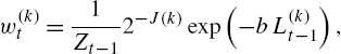
b⩾0![]() is a constant controlling the learning rate of the algorithm, J(k)⩽2|L(k)|−1
is a constant controlling the learning rate of the algorithm, J(k)⩽2|L(k)|−1![]() represents the number of bits required to code the partition k (which satisfies ∑βDk=1J(k)=1
represents the number of bits required to code the partition k (which satisfies ∑βDk=1J(k)=1![]() ) and Zt=∑βDk=12−J(k)exp(−bL(k)t)
) and Zt=∑βDk=12−J(k)exp(−bL(k)t)![]() is the normalization factor.
is the normalization factor.
Although this randomized method can be used as the SOT classifier, in its current form, it requires a computational complexity O(1.52Dp)![]() since the randomization w(k)t
since the randomization w(k)t![]() is performed over the set {1,…,βD}
is performed over the set {1,…,βD}![]() and βD≈1.52D
and βD≈1.52D![]() . However, the set of all possible classification outputs of these partitions has a cardinality as small as D+1
. However, the set of all possible classification outputs of these partitions has a cardinality as small as D+1![]() since xt∈Rt,nD
since xt∈Rt,nD![]() for the corresponding leaf node nD
for the corresponding leaf node nD![]() (in which xt
(in which xt![]() is included) and f(k)t=ft,nd
is included) and f(k)t=ft,nd![]() for some d=0,…,D
for some d=0,…,D![]() , ∀k∈{1,…,βD}
, ∀k∈{1,…,βD}![]() . Hence, evaluating all the partition classifiers in k at the instance xt
. Hence, evaluating all the partition classifiers in k at the instance xt![]() to produce ft(xt)
to produce ft(xt)![]() is unnecessary. In fact, the computational complexity for producing ft(xt)
is unnecessary. In fact, the computational complexity for producing ft(xt)![]() can be reduced from O(1.52Dp)
can be reduced from O(1.52Dp)![]() to O(Dp)
to O(Dp)![]() by performing the exact same randomization over ft,nd
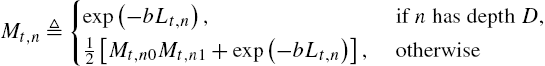
by performing the exact same randomization over ft,nd![]() 's using the new set of weights wt,nd
's using the new set of weights wt,nd![]() , which can be straightforwardly derived as follows:
, which can be straightforwardly derived as follows:
wt,nd=βD∑k=1w(k)t1f(k)t(xt)=ft,nd(xt).
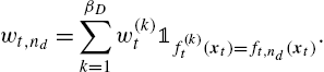
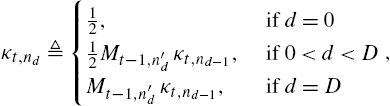
To efficiently calculate (9.21) with complexity O(Dp)![]() , we consider the universal coding scheme and let
, we consider the universal coding scheme and let
Mt,n≜{exp(−bLt,n), ifnhas depthD,12[Mt,n0Mt,n1+exp(−bLt,n)], otherwise
for any node n and observe that we have Mt,λ=Zt![]() [23]. Therefore, we can use the recursion (9.22) to obtain the denominator of the randomization probabilities w(k)t
[23]. Therefore, we can use the recursion (9.22) to obtain the denominator of the randomization probabilities w(k)t![]() . To efficiently calculate the numerator of (9.21), we introduce another intermediate parameter as follows. Letting n′d
. To efficiently calculate the numerator of (9.21), we introduce another intermediate parameter as follows. Letting n′d![]() denote the sibling of node nd
denote the sibling of node nd![]() , we recursively define
, we recursively define
κt,nd≜{12, if d=012Mt−1,n′dκt,nd−1, if 0<d<DMt−1,n′dκt,nd−1, if d=D,
∀d∈{0,…,D}![]() , where xt∈Rt,nD
, where xt∈Rt,nD![]() . Using the intermediate parameters in (9.22) and (9.23), it can be shown that we have
. Using the intermediate parameters in (9.22) and (9.23), it can be shown that we have
wt,nd=κt,ndexp(−bLt,nd)Mt,λ.
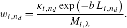
Hence, we obtain the final output of the algorithm as ft(xt)=ft,nd(xt)![]() with probability wt,nd
with probability wt,nd![]() , where d∈{0,…,D}
, where d∈{0,…,D}![]() (i.e., with a computational complexity O(D)
(i.e., with a computational complexity O(D)![]() ).
).
We then use the final output of the introduced algorithm and update the region boundaries of the tree (i.e., organize the tree) to minimize the final classification error. To this end, we minimize the loss E[ℓt(ft)]=E[1{ft(xt)≠yt}]=14E[(yt−ft(xt))2]![]() with respect to the region boundary parameters, i.e., we use the stochastic gradient descent method as follows:
with respect to the region boundary parameters, i.e., we use the stochastic gradient descent method as follows:
ϕt+1,nd=ϕt,nd−η∇E[ℓt(ft)]=ϕt,nd−(−1)qd+1η(yt−ft(xt))sq′d+1t,nd(xt)[D∑i=d+1ft,ni(xt)]xt,
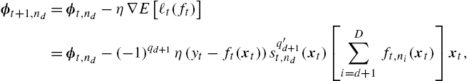
∀d∈{0,…,D−1}![]() , where η denotes the learning rate of the algorithm and q′d+1
, where η denotes the learning rate of the algorithm and q′d+1![]() represents the complementary letter to qd+1
represents the complementary letter to qd+1![]() from the binary alphabet {0,1}
from the binary alphabet {0,1}![]() . Defining a new intermediate variable
. Defining a new intermediate variable
πt,nd≜{ft,nd(xt), if d=D−1,πt,nd+1+ft,nd(xt), if d<D−1,
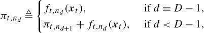
one can perform the update in (9.25) with a computational complexity O(p)![]() for each node nd
for each node nd![]() , where d∈{0,…,D−1}
, where d∈{0,…,D−1}![]() , resulting in an overall computational complexity of O(Dp)
, resulting in an overall computational complexity of O(Dp)![]() as follows:
as follows:
ϕt+1,nd=ϕt,nd−(−1)md+1η(yt−ft(xt))πt,ndsq′d+1t,nd(xt)xt.
This concludes the construction of the algorithm and the pseudocode of the SOT classifier can be found in Algorithm 2.
9.3.2 Convergence of the Algorithm
In this section, we illustrate that the performance of Algorithm 2 is asymptotically as good as the best partition classifier such that, as T→∞![]() , we have RT(ft;f(k)t)→0
, we have RT(ft;f(k)t)→0![]() . Hence, Algorithm 2 asymptotically achieves the performance of the best partition classifier among O(1.52D)
. Hence, Algorithm 2 asymptotically achieves the performance of the best partition classifier among O(1.52D)![]() different classifiers that can be represented using the SOT of depth D with a significantly reduced computational complexity of O(Dp)
different classifiers that can be represented using the SOT of depth D with a significantly reduced computational complexity of O(Dp)![]() without any statistical assumptions on data.
without any statistical assumptions on data.
Theorem 2
Let {xt}t⩾1![]() and {yt}t⩾1
and {yt}t⩾1![]() be arbitrary and real-valued sequences of feature vectors and their labels, respectively. Then Algorithm 2, when applied to these data sequences, sequentially yields
be arbitrary and real-valued sequences of feature vectors and their labels, respectively. Then Algorithm 2, when applied to these data sequences, sequentially yields
maxk∈{1,…,βD}E[RT(ft;f(k)t)]⩽O(√2DT),
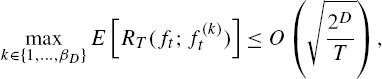
for all T with a computational complexity O(Dp)![]() , where p represents the dimensionality of the feature vectors and the expectation is with respect to the randomization parameters.
, where p represents the dimensionality of the feature vectors and the expectation is with respect to the randomization parameters.
Proof of this theorem can be found in Appendix 9.A.2.
9.4 Numerical Results
In this section, we illustrate the performance of SOTs under different scenarios with respect to state-of-the-art methods. The proposed method has a wide variety of application areas, such as channel equalization [26], underwater communications [27], nonlinear modeling in big data [28], speech and texture analysis [29, Chapter 7] and health monitoring [30]. Yet, in this section, we consider nonlinear modeling for fundamental regression and classification problems.
9.4.1 Numerical Results for Regression Problems
Throughout this section, “SOTR” represents the self-organizing tree regressor defined in Algorithm 1, “CTW” represents the context tree weighting algorithm of [16], “OBR” represents the optimal batch regressor, “VF” represents the truncated Volterra filter [1], “LF” represents the simple linear filter, “B-SAF” and “CR-SAF” represent the Beizer and the Catmull–Rom spline adaptive filter of [2], respectively, and “FNF” and “EMFNF” represent the Fourier and even mirror Fourier nonlinear filter of [3], respectively. Finally, “GKR” represents the Gaussian-kernel regressor and it is constructed using n node regressors, say ˆdt,1,…,ˆdt,n![]() , and a fixed Gaussian mixture weighting (that is selected according to the underlying sequence in hindsight), giving
, and a fixed Gaussian mixture weighting (that is selected according to the underlying sequence in hindsight), giving
ˆdt=n∑i=1f(xt;μi,Σi)ˆdt,i,
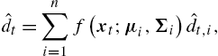
where ˆdt,i=vTt,ixt![]() and
and
f(xt;μi,Σi)≜12π√|Σi|e−12(xt−μi)TΣ−1i(xt−μi),
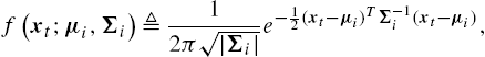
for all i=1,…,n![]() .
.
For a fair performance comparison, in the corresponding experiments in Subsection 9.4.1.2, the desired data and the regressor vectors are normalized between [−1,1]![]() since the satisfactory performance of several algorithms requires the knowledge on the upper bounds (such as the B-SAF and the CR-SAF) and some require these upper bounds to be between [−1,1]
since the satisfactory performance of several algorithms requires the knowledge on the upper bounds (such as the B-SAF and the CR-SAF) and some require these upper bounds to be between [−1,1]![]() (such as the FNF and the EMFNF). Moreover, in the corresponding experiments in Subsection 9.4.1.1, the desired data and the regressor vectors are normalized between [−1,1]
(such as the FNF and the EMFNF). Moreover, in the corresponding experiments in Subsection 9.4.1.1, the desired data and the regressor vectors are normalized between [−1,1]![]() for the VF, the FNF and the EMFNF algorithms due to the aforementioned reason. The regression errors of these algorithms are then scaled back to their original values for a fair comparison.
for the VF, the FNF and the EMFNF algorithms due to the aforementioned reason. The regression errors of these algorithms are then scaled back to their original values for a fair comparison.
Considering the illustrated examples in the respective papers [2,3,16], the orders of the FNF and the EMFNF are set to 3 for the experiments in Subsection 9.4.1.1 and 2 for the experiments in Subsection 9.4.1.2. The order of the VF is set to 2 for all experiments. Similarly, the depth of the trees for the SOTR and CTW algorithms is set to 2 for all experiments. For these tree-based algorithms, the feature space is initially partitioned by the direction vectors ϕt,n=[ϕ(1)t,n,…,ϕ(p)t,n]T![]() for all nodes n∈ND∖LD
for all nodes n∈ND∖LD![]() , where ϕ(i)t,n=−1
, where ϕ(i)t,n=−1![]() if i≡l(n)(modD)
if i≡l(n)(modD)![]() , e.g., when D=p=2
, e.g., when D=p=2![]() , we have the four quadrants as the four leaf nodes of the tree. Finally, we use cubic B-SAF and CR-SAF algorithms, whose number of knots are set to 21 for all experiments. We emphasize that both these parameters and the learning rates of these algorithms are selected to give equal rates of performance and convergence.
, we have the four quadrants as the four leaf nodes of the tree. Finally, we use cubic B-SAF and CR-SAF algorithms, whose number of knots are set to 21 for all experiments. We emphasize that both these parameters and the learning rates of these algorithms are selected to give equal rates of performance and convergence.
9.4.1.1 Mismatched Partitions
In this subsection, we consider the case where the desired data is generated by a piece-wise linear model that mismatches with the initial partitioning of the tree-based algorithms. Specifically, the desired signal is generated by the following piece-wise linear model:
dt={wTxt+πt,if ϕT0xt⩾0.5 and ϕT1xt⩾1,−wTxt+πt,if ϕT0xt⩾0.5 and ϕT1xt<1,−wTxt+πt,if ϕT0xt<0.5 and ϕT2xt⩾−1,wTxt+πt,if ϕT0xt<0.5 and ϕT2xt<−1,

where w=[1,1]T![]() , ϕ0=[4,−1]T
, ϕ0=[4,−1]T![]() , ϕ1=[1,1]T
, ϕ1=[1,1]T![]() , ϕ2=[1,2]T
, ϕ2=[1,2]T![]() , xt=[x1,t,x2,t]T
, xt=[x1,t,x2,t]T![]() , πt
, πt![]() is a sample function from a zero mean white Gaussian process with variance 0.1 and x1,t
is a sample function from a zero mean white Gaussian process with variance 0.1 and x1,t![]() and x2,t
and x2,t![]() are sample functions of a jointly Gaussian process of mean [0,0]T
are sample functions of a jointly Gaussian process of mean [0,0]T![]() and variance I2
and variance I2![]() . The learning rates are set to 0.005 for SOTR and CTW, 0.1 for FNF, 0.025 for B-SAF and CR-SAF, 0.05 for EMFNF and VF. Moreover, in order to match the underlying partition, the mass points of GKR are set to μ1=[1.4565,1.0203]T
. The learning rates are set to 0.005 for SOTR and CTW, 0.1 for FNF, 0.025 for B-SAF and CR-SAF, 0.05 for EMFNF and VF. Moreover, in order to match the underlying partition, the mass points of GKR are set to μ1=[1.4565,1.0203]T![]() , μ2=[0.6203,−0.4565]T
, μ2=[0.6203,−0.4565]T![]() , μ3=[−0.5013,0.5903]T
, μ3=[−0.5013,0.5903]T![]() and μ4=[−1.0903,−1.0013]T
and μ4=[−1.0903,−1.0013]T![]() with the same covariance matrix as in the previous example.
with the same covariance matrix as in the previous example.
Fig. 9.3 shows the normalized time accumulated regression error of the proposed algorithms. We emphasize that the SOTR algorithm achieves a better error performance compared to its competitors. Comparing the performances of the SOTR and CTW algorithms, we observe that the CTW algorithm fails to accurately predict the desired data, whereas the SOTR algorithm learns the underlying partitioning of the data, which significantly improves the performance of the SOTR. This illustrates the importance of the initial partitioning of the regressor space for tree-based algorithms to yield a satisfactory performance.
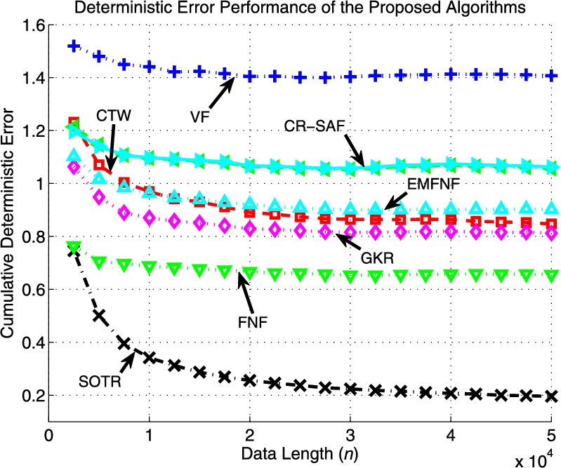
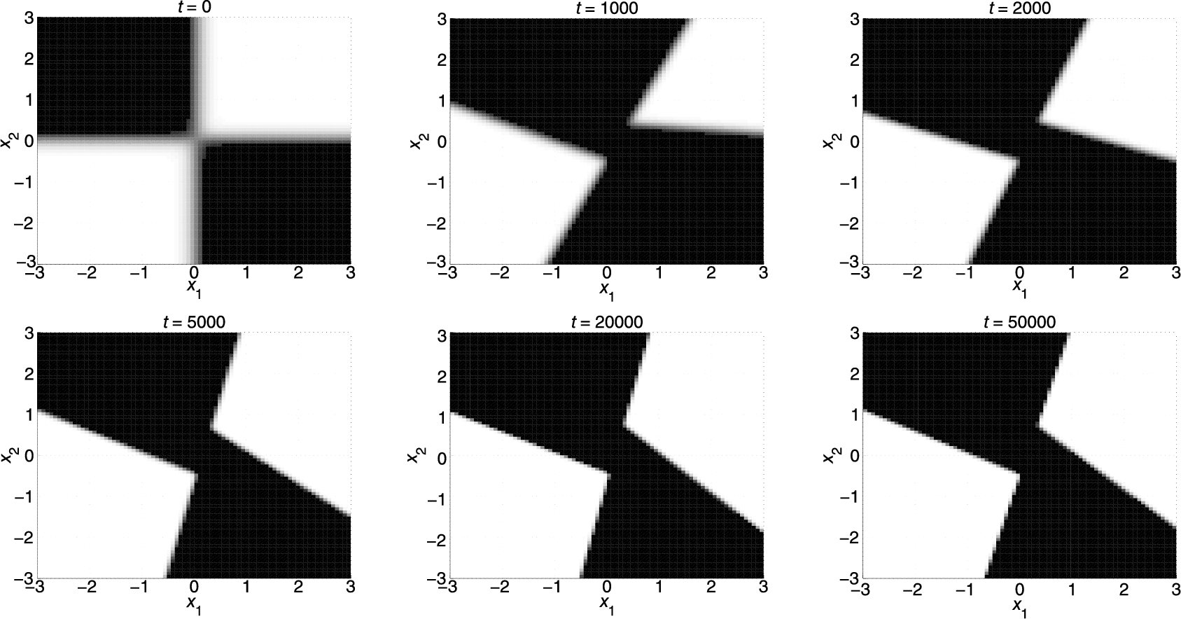
In particular, the CTW algorithm converges to the best batch regressor having the predetermined leaf nodes (i.e., the best regressor having the four quadrants of two-dimensional space as its leaf nodes). However that regressor is suboptimal since the underlying data is generated using another constellation; hence its time accumulated regression error is always lower bounded by O(1)![]() compared to the global optimal regressor. The SOTR algorithm, on the other hand, adapts its region boundaries and captures the underlying unevenly rotated and shifted regressor space partitioning perfectly. Fig. 9.4 shows how our algorithm updates its separator functions and illustrates the nonlinear modeling power of SOTs.
compared to the global optimal regressor. The SOTR algorithm, on the other hand, adapts its region boundaries and captures the underlying unevenly rotated and shifted regressor space partitioning perfectly. Fig. 9.4 shows how our algorithm updates its separator functions and illustrates the nonlinear modeling power of SOTs.
9.4.1.2 Chaotic Signals
In this subsection, we illustrate the performance of the SOTR algorithm when estimating chaotic data generated by the Henon map and the Lorenz attractor [31].
First, we consider a zero mean sequence generated by the Henon map, a chaotic process given by
dt=1−ζd2t−1+ηdt−2,
known to exhibit chaotic behavior for the values of ζ=1.4![]() and η=0.3
and η=0.3![]() . The desired data at time t is denoted as dt
. The desired data at time t is denoted as dt![]() whereas the extended regressor vector is xt=[dt−1,dt−2,1]T
whereas the extended regressor vector is xt=[dt−1,dt−2,1]T![]() , i.e., we consider a prediction framework. The learning rate is set to 0.025 for B-SAF and CR-SAF, whereas it is set to 0.05 for the rest.
, i.e., we consider a prediction framework. The learning rate is set to 0.025 for B-SAF and CR-SAF, whereas it is set to 0.05 for the rest.
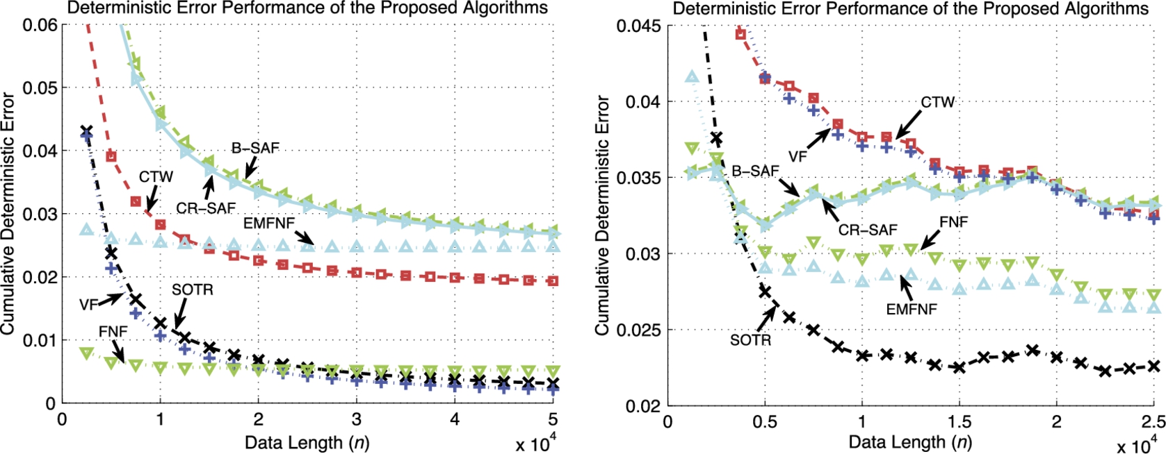
Fig. 9.5 (left plot) shows the normalized regression error performance of the proposed algorithms. One can observe that the algorithms whose basis functions do not include the necessary quadratic terms and the algorithms that rely on a fixed regressor space partitioning yield unsatisfactory performance. On the other hand, VF can capture the salient characteristics of this chaotic process since its order is set to 2. Similarly, FNF can also learn the desired data since its basis functions can well approximate the chaotic process. The SOTR algorithm, however, uses a piece-wise linear modeling and still achieves asymptotically the same performance as the VF algorithm, while outperforming the FNF algorithm.
Second, we consider the chaotic signal set generated using the Lorenz attractor [31] that is defined by the following three discrete-time equations:
xt=xt−1+(σ(y−x))dt,yt=yt−1+(xt−1(ρ−zt−1)−yt−1)dt,zt=zt−1+(xt−1yt−1−βzt−1)dt,
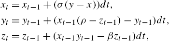
where we set dt=0.01![]() , ρ=28
, ρ=28![]() , σ=10
, σ=10![]() and β=8/3
and β=8/3![]() to generate the well-known chaotic solution of the Lorenz attractor. In the experiment, xt
to generate the well-known chaotic solution of the Lorenz attractor. In the experiment, xt![]() is selected as the desired data and the two-dimensional region represented by yt,zt
is selected as the desired data and the two-dimensional region represented by yt,zt![]() is set as the regressor space, that is, we try to estimate xt
is set as the regressor space, that is, we try to estimate xt![]() with respect to yt
with respect to yt![]() and zt
and zt![]() . The learning rates are set to 0.01 for all algorithms.
. The learning rates are set to 0.01 for all algorithms.
Fig. 9.5 (right plot) illustrates the nonlinear modeling power of the SOTR algorithm even when estimating a highly nonlinear chaotic signal set. As can be observed from Fig. 9.5, the SOTR algorithm significantly outperforms its competitors and achieves a superior error performance since it tunes its region boundaries to the optimal partitioning of the regressor space, whereas the performances of the other algorithms directly rely on the initial selection of the basis functions and/or tree structures and partitioning.
9.4.2 Numerical Results for Classification Problems
9.4.2.1 Stationary Data
In this section, we consider stationary classification problems and compare the SOTC algorithm with the following methods: Perceptron, “PER” [25]; Online AdaBoost, “OZAB” [32]; Online GradientBoost, “OGB” [33]; Online SmoothBoost, “OSB” [34]; and Online Tree–Based Nonadaptive Competitive Classification, “TNC” [22]. The parameters for all of these compared methods are set as in their original proposals. For “OGB” [33], which uses K weak learners per M selectors, essentially resulting in MK weak learners in total, we use K=1![]() , as in [34], for a fair comparison along with the logit loss that has been shown to consistently outperform other choices in [33]. The TNC algorithm is nonadaptive, i.e., not self-organizing, in terms of the space partitioning, which we use in our comparisons to illustrate the gain due to the proposed self-organizing structure. We use the Perceptron algorithm as the weak learners and node classifiers in all algorithms. We set the learning rate of the SOTC algorithm to η=0.05
, as in [34], for a fair comparison along with the logit loss that has been shown to consistently outperform other choices in [33]. The TNC algorithm is nonadaptive, i.e., not self-organizing, in terms of the space partitioning, which we use in our comparisons to illustrate the gain due to the proposed self-organizing structure. We use the Perceptron algorithm as the weak learners and node classifiers in all algorithms. We set the learning rate of the SOTC algorithm to η=0.05![]() in all of our stationary as well as nonstationary data experiments. We use N=100
in all of our stationary as well as nonstationary data experiments. We use N=100![]() weak learners for the boosting methods, whereas we use a depth-4 tree in SOTC and TNC algorithms, which corresponds to 31=25−1
weak learners for the boosting methods, whereas we use a depth-4 tree in SOTC and TNC algorithms, which corresponds to 31=25−1![]() local node classifiers. The SOTC algorithm has linear complexity in the depth of the tree, whereas the compared methods have linear complexity in the number of weak learners.
local node classifiers. The SOTC algorithm has linear complexity in the depth of the tree, whereas the compared methods have linear complexity in the number of weak learners.
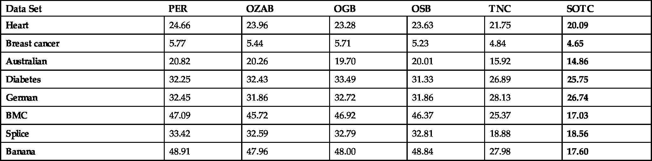
As can be observed in Table 9.1, the SOTC algorithm consistently outperforms the compared methods. In particular, the compared methods essentially fail to classify Banana and BMC datasets, which indicates that these methods are not able to extend to complex nonlinear classification problems. On the contrary, the SOTC algorithm successfully models these complex nonlinear relations with piece-wise linear curves and provides a superior performance. In general, the SOTC algorithm has significantly better transient characteristics and the TNC algorithm occasionally performs poorly (such as on BMC and Banana data sets) depending on the mismatch between the initial partitions defined on the tree and the underlying optimal separation of the data. This illustrates the importance of learning the region boundaries in piece-wise linear models.
Table 9.1
Average classification errors (in percentage) of algorithms on benchmark datasets
| Data Set | PER | OZAB | OGB | OSB | TNC | SOTC |
|---|---|---|---|---|---|---|
| Heart | 24.66 | 23.96 | 23.28 | 23.63 | 21.75 | 20.09 |
| Breast cancer | 5.77 | 5.44 | 5.71 | 5.23 | 4.84 | 4.65 |
| Australian | 20.82 | 20.26 | 19.70 | 20.01 | 15.92 | 14.86 |
| Diabetes | 32.25 | 32.43 | 33.49 | 31.33 | 26.89 | 25.75 |
| German | 32.45 | 31.86 | 32.72 | 31.86 | 28.13 | 26.74 |
| BMC | 47.09 | 45.72 | 46.92 | 46.37 | 25.37 | 17.03 |
| Splice | 33.42 | 32.59 | 32.79 | 32.81 | 18.88 | 18.56 |
| Banana | 48.91 | 47.96 | 48.00 | 48.84 | 27.98 | 17.60 |
9.4.2.2 Nonstationary Data: Concept Change/Drift
In this section, we apply the SOTC algorithm to nonstationary data, where there might be continuous or sudden/abrupt changes in the source statistics, i.e., concept change. Since the SOTC algorithm processes data in a sequential manner, we choose the Dynamically Weighted Majority (DWM) algorithm (DWM) [35] with Perceptron (DWM-P) or naive Bayes (DWM-N) experts for the comparison, since the DWM algorithm is also an online algorithm. Although the batch algorithms do not truly fit into our framework, we still devise an online version of the tree-based local space partitioning algorithm [24] (which also learns the space partitioning and the classifier using the coordinate ascent approach) using a sliding-window approach and abbreviate it as the WLSP algorithm. For the DWM method, which allows the addition and removal of experts during the stream, we set the initial number of experts to 1, where the maximum number of experts is bounded by 100. For the WLSP method, we use a window size of 100. The parameters for these compared methods are set as in their original proposals.
We run these methods on the BMC dataset (1200 instances, Fig. 9.6), where a sudden/abrupt concept change is obtained by rotating the feature vectors (clock-wise around the origin) 180∘![]() after the 600th instance. This is effectively equivalent to flipping the label of the feature vectors; hence the resulting dataset is denoted as BMC-F. For a continuous concept drift, we rotate each feature vector 180∘/1200=0.15∘
after the 600th instance. This is effectively equivalent to flipping the label of the feature vectors; hence the resulting dataset is denoted as BMC-F. For a continuous concept drift, we rotate each feature vector 180∘/1200=0.15∘![]() starting from the beginning; the resulting dataset is denoted as BMC-C. In Fig. 9.6, we present the classification errors for the compared methods averaged over 1000 trials. At each 10th instance, we test the algorithms with 1200 instances drawn from the active set of statistics (active concept).
starting from the beginning; the resulting dataset is denoted as BMC-C. In Fig. 9.6, we present the classification errors for the compared methods averaged over 1000 trials. At each 10th instance, we test the algorithms with 1200 instances drawn from the active set of statistics (active concept).

Since the BMC dataset is non-Gaussian with strongly nonlinear class separations, the DWM method does not perform well on the BMC-F data. For instance, DWM-P operates with an error rate fluctuating around 0.48–0.49 (random guess). This results since the performance of the DWM method is directly dependent on the expert success and we observe that both base learners (Perceptron or the naive Bayes) fail due to the high separation complexity in the BMC-F data. On the other hand, the WLSP method quickly converges to steady state, however it is also asymptotically outperformed by the SOTC algorithm in both experiments. Increasing the window size is clearly expected to boost the performance of WLSP, however at the expense of an increased computational complexity. It is already significantly slower than the SOTC method even when the window size is 100 (for a more detailed comparison, see Table 9.2). The performance of the WLSP method is significantly worse on the BMC-C data set compared to the BMC-F data set, since in the former scenario, WLSP is trained with batch data of a continuous mixture of concepts in the sliding windows. Under this continuous concept drift, the SOTC method always (not only asymptotically as in the case of the BMC-F data set) performs better than the WLSP method. Hence, the sliding-window approach is sensitive to the continuous drift. Our discussion about the DWM method on the concept change data (BMC-F) remains valid in the case of the concept drift (BMC-C) as well. In these experiments, the power of self-organizing trees is obvious as the SOTC algorithm almost always outperforms the TNC algorithm. We also observe from Table 9.2 that the SOTC algorithm is computationally very efficient and the cost of region updates (compared to the TNC algorithm) does not increase the computational complexity of the algorithm significantly.
Table 9.2
Running times (in seconds) of the compared methods when processing the BMC data set on a daily-use machine (Intel(R) Core(TM) i5-3317U CPU @ 1.70 GHz with 4 GB memory)
| PER | OZAB | OGB | OSB | TNC | DWM-P | DWM-N | WLSP | SOTC |
|---|---|---|---|---|---|---|---|---|
| 0.06 | 12.90 | 3.57 | 3.91 | 0.43 | 2.06 | 6.91 | 68.40 | 0.62 |

Appendix 9.A
9.A.1 Proof of Theorem 1
For the SOT of depth D, suppose ˆd(k)t![]() , k=1,…,βd
, k=1,…,βd![]() , are obtained as described in Section 9.2.2. To achieve the upper bound in (9.15), we use the online gradient descent method and update the combination weights as
, are obtained as described in Section 9.2.2. To achieve the upper bound in (9.15), we use the online gradient descent method and update the combination weights as
wt+1=wt−12ηt∇e2t(wt)=wt+ηtetˆdt,
where ηt![]() is the learning rate of the online gradient descent algorithm. We derive an upper bound on the sequential learning regret Rn
is the learning rate of the online gradient descent algorithm. We derive an upper bound on the sequential learning regret Rn![]() , which is defined as
, which is defined as
RT≜T∑t=1e2t(wt)−T∑t=1e2t(w⁎n),
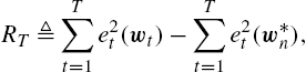
where w⁎T![]() is the optimal weight vector over T, i.e.,
is the optimal weight vector over T, i.e.,
w⁎T≜argminw∈RβdT∑t=1e2t(w).

Following [36], using Taylor series approximation, for some point zt![]() on the line segment connecting wt
on the line segment connecting wt![]() to w⁎T
to w⁎T![]() , we have
, we have
e2t(w⁎T)=e2t(wt)+(∇e2t(wt))T(w⁎T−wt)+12(w⁎T−wt)T∇2e2t(zt)(w⁎T−wt).
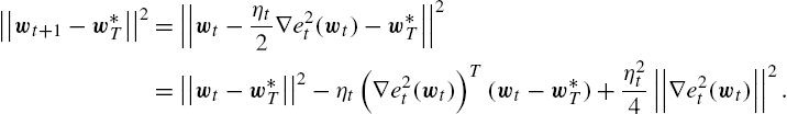
According to the update rule in (9.32), at each iteration the update on weights are performed as wt+1=wt−ηt2∇e2t(wt)![]() . Hence, we have
. Hence, we have
||wt+1−w⁎T||2=||wt−ηt2∇e2t(wt)−w⁎T||2=||wt−w⁎T||2−ηt(∇e2t(wt))T(wt−w⁎T)+η2t4||∇e2t(wt)||2.
This yields
(∇e2t(wt))T(wt−w⁎T)=||wt−w⁎T||2−||wt+1−w⁎T||2ηt+ηt||∇e2t(wt)||24.

Under the mild assumptions that ||∇e2t(wt)||2⩽A2![]() for some A>0
for some A>0![]() and e2t(w⁎T)
and e2t(w⁎T)![]() is λ-strong convex for some λ>0
is λ-strong convex for some λ>0![]() [36], we achieve the following upper bound:
[36], we achieve the following upper bound:
e2t(wt)−e2t(w⁎T)⩽||wt−w⁎T||2−||wt+1−w⁎T||2ηt−λ2||wt−w⁎T||2+ηtA24.

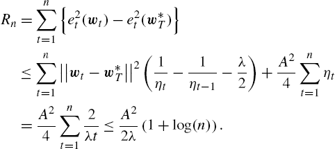
By selecting ηt=2λt![]() and summing up the regret terms in (9.34), we get
and summing up the regret terms in (9.34), we get
Rn=n∑t=1{e2t(wt)−e2t(w⁎T)}⩽n∑t=1||wt−w⁎T||2(1ηt−1ηt−1−λ2)+A24n∑t=1ηt=A24n∑t=12λt⩽A22λ(1+log(n)).
9.A.2 Proof of Theorem 2
Since Zt![]() is a summation of terms that are all positive, we have Zt⩾2−J(k)exp(−bL(k)t)
is a summation of terms that are all positive, we have Zt⩾2−J(k)exp(−bL(k)t)![]() and after taking the logarithm of both sides and rearranging the terms, we get
and after taking the logarithm of both sides and rearranging the terms, we get
−1blogZT⩽L(k)T+J(k)log2b
for all k∈{1,…,βD}![]() at the (last) iteration at time T. We then make the following observation:
at the (last) iteration at time T. We then make the following observation:
ZT=T∏t=1ZtZt−1=T∏t=1βD∑k=12−J(k)exp(−bL(k)t−1)Zt−1exp(−bℓt(f(k)t))⩽exp(−bLT(ft)+Tb28),
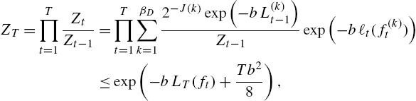
where the second line follows from the definition of Zt![]() and the last line follows from the Hoeffding inequality by treating the w(k)t=2−J(k)exp(−bL(k)t−1)/Zt−1
and the last line follows from the Hoeffding inequality by treating the w(k)t=2−J(k)exp(−bL(k)t−1)/Zt−1![]() terms as the randomization probabilities. Note that LT(ft)
terms as the randomization probabilities. Note that LT(ft)![]() represents the expected loss of the final algorithm; cf. (9.19). Combining (9.35) and (9.36), we obtain
represents the expected loss of the final algorithm; cf. (9.19). Combining (9.35) and (9.36), we obtain
LT(ft)T⩽L(k)TT+J(k)log2Tb+b8
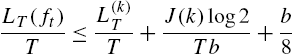
and choosing b=√2D/T![]() , we find the desired upper bound in (9.28) since J(k)⩽2D+1−1
, we find the desired upper bound in (9.28) since J(k)⩽2D+1−1![]() , for all k∈{1,…,βD}
, for all k∈{1,…,βD}![]() .
.