
2.1 Introduction
In this chapter, I present algorithms for the adaptive solutions of matrix algebra problems from a sequence of matrices. The streams or sequences can be random matrices {Ak} or {Bk}, or the correlation matrices of random vector sequences {xk} or {yk}. Examples of matrix algebra are matrix inversion, square root, inverse square root, eigenvectors, generalized eigenvectors, singular vectors, and generalized singular vectors.
This chapter additionally covers the basic terminologies and methods used throughout the remaining chapters. I also present well-known adaptive algorithms to compute the mean, median, covariance, inverse covariance, and correlation matrices from random matrix or vector sequences. Furthermore, I present a new algorithm to compute the normalized mean of a random vector sequence.
For the sake of simplicity, let’s assume that the multidimensional data {xk∈ℜn} arrives as a sequence. From this data sequence, we can derive a matrix sequence { }. We define the data correlation matrix A as follows:
![$$ A=underset{k o infty }{lim }Eleft[{mathbf{x}}_k{mathbf{x}}_k^T
ight] $$](https://imgdetail.ebookreading.net/2023/10/9781484280171/9781484280171__9781484280171__files__images__522202_1_En_2_Chapter__522202_1_En_2_Chapter_TeX_IEq2.png) . (2.1)
. (2.1)
2.2 Stationary and Non-Stationary Sequences
![$$ {lim}_{k o infty }Eleft[{mathbf{x}}_k{mathbf{x}}_k^T
ight] $$](https://imgdetail.ebookreading.net/2023/10/9781484280171/9781484280171__9781484280171__files__images__522202_1_En_2_Chapter__522202_1_En_2_Chapter_TeX_IEq3.png) is a constant. For a non-stationary sequence {xk},
is a constant. For a non-stationary sequence {xk}, ![$$ Eleft[{mathbf{x}}_k{mathbf{x}}_{k+m}^T
ight] $$](https://imgdetail.ebookreading.net/2023/10/9781484280171/9781484280171__9781484280171__files__images__522202_1_En_2_Chapter__522202_1_En_2_Chapter_TeX_IEq4.png) remains a function of both k and m, and
remains a function of both k and m, and ![$$ Eleft[{mathbf{x}}_k{mathbf{x}}_k^T
ight] $$](https://imgdetail.ebookreading.net/2023/10/9781484280171/9781484280171__9781484280171__files__images__522202_1_En_2_Chapter__522202_1_En_2_Chapter_TeX_IEq5.png) is a function of k. Examples of non-stationary data are given in Publicly Real-World Datasets to Evaluate Stream Learning Algorithms [Vinicius Souza et al. 20]. Figure 2-1 shows examples of stationary and non-stationary data.
is a function of k. Examples of non-stationary data are given in Publicly Real-World Datasets to Evaluate Stream Learning Algorithms [Vinicius Souza et al. 20]. Figure 2-1 shows examples of stationary and non-stationary data.

Examples of stationary and non-stationary data
Non-stationarity in data can be detected by well-known techniques described in this reference [Shay Palachy 19].
2.3 Use Cases for Adaptive Mean, Median, and Covariances
Adaptive mean computation is important in real-world applications even though it is one of the simplest algorithms.
Handwritten Character Recognition
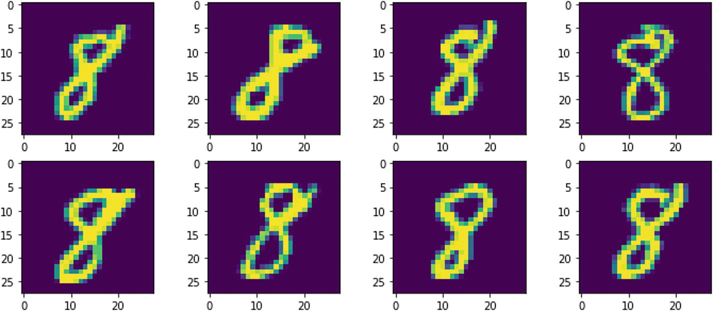
Examples of variations in handwritten number 8
One algorithm to recognize the number 8 with all its variations is to find the mean set of pixels that represent it. Due to random variations in handwriting, it is difficult to compile all variations of each character ahead of time. It is important to design an adaptive learning scheme whereby instantaneous variations in these characters are immediately represented in the machine learning algorithm.


Anomaly Detection of Streaming Data

Anomalies detected with an adaptive median algorithm on time series data
More on this topic is discussed in Chapter 8.
2.4 Adaptive Mean and Covariance of Nonstationary Sequences
In the stationary case, given a sequence {xk∈ℜn}, we can compute the adaptive mean mk as follows:
 . (2.2)
Similarly, the adaptive correlation Ak is
 . (2.3)
Here we use all samples up to time instant k.
If, however, the data is non-stationary, we use a forgetting factor 0<β≤1 to implement an effective window of size 1/(1–β) as
 (2.4)
(2.4)
and
 . (2.5)
This effective window ensures that the past data samples are downweighted with an exponentially fading window compared to the recent ones in order to afford the tracking capability of the adaptive algorithm. The exact value of β depends on the specific application. Generally speaking, for slow time-varying {xk}, β is chosen close to 1 to implement a large effective window, whereas for fast time-varying {xk}, β is chosen near zero for a small effective window [Benveniste et al. 90].
2.5 Adaptive Covariance and Inverses
Given the mean and correlations discussed before, the adaptive covariance matrix Bk can also be computed as follows:
 (2.6)
(2.6)
From the adaptive correlation matrix Ak in (2.5), the inverse correlation matrix  can be obtained adaptively by the Sherman-Morrison formula [Sherman–Morrison, Wikipedia] as
 . (2.7)
Similarly, the inverse covariance matrix  can be obtained adaptively as
 . (2.8)
2.6 Adaptive Normalized Mean Algorithm
The most obvious choice for an adaptive normalized mean algorithm is to use (2.2) and normalize each mk. However, a more efficient algorithm can be obtained from the following cost function whose minimizer w* is the asymptotic normalized mean m/‖m‖, where m = limk → ∞E[xk]:
 , (2.9)
where α is a Lagrange multiplier that enforces the constraint that the mean is normalized. The gradient of J(wk;xk) with respect to wk is
 . (2.10)
Multiplying (2.10) by  and applying the constraint
  , we obtain
 . (2.11)
Using this α in (2.11), we obtain the adaptive gradient descent algorithm for normalized mean:
 , (2.12)
where ηk is a small decreasing constant, which follows assumption A1.2 in the Proofs of Convergence in GitHub [Chatterjee GitHub].
Variations of the Adaptive Normalized Mean Algorithm
There are several variations of the objective function (2.9) that lead to many other adaptive algorithms for normalized mean computation. One variation of (2.9) is to place the value of α in (2.11) in the objective function (2.9) to obtain the following objective function:
 . (2.13)
Unlike (2.9), this objective function is unconstrained and has the constraint  built into it. It leads to the following adaptive algorithm:
 . (2.14)
Another variation is the use of a penalty function method of nonlinear optimization that enforces the constraint  . This objective function is
 , (2.15)
where μ is a positive penalty constant. This objective function is also unconstrained and leads to the following adaptive algorithm:
 . (2.16)
2.7 Adaptive Median Algorithm
Given a sequence {xk}, its asymptotic median μ satisfies the following:
 (2.17)
where P(E) is the probability measure of event E and 0 ≤ P(E) ≤ 1. The objective function J(wk;xk) whose minimizer w* is the asymptotic median μ is
J(wk; xk) = ‖xk − wk‖. (2.18)
The gradient of J(wk;xk) with respect to wk is
 , (2.19)
where sgn(.) is the sign operator (sgn(x)=1 if x≥0 and –1 if x<0). From the gradient in (2.19), we obtain the adaptive gradient descent algorithm:
wk + 1 = wk + ηk sgn (xk − wk). (2.20)
2.8 Experimental Results
The purpose of these experiments is to demonstrate the performance and accuracies of the adaptive algorithms for mean, correlation, inverse correlation, inverse covariance, normalized mean, and median.
I generated 1,000 sample vectors {xk} of five-dimensional Gaussian data (i.e., n=5) with the following mean and covariance:
Mean = [10 7 6 5 1],
Covariance =  .
.

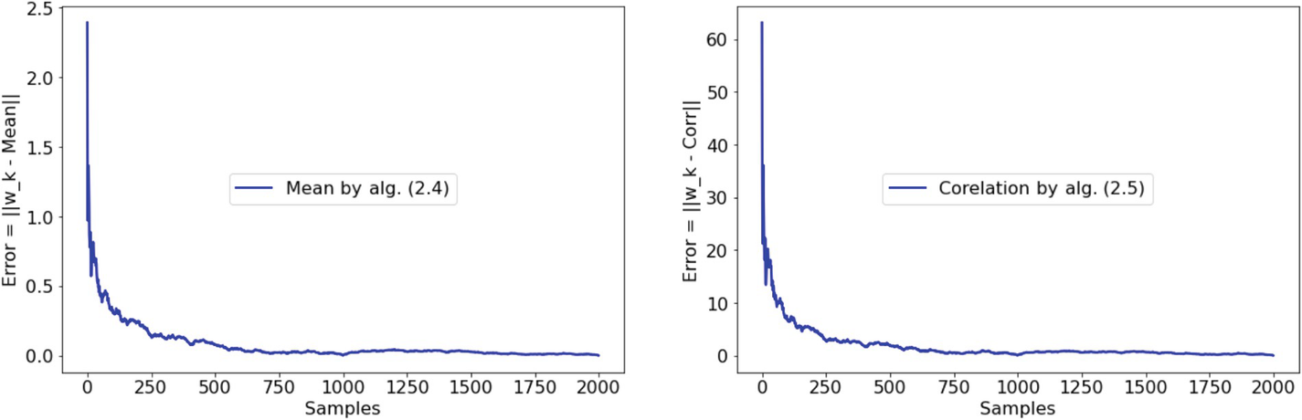


All adaptive algorithms converged rapidly. After the 1,000 samples were processed, the errors were 0.0043 for algorithms (2.14) and (2.16), and 0.0408 for algorithm (2.20). See the code in the GitHub repository [Chatterjee GitHub].