
3.1 Introduction and Use Cases
Adaptive computation of the square root and inverse square root of the real-time correlation matrix of a streaming sequence {xk∈ℜn} has numerous applications in machine learning, data analysis, and image/signal processing. They include data whitening, classifier design, and data normalization [Foley and Sammon 75; Fukunaga 90].
To transform correlated noise in a signal to independent and identically distributed (iid) noise, which is easier to classify
Generalized eigenvector computation [Chatterjee et al. Mar 97] (see Chapter 7)
Linear discriminant analysis computation [linear discriminant analysis, Wikipedia]
Gaussian classifier design and computation of distance measures [Chatterjee et al. May 97]

Original correlated data on the left and the uncorrelated “whitened” data on the right


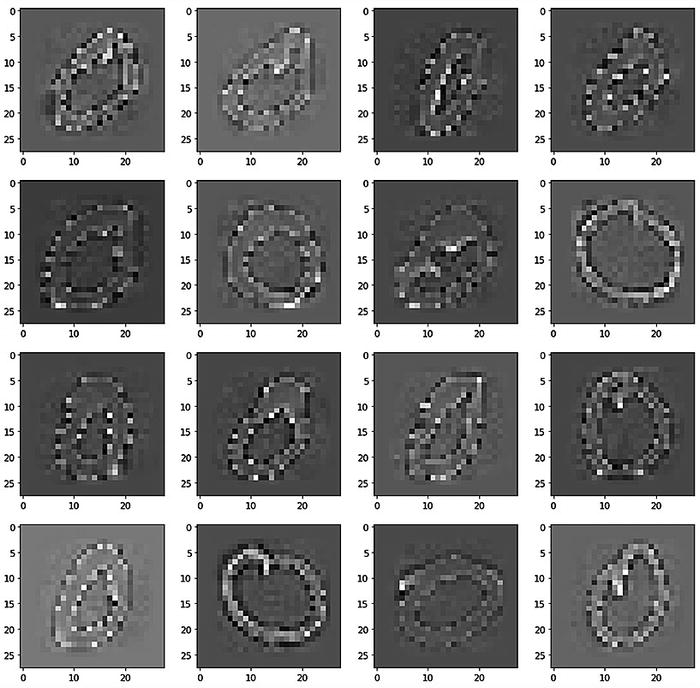
Handwritten MNIST number 0 and the correlation matrix of all characters

Handwritten MNIST number 0 after whitening. The correlation matrix of all characters is diagonal

The square root of A, also called the Cholesky decomposition [Cholesky decomposition, Wikipedia], is denoted by A½. Similarly, A–½ denotes the inverse square root of A. However, as explained below, there is no unique solution for both of these matrix functions, and various adaptive algorithms can be obtained where each algorithm leads to a different solution. Even though there are numerous solutions for these matrix functions, there are unique solutions under some restrictions, such as a unique symmetric positive definite solution.
In this chapter, I present three adaptive algorithms for each matrix function A½ and A–½. Out of the three, one adaptive algorithm leads to the symmetric positive definite solution and two lead to more general solutions.
Various Solutions for A½ and A–½
Let
A=ΦΛΦT be the eigen-decomposition of the real, symmetric, positive definite nXn matrix A, where Φ and Λ are respectively the eigenvector and eigenvalue matrices of A. Here Λ=diag(λ1,…,λn) is the diagonal eigenvalue matrix with λ1≥…≥λn>0, and Φ∈ℜnXn is orthonormal. A solution for A½ is L=ΦD, where D= . However, in general this is not a symmetric solution, and for any orthonormal1 matrix U, ΦDU is also a solution. We can show that A½ is symmetric if, and only if, it is of the form ΦDΦT, and there are 2n symmetric solutions for A½. When D is positive definite, we obtain the unique symmetric positive definite solution for A½ as ΦΛ½ΦT, where Λ½ =
  . Similarly, a general solution for the inverse square root A–½ of A is ΦD–1U, where D is defined before and U is any orthonormal matrix. The unique symmetric positive definite solution for A–½ is ΦΛ–½ΦT, where Λ–½ =
 .
.
Outline of This Chapter
In sections 3.2, 3.3, and 3.4, I discuss three algorithms for the adaptive computation of A½. Section 3.4 discusses the unique symmetric positive definite solution for A½. In Sections 3.5, 3.6, and 3.7, I discuss three algorithms for the adaptive computation of A–½. Section 3.7 describes the unique symmetric positive definite solution for A–½. Section 3.8 presents experimental results for the six algorithms with 10-dimensional Gaussian data. Section 3.9 concludes the chapter.
3.2 Adaptive Square Root Algorithm: Method 1
Let {xk∈ℜn} be a sequence of data vectors whose online data correlation matrix Ak∈ℜnXn is given by
 . (3.1)
Here xk is an observation vector at time k and 0<β≤1 is a forgetting factor used for non-stationary sequences. If the data is stationary, the asymptotic correlation matrix A is
![$$ A=underset{k o infty }{lim }Eleft[{A}_k
ight] $$](https://imgdetail.ebookreading.net/2023/10/9781484280171/9781484280171__9781484280171__files__images__522202_1_En_3_Chapter__522202_1_En_3_Chapter_TeX_IEq5.png) . (3.2)
. (3.2)
Objective Function
Following the methodology described in Section 1.4, I present the algorithm by first showing an objective function J, whose minimum with respect to matrix W gives us the square root of the asymptotic data correlation matrix A. The objective function is
 . (3.3)
The gradient of J(W) with respect to W is
∇WJ(W) = − 4W(A − WTW). (3.4)
Adaptive Algorithm
From the gradient in (3.4), we obtain the following adaptive gradient descent algorithm:
 , (3.5)
where ηk is a small decreasing constant and follows assumption A1.2 in the Proofs of Convergence in the GitHub [Chatterjee GitHub].
3.3 Adaptive Square Root Algorithm: Method 2
Objective Function
The objective function J(W), whose minimum with respect to W gives us the square root of A, is
 . (3.6)
The gradient of J(W) with respect to W is
∇WJ(W) = − 4(A − WWT )W. (3.7)
Adaptive Algorithm
We obtain the following adaptive gradient descent algorithm for square root of A:
 , (3.8)
where ηk is a small decreasing constant.
3.4 Adaptive Square Root Algorithm: Method 3
Adaptive Algorithm
Following the adaptive algorithms (3.5) and (3.8), I now present an algorithm for the computation of a symmetric positive definite square root of A:
 , (3.9)
where ηk is a small decreasing constant and Wk is symmetric.
3.5 Adaptive Inverse Square Root Algorithm: Method 1
Objective Function
The objective function J(W), whose minimizer W* gives us the inverse square root of A, is
 . (3.10)
The gradient of J(W) with respect to W is
∇WJ(W) = − 4AW(I − WTAW). (3.11)
Adaptive Algorithm
From the gradient in (3.11), we obtain the following adaptive gradient descent algorithm:
 (3.12)
3.6 Adaptive Inverse Square Root Algorithm: Method 2
Objective Function
The objective function J(W), whose minimum with respect to W gives us the inverse square root of A, is
 . (3.13)
The gradient of J(W) with respect to W is
∇WJ(W) = − 4(I − WAWT)WA. (3.14)
Adaptive Algorithm
We obtain the following adaptive algorithm for the inverse square root of A:
 , (3.15)
where ηk is a small decreasing constant.
3.7 Adaptive Inverse Square Root Algorithm: Method 3
Adaptive Algorithm
By extending the adaptive algorithms (3.12) and (3.15), I now present an adaptive algorithm for the computation of a symmetric positive definite inverse square root of A:
Wk + 1 = Wk + ηk(I − WkAkWk), (3.16)
where ηk is a small decreasing constant and Wk is symmetric.
3.8 Experimental Results
I generated 500 samples {xk} of 10-dimensional (i.e., n=10) Gaussian data with mean zero and covariance, given below. The covariance matrix is obtained from the first covariance matrix in [Okada and Tomita 85] multiplied by 3. The covariance matrix is

The eigenvalues of the covariance matrix are
[17.699, 8.347, 5.126, 3.088, 1.181, 0.882, 0.261, 0.213, 0.182, 0.151].
Experiments for Adaptive Square Root Algorithms

I started the algorithms with W0=I (10X10 identity matrix). At kth update of each algorithm, I computed the Frobenius norm [Frobenius norm, Wikipedia] of the error between the actual correlation matrix A and the square of Wk that is appropriate for each method. I denote this error by ek as follows:
 , (3.17)
 , (3.18)
 , (3.19)
 . (3.20)

It is clear from Figure 3-4 that the errors are all close to zero. The small differences compared to the actual values are due to random fluctuations in the elements of Wk caused by the varying input data.
Experiments for Adaptive Inverse Square Root Algorithms
I used adaptive algorithms (3.12), (3.15), and (3.16) for Methods 1, 2, and 3, respectively, to compute the inverse square root A. I started the algorithms with W0=I (10X10 identity matrix). At kth update of each algorithm, I computed the Frobenius norm of the error between the actual correlation matrix A and the inverse square of Wk that is appropriate for each method. I denoted this error by ek as shown:
 , (3.21)
 , (3.22)
 , (3.23)
 , (3.24)

It is clear from Figure 3-5 that the errors are all close to zero. As before, experiments with higher epochs show an improvement in the estimation accuracy.
3.9 Concluding Remarks
I presented six adaptive algorithms for the computation of the square root and inverse square root of the correlation matrix of a random vector sequence. In four cases, I presented an objective function and, in all cases, I discussed the convergence properties of the algorithms. Note that although I applied the gradient descent technique on these objective functions, I could have applied any other technique of nonlinear optimization such as steepest descent, conjugate direction, Newton-Raphson, or recursive least squares. The availability of the objective functions allows us to derive new algorithms by using new optimization techniques on them, and also to perform convergence analyses of the adaptive algorithms.