- Solving the problem of indexing data according to multiple criteria
- Understanding the treap data structure
- Keeping a binary search tree balanced
- Using treaps to implement balanced binary search trees (BST)
- Working with Randomized Treaps (RT)
- Comparing plain BSTs and RTs
In chapter 2 we saw how it is possible to store elements and retrieve them based on their priorities by using heaps, and how we can improve over binary heaps by using a larger branching factor.
Priority queues are especially useful when we need to consume elements in a certain order from a dynamically changing list (such as the list of tasks to run on a CPU), so that at any time we can get the next element (according to a certain criterion), remove it from the list, and (usually) stop worrying about fixing anything for the other elements. The difference with a sorted list is that we only go through elements in a priority queue once, and the elements already removed from the list won’t matter for the ordering anymore.
Instead, if we need to keep track of the ordering of elements and to possibly go through them more than once (such as a list of objects to render on a web page), priority queues might not be the best choice. Moreover, there are other kinds of operations that we might need to perform; for example, efficiently retrieving the minimum or maximum element of our collection, accessing the i-th element (without removing all elements before it), or finding the predecessor or successor of an element in our ordering.
In appendix C we discuss how trees are the best compromise when we care about all these operations, in addition to insertion and removal. If a tree is balanced, we can perform any of these actions in logarithmic time.
The issue is that trees in general and binary trees in particular are not guaranteed to be balanced. Figure 3.1 shows how, depending on the order of insertion, we might have very balanced or very skewed trees.

Figure 3.1 All possible layouts for BSTs of size 3. The layout depends on the order in which elements are inserted. Notice how two of the sequences produce identical layouts: for [2, 1, 3] and [2, 3, 1] we get the same final result.
In this chapter, we are going to explore a way to use heaps’ properties to be (reasonably) sure we have balanced binary trees.
To explain how this works we will introduce treaps, a hybrid between trees and heaps; however, we are going to take a different approach to treaps that is somewhat unusual in the literature on this data structure.
But first, as always, let’s start by introducing a problem that we would like to solve.
3.1 Problem: Multi-indexing
Your family runs a small grocery shop, and you’d like to help your parents keep up with the inventory. To impress your family and show everyone those computer science classes are worth the effort, you embark on the task of designing a digital inventory management tool, an archive for stock keeping, with two requirements:
-
Be able to (efficiently) search products by name so you can update the stock.
-
Get, at any time, the product with the lowest items in stock, so that you are able to plan your next order.
Of course, you could just buy an off-the-shelf spreadsheet, but where would the fun be in that? Moreover, would anybody be really impressed with that? So, here we go, designing an in-memory data structure that can be queried according to two different criteria.
Clearly, real-world scenarios are more complex than this.You can imagine that each product requires a different time to be shipped to you, that some products are ordered from the same vendors (and therefore you might want to group them in the same order to save on shipment costs), that a product’s price may and will vary with time (so you can choose the cheapest brand for, say, brakes or suspensions), and even that some products might be unavailable sometimes.
All this complexity, however, can be captured in a heuristic function, a score that is computed keeping in mind all the nuances of your business. Conceptually, you can handle that score in the same exact way as the simple inventory count, so you can keep things simple in our example and just use that.
One way to handle these requirements could be by using two different data structures: one for efficient search by name, for instance a hash table, and a priority queue to get the item which most urgently needs to be resupplied.
We will see in chapter 7 that sometimes combining two data structures for a goal is the best choice. This is not the time yet; for now you need to keep in mind the issues in coordinating two such containers, and also that you will likely need more than twice the memory.
Both considerations are kind of worrying; wouldn’t it be nice if there was a single data structure that could handle both aspects natively and efficiently?
3.1.1 The gist of the solution
Let’s be clear about what we are seeking here: it’s not just a matter of optimizing all the operations on a container, like we discuss in appendix C. Here each bit of data, each entry in the container, is made of two separate parts, and both can be “measured” in some way. There are the names of each product, which can be sorted alphabetically, and the number of items we have in stock, that’s also associated with each product: quantities that can be compared to each other to determine which products are scarcer and most urgent to resupply.
Now, if we sort the list of entries according to one criterion—for example, the name—we need to scan the whole list to find a given value for the other criterion, in this case the quantity in stock.
And if we use a min-heap with the scarcer products at its top, then (as we learned in chapter 2) we will also need linear time to scan the whole heap looking for a product to update.
Long story short, none of the basic data structures we describe in appendix C, nor a priority queue, can single-handedly solve our problem.
3.2 Solution: Description and API
Now that we have an idea of what our ideal container should do (but we still don’t know how it should do it), we can define an abstract data structure (ADT ) with the appropriate API. As long as our implementations will abide by this API, we can use any of them seamlessly in an application, or as part of a more complex algorithm, without having to worry about breaking anything (see table 3.1).
Table 3.1 API and contract for SortedPriorityQueue
To that end, we can imagine an extension of priority queues that also keeps its elements sorted. In the rest of the chapter, we will use the term key to refer to elements, and associate a priority to each element.
With respect to the PriorityQueue ADT that we introduced in chapter 2, this SortedPriorityQueue class has a few new methods: a search method to find a given key in the container and two methods returning the minimum and maximum key stored.
If you look at appendix C, you can see that these three operations are usually implemented by many basic data structures, such as linked lists, arrays, or trees (some of them in linear time and others with better performance, offering logarithmic methods).
Thus, we can think about our SortedPriorityQueue as a melting pot between two different containers, integrating both data structures’ characteristics and providing methods from both of them. For instance, it could be thought of as a fusion between heaps and linked lists, or . . .
3.3 Treap
. . . between a tree and a heap!
Treap1 is just the portmanteau2 of tree and heap. Binary search trees, in fact, offer the best average performance across all standard operations: insert, remove, and search (and also min and max).
Heaps, on the other hand, allow us to efficiently keep track of priorities using a tree-like structure. Since binary heaps are also binary trees, the two structures seem compatible; we only need to find a way to make them co-exist in the same structure, and we could get the best of both.
It’s easier said than done, however! If we have a set of unidimensional data, we can’t enforce BST’s and heap’s invariants at the same time:
-
Either we add a “horizontal” constraint (given a node
N, with two childrenL, its left child, andR, its right child, then all keys in the left subtree—rooted atL—must be smaller thanN’s key, and all keys in the right subtree—rooted atR—must be larger thanN’s key). -
Or we add a “vertical” constraint: the key in the root of any subtree must be the smallest of the subtree.
Anyway, we are in luck, because each of our entries has two values: its name and the stock inventory. The idea, therefore, is to enforce BST’s constraints on the names, and heap’s constraint on the quantities, obtaining something like figure 3.2.
In this example, product names are treated as the keys of a binary search tree, so they define a total ordering (from left to right in the figure).
The inventory quantities, instead, are treated as priorities of a heap, so they define a partial ordering from top to bottom. For priorities, like all heaps, we have a partial ordering, meaning that only nodes on the same path from root to leaves are ordered with respect to their priority. In figure 3.2 you can see that children nodes always have a higher stock count than their parents, but there is no ordering between siblings.

Figure 3.2 An example of a treap, with strings as BST keys and integers as heap priorities. Note that the heap, in this case, is a min-heap, so smaller numbers go on top. For a few links close to the root, we also show the range of keys that can be hosted in the tree’s branch rooted at the node they point to.
This kind of tree offers an easy way to query entries by key (by the product names, in the example). While we can’t easily run a query on priorities, we can efficiently locate the element with the highest priority.3 It will always be at the root of the tree!
Extracting the top element however . . . it’s going to be more complicated than with heaps! We can’t just replace it with a heap’s leaf and push it down, because we need to take into account the BST’s constraints as well.
Likewise, when we insert (or delete) a node, we can’t just use the simple BST algorithm. If we just search for the position that the new key would hold in the tree and add it as a leaf, as shown in figure 3.3, the BST constraint will still be abided by, but the new node’s priority might violate the heap’s invariants.

Figure 3.3 An example of the insertion of a node in a treap, based on the keys ordering only. The priority of the new node, however, violates the heap constraints.
Listing 3.1 introduces a possible implementation for the treap’s main structure. We will use an auxiliary class to model the tree’s nodes, and this will be instrumental in our implementation. You might have noticed we are using explicit links to the node’s children, differently from what we did with heaps in chapter 2. We’ll go back to discussing this choice in more detail in section 3.3.2.
class Node
  key
  #type double
  priority

  #type Node
  left
  #type Node
  right
  #type Node
  parent

  function Node(key, priority)                    ❶
    (this.key, this.priority) ← (key, priority)
    this.left ← null
    this.right ← null
    this.parent ← null

  function setLeft(node)                          ❷
    this.left ← node
    if node != null then
      node.parent ← this

class Treap
  #type Node
  root

  function Treap()
    root ← null
❶ The constructor for the class Node sets the key and priority to the arguments and null for all links.
❷ Updates the left child of a Node. This also takes care of updating the parent reference for the children. Method setRight, not shown for the sake of space, works symmetrically.
In this implementation, the Treap class is mostly a wrapper for the root of the actual tree; each node of the tree holds two attributes for a key (that can be of any type, as long as there is a total ordering defined on the possible values) and a priority, that we’ll assume to be a double precision number in this case. (An integer or any type with a total ordering could work too, but we’ll see in the next section that a double works better.)
Moreover, nodes will hold pointers (or references) to two children, left and right, and their parent.
The constructor for a node will just set the key and priority attributes from its arguments, and initialize left and right pointers to null, effectively creating a leaf. The two branches can then be set after construction, or, alternatively, an overloaded version of the constructor also taking the two children can be provided.
3.3.1 Rotations
How do we get out of the impasse? There is one operation on binary search trees that can help us: rotations. Figure 3.4 illustrates how rotations can heal (or break!) the constraints on a treap. Rotations are common operations on many versions of BSTs, such as red-black trees or 2-3 trees.4

Figure 3.4 Left and right rotations illustrated on an example. The treap on the left violates heap’s invariants, and a right rotation on the node marked as X can fix it. Conversely, if we apply a left rotation to the node marked with Y in the heap on the right, the result will break heap’s constraints. Notice how right rotation is always applied to left children, and left rotation to right children.
A rotation, in a binary search tree, is a transformation whose goal is inverting the parent-child relation between two nodes of the tree, Y and X in figure 3.4. We want the child node to become the parent node and vice versa, but we can’t just swap those two nodes: otherwise, in the general case where the keys of the two nodes are different, we would end up violating the ordering of keys.
Instead, what we need to do is remove the whole subtree rooted at the parent, replace it with the (smaller) subtree rooted at the child, and then find a way to plug back in the removed nodes in this new subtree.
How are we going to do that? As you can see in figure 3.4, first we need to distinguish two cases, depending on whether the child node is a left or a right child. The two cases are symmetrical, so we’ll mainly focus on the former.
Listings 3.2 and 3.3 show the pseudocode for right and left rotations, explicating the details of the operations we described a few lines prior. Figure 3.5 illustrates the steps needed for right rotations, where the child node X, the pivot of the rotation, is the left child of its parent Y.
We need to remove Y from the tree, update Y’s parent P (lines #4–11), replacing Y with node X as its child (either left or right, see lines #8-#11); at this point, Y is disconnected from the tree, and with Y its whole right subtree.
function rightRotate(treap, x)          ❶
  if x == null or isRoot(x) then        ❷
    throw
  y ← x.parent                          ❸
  throw-if y.left != x                  ❹
  p  ← y.parent                         ❺
  if p != null then                     ❻
    if p.left == y then                 ❼
      p.setLeft(x)                      ❽
    else
      p.setRight(x)
  else                                  ❾
    treap.root ← x
  y.setLeft(x.right)                    ❿
  x.setRight(y)                         ⓫
❶ Method rightRotate takes a Treap node x and performs a right rotation. It returns nothing, but it has side effects on the treap.
❷ Checks if x is null or the root of the tree. If it is, there is an error. Arguably, we can just return instead of throwing, but swallowing exceptions is usually not a good idea. Method isRoot is left to the reader to implement. (It’s easy, since the root is the only node in a tree without a parent.)
❸ Uses a convenience variable for x’s parent. Since x is not the root of the tree, y won’t be null (so, no need for an extra check).
❹ We can only perform a right rotation on a left child; so if x is y’s right child, there is an error.
❺ Uses a convenience variable for y’s parent
❻ This time we don’t know if p is null or not, so we need to check.
❼ Once we know p is not null, we still don’t know if y is its left or right child.
❽ If there is a parent for y, we need to update it, replacing y with x. Methods setLeft and setRight take care of updating all the links, as shown in listing 3.1.
❾ If, instead, p is null, it means that y was the treap’s root, so we need to update the tree, making x its new root.
❿ Now that a reference to x is stored (either as p’s child or as the new root), we can update y’s left subtree, that will now point to x’s former right subtree.
⓫ Finally, we reconnect y to the tree by setting it as x’s new right child.
Y’s left subtree, instead, is empty because we disconnected X and moved it. We can then move X’s right subtree and assign it to Y’s left child (line #14), as shown in the lower-left section of figure 3.5. This certainly doesn’t violate the key ordering, because (assuming there was no violation before the rotation) key[Y]>=key[Y.left] and key[Y]>=key[Y.left.right]. In other words, since X was the left child of node Y, then the right subtree of node X is still in Y’s left subtree, and all keys in a node’s left subtree are smaller, or at most equal, to the node’s own key. You can also use figure 3.2 as a reference.

Figure 3.5 The algorithm for performing a right rotation on a BST illustrated
All that’s left to do now is reconnect Y to the main tree: we can assign it to X’s right child (line #15), and we won’t have any violation. In fact, we already know that Y (and its right sub-tree) have larger keys than X’s, and for what concerns Y’s left subtree, it was constructed using the former right subtree of X, and by definition all those keys too are larger than X’s.
We saw how to perform a rotation. It’s nothing fancy; it’s just about updating a few links in the tree. The only mystery at this point might be, why is it called a rotation?
Figure 3.6 tries to answer this question, interpreting the steps we saw in listing 3.2 and figure 3.5 from a different point of view. Let me remark that this is just an informal way to illustrate how a rotation works. When you are going to implement this method, you’d better refer to listing 3.2 and figure 3.5.
function lefttRotate(treap, x)      ❶
  if x == null or isRoot(x) then    ❷
    throw
  y ← x.parent                      ❸
  throw-if y.right != x             ❹
  p ← y.parent                      ❺
  if p != null then                 ❻
    if p.left == y then             ❼
      p.setLeft(x)                  ❽
    else
      p.setRight(x)
  else                              ❾
    treap.root ← x
  y.setRight(x.left)                ❿
  x.setLeft(y)                      ⓫
❶ Method leftRotate takes a Treap node x and performs a left rotation. It returns nothing but it has side effects on the treap.
❷ Checks if x is null or the root of the tree. If so, there is an error.
❸ Uses a convenience variable for x’s parent. Since x is not the root of the tree, y won’t be null.
❹ We can only perform a left rotation on a right child. If x is y’s left child, there is an error.
❺ Uses a convenience variable for y’s parent
❻ We don’t know if p is null or not, so we need to check.
❼ Once we know p is not null, we still don’t know if y is its left or right child.
❽ If there is a parent for y, we need to update it, replacing y with x. Methods setLeft and setRight take care of updating all the links, as shown in listing 3.1.
❾ If, instead, p is null, it means that y was the treap’s root, so we need to update the tree making x its new root.
❿ Now that a reference to x is stored (either as p’s child or as the new root), we can update y’s right subtree to point to x’s former left subtree.
⓫ Finally, we reconnect y to the tree by setting it as x’s new left child.
First, let’s assume we call rotate on node X, and node Y is X’s parent. Once again, we analyze right rotation, so X is a left child of Y.
If we consider the subtree rooted at Y, we can visually “rotate” it clockwise (hence “right rotation”), pivoting on node X, until X looks like the root of this tree; hence, all other nodes appear to be below X, as shown in figure 3.6.
The result should look something like the top-right quadrant of figure 3.6. Of course, in order for this to be a valid BST rooted at node X, we need to make a few changes. For instance, there seems to be an edge from a child to its parent, from Y to X: but that’s not allowed in trees, so we need to revert the direction of the edge. If we just did that, though, X would end up with three children, and that’s also not allowed in a binary tree; to fix it, we can transfer the link between X and its right child to Y. Both changes are shown in the bottom-left portion of figure 3.6.

Figure 3.6 A more intuitive interpretation of the rightRotate operation that helps explain its name and also helps with memorizing its steps
At this point, the subtree is structurally fixed, and as a last step we can just enhance its visual representation to make it also look a little better.
You can imagine the tree structure like some kind of bolt and strings dangling structure, and then the whole operation can be described as grabbing the tree by node X and letting all the other nodes dangle from it, with the caveat that we need to also move X’s right child to node Y.
Before closing the discussion on rotations, it’s important to note that rotations always preserve BST constraints, but they do not preserve heap’s invariants. Rotations, in fact, can be used to fix broken treaps, but if applied to a valid tree, they will break the priority constraints on the node to which they are applied.
3.3.2 A few design questions
Treaps are heaps, which in turn are special trees with a dual array representation. As we saw in chapter 2, we can implement a heap using an array, a more space-efficient representation that also exploits locality of reference.
Can we also implement a treap using an array? I encourage you to take a minute and think about this question, before moving on and reading the answer. What would be the pros and cons of using an array versus a tree, and what could be the pain points of using a tree?
The issue with the array representation is that it’s not particularly flexible. It works well if we only swap random elements and remove/add only from the array’s tail; if, instead, we need to move elements around, it’s a disaster! For instance, even inserting a new element in the middle of the array causes all the elements after it to be moved, for an average O(n) swaps (see figure 3.7).

Figure 3.7 When a new element is inserted in an ordered array, all the elements larger than the new one must be shifted one position toward the tail of the array (provided there is still room). This means that if the array has n elements and the new value will be stored at index k (that is, it will be the (k+1)-th element in the array), then n-k assignments will be needed to complete the insertion.
The key point with heaps is that they are complete, balanced, and left-aligned trees, which is possible because heaps don’t keep a total ordering on keys, so we can add and remove elements from the tail of the array, and then bubble up/push down a single element of the heap to reinstate the heap’s properties (see chapter 2).
Treaps, on the other hand, are also binary search trees, which do keep a total ordering on keys. That’s why we need rotations when we insert or delete new elements from a treap. As we described in section 3.2.1, a rotation implies moving a whole subtree from the right subtree of a node X to the left subtree of its parent Y (or vice versa). As you can imagine, this is the kind of operation that is easily performed in constant time when using pointers on a tree’s nodes, but it can become excruciatingly painful on arrays (like, linear-time painful).
And that’s why the array representation is not used for treaps (or for BSTs).
Another design question you might ask (and also should ask) before getting on with the implementation concerns the branching factor for the heap. We saw in chapter 2 that heaps can have branching factors other than 2, and in section 2.10 we also saw that a heap with a branching factor of 4 or higher sensibly outperforms a binary heap (at least in our example application). Can we also implement a treap with a generic branching factor greater than 2?
Unfortunately, it’s not that simple. First and foremost, we are using binary search trees, so a tree with a branching factor of 2: if the heap’s branching factor didn’t match the BST’s, it would be a mess!
Then you might suggest using ternary search trees, or their generalization; however, that would make the rotation operations much more complicated, which means the code of the implementation would become terribly complicated and unclean (which likely also means slower!). Moreover, we would have a harder time keeping the tree balanced, unless we use something like a 2-3 tree, but that’s already guaranteed to be a balanced tree in the first place.
3.3.3 Implementing search
Now that we have a better idea of how a treap is going to be represented in memory and how rotations work, we can move to the implementation of the main API’s methods. You can also find a Java implementation of treaps in the book’s repo on GitHub.5
We can start from the search method that’s the easiest to describe. In fact, it’s just the plain search method implemented in binary search trees: we traverse the tree from the root until we find the key we are looking for or reach a leaf without find-ing it.
As with plain BSTs, we only traverse one branch of each subtree, going left or right depending on how the target key compares to the current node’s key.
Listing 3.4 shows the implementation of the internal method taking a node as input and traversing its subtree; this version uses recursion (a technique described in appendix E). It’s worth repeating that although recursion often results in cleaner code when applied to iterative data structures such as trees, recursive methods can cause stack overflow if the depth of the recursion is significant. In this particular case, some programming languages’ compilers will be able to apply tail call optimization and transform recursion into an explicit loop, while translating the code into machine language.6 Generally, however, it might be worth considering directly writing the explicit loop equivalent even in the higher level language, especially if you are not sure about your compiler support for tail recursion optimization, or the conditions where it can be applied.
function search(node, targetKey)              ❶
  if node == null then                        ❷
    return null
  if node.key == targetKey then               ❸
    return node
  elsif targetKey < node.key then             ❹
    return search(node.left, targetKey)       ❺
  else
    return search(node.right, targetKey)      ❻
❶ Method search takes a treap’s node and the key to search. It returns the node holding the key, if found; otherwise null.
❷ If this node is null, returns null to indicate the key wasn’t found.
❸ If the node’s key matches the target key, we have found our target: just return current node.
❹ Checks how the target key compares to the current node’s
❺ If it’s smaller than current node’s key, we need to traverse the left branch.
❻ Otherwise, the target key can only be stored in the right branch, and we need to traverse it.
The API method contains for the Treap class just calls method search on the root and returns false or true depending on whether the result is null or not.
3.3.4 Insert
While searching a key in a treap is relatively easy, inserting a new entry is a completely different story. As we mentioned in section 3.3.1, using BST insertion won’t work in the general case, because while the new entry’s key would end up in the right place in the tree, its priority might violate the heap’s invariants, being larger than its parent (figure 3.8).

Figure 3.8 First steps of inserting a new entry. We search the new entry’s key to spot the right place to add a new leaf in the tree. Now we must check if the new node violates the heap’s invariants. Unfortunately, in this example it does, so we need to correct the situation by performing a left rotation (shown in figure 3.9).
There is no reason to despair, though! We have a way to fix the heap’s invariants, and we have actually already seen the solution: performing a rotation on the node violating the priority constraints.
At a high level, the insert method has just two steps: insert the new node as a leaf, and then check if its priority is higher than its parent. If that’s the case, we need to bubble the new node up, but we can’t just swap it with its parent, like we would in a heap.
Using figure 3.6 as a reference, we need to take the subtree rooted in the new node’s parent and then rotate it so that the new node becomes the root of this subtree (because it’s certainly going to be the node with the highest priority).
Listing 3.5 describes the pseudocode for the insertion method, while figures 3.8 and 3.9 illustrate an example of inserting a new entry to add “Beer” to the inventory with 20 units in stock.
Listing 3.5 Method Node::insert
function insert(treap, key, priority)                    ❶
  node ← treap.root                                      ❷
  parent ← null
  newNode ← new Node(key, priority)                      ❸
  while node != null do                                  ❹
    parent ← node                                        ❺
    if node.key <= key then                              ❻
      node ← node.left
    else                                                 ❼
      node ← node.right
  if parent == null then                                 ❽
    treap.root ← newNode                                 ❾
    return
  elsif key <= parent.key then                           ❿
    parent.left ← newNode
  else
    parent.right ← newNode
  newNode.parent ← parent                                ⓫
  while newNode.parent != null
      and newNode.priority < newNode.parent.priority do  ⓬
    if newNode == newNode.parent.left then               ⓭
      rightRotate(newNode)
    else
      leftRotate(newNode)                                ⓮
  if newNode.parent == null then                         ⓯
    treap.root ← newNode
❶ Method insert takes a treap instance, the key and the priority to insert; the method doesn’t return anything but it has side effects. Duplicates are allowed (added to a node’s left subtree).
❷ Initializes two temporary variables, for current node (initially the treap’s root) and its parent.
❸ Creates a new node for the key and priority passed (just out of convenience, we create it in a single place).
❹ Traverses the tree until it gets to a null node (when this happens, parent will point to a leaf).
❺ Updates parent, since current node is not null
❻ Checks how the new key compares to current node’s key; if it’s not larger, we take the left branch.
❽ Now we are outside the while loop, so node==null, but we also need to check that parent is not null. It will be null only if the root of the tree is itself null; that is, if the tree is empty.
❾ If the treap was empty, we never entered the while loop, and we just need to create a new root. Once that’s assigned to the treap’s internal field, we are finished.
❿ We need to check if we should add the new key as the left or right child of parent.
⓫ Either way, we need to set the correct parent link for the newly added node.
⓬ Now we need to check heap’s invariants. Until they are reinstated or we get to the root, we need to bubble up current node.
⓭ If this node is a left child, then we need to use rightRotate.
⓮ Otherwise, we will rotate newNode left.
⓯ In case at the end of the cycle newNode bubbled up to the root, we need to update the root property of the treap.
First, we need to find the right place to insert the new entry in our existing inventory. This is done with a traversal of the tree, exactly like what happens with search, only keeping track of the parent of the current node in order to be able to add the new leaf. Notice that we implemented this traversal using an explicit loop here, instead of recursion, to show to our readers how this approach works.
As we can see in the top half of figure 3.8, the first step is traversing the tree to search the right spot where we can add the new node as a leaf. We go left when we traverse “Flour” and “Butter,” then right at “Bacon” (lines #5–10 of listing 3.5).
Notice that for brevity we used a contracted naming notation in the figure. The newly added node, corresponding to variable newNode in listing 3.5, is denoted as X in the figures, and its parent with P.
At this point, when we exit the while loop, the temporary variable parent points to the node with key “Bacon”; therefore the conditions at lines #11 and #14 are false, and we add the new node as a right child of parent, as shown in the bottom half of fig-ure 3.8.
Looking at the example, we can also notice how the new node has a higher priority (a lower number of units in stock) than its parent; therefore, we enter the loop at line #19, and perform a left rotation. After the first iteration of the loop and the left rotation, the “Beer” node still has higher priority than its new parent, “Butter,” as shown in the top half of figure 3.9. Therefore, we enter a second iteration of the loop, this time performing a right rotation, because node X is now a left child of P.

Figure 3.9 Insertion (continued). To fix the heap’s invariants, we needed to perform a right rotation on the treap at the end of figure 3.8. This action bubbles up the new node one level, and the result is shown at the top of this figure. The heap’s invariants are still violated, so we need to perform a further rotation (left, this time).
Since now (bottom half of figure 3.9) no invariant is violated anymore, we can exit the loop. And since the new node wasn’t bubbled up all the way to the root, the check at line #24 fails, and we don’t need to do anything else.
What’s the running time for insert? Adding a new leaf requires O(h), because we need to traverse the tree from its root to a leaf. Then we can bubble up the new node at most to the root, and at each rotation we move the node one level up, so we can perform at most h rotations. Each rotation requires a constant number of pointers to be updated, so that bubbling up the new node and the whole method finally requires O(h) steps.
3.3.5 Delete
Deleting a key from a treap is a conceptually simpler operation, although it requires a completely different approach with respect to BSTs. In binary search trees, we replace the removed node with its successor (or predecessor), but this approach wouldn’t work in treaps, because this replacement could have a smaller priority than its new children, and in that case, it would need to be pushed down. Moreover, in the general case for BSTs, the successor of a node is not a leaf, and so it needs to be recursively removed.
A simpler approach consists of preemptively pushing down the node to be removed, all the way until it reaches a leaf. As a leaf, it can then be disconnected from the tree without any effect.
Conceptually, it’s like assigning the lowest possible priority to the node to be removed, and fixing the heap’s invariants by pushing down the node. The operation won’t stop until the node with an infinite (negative) priority reaches a leaf.
This is illustrated in figure 3.10 and described in listing 3.6.
Listing 3.6 Method Treap::remove
function remove(treap, key)                                  ❶
  node ← search(treap.root, key)                            ❷
  if node == null then                                       ❸
    return false
  if isRoot(node) and isLeaf(node) then                      ❹
    treap.root ← null
    return true
  while not isLeaf(node) do                                  ❺
    if node.left != null
        and (node.right==null
          or node.left.priority > node.right.priority) then  ❻
      rotateRight(node.left)                                 ❼
    else
      rotateLeft(node.right)                                 ❽
    if isRoot(node.parent) then                              ❾
      treap.root ← node.parent
  if node.parent.left == node then                           ❿
   node.parent.left ← null
  else
   node.parent.right ← null
  return true                                                ⓫
❶ Method remove takes a treap instance and the key to be removed. The method returns true if the key was removed, or false if it couldn’t be found. It also has side effects on the treap passed as argument.
❷ Searches for the key in the treap
❸ If search returned null, then there is no such key stored, and hence it can’t be deleted.
❹ If the treap only contained one node, then removing it will just leave an empty tree. We can check that by either testing if the treap’s size is 1, or equivalently if node is both a leaf and the root.
❺ Otherwise, we need to push down this node all the way to the leaves level.
❻ Checks which of node’s two children should replace it. It will have at least one child (because it’s not a leaf), and if it has both children, we will need to choose the one with the highest priority (that is, lowest value, in our example, because we are implementing a min-treap).
❼ If we chose the left child, we need a right rotation.
❽ Otherwise, we need a left rotation.
❾ We have to be careful in case node was the root. If that’s the case, we need to update treap’s property. This check can be true only on the first iteration of the cycle, so it might make sense, if performance is crucial, to break the cycle down and handle the first iteration separately.
❿ After exiting the while loop, node is now a leaf, and certainly not the root anymore. We can just disconnect it by nulling the pointer from its parent.
⓫ Returns true, because the key was removed
In listing 3.6, in particular, we see why it was useful to have method search return the node where the key was found. We can reuse it now to write the remove method, whose first step is indeed searching the key to remove and then, if it was found, this method will take over from the node that needs to be pushed down.
Special care, as always, needs to be paid to be sure we remove the root.
Let’s follow how the algorithm works using our example. Suppose we want to remove “Butter” from our inventory (for instance, because we won’t sell it anymore or we sold all of it).

Figure 3.10 Deleting the key Butter from our example treap. The first step is finding the node holding the key to remove. Then, we set its priority to the lowest possible priority and push it down to a leaf. To do so, we need to find out which one of its children has the highest priority and rotate it. Finally, once the node reaches a leaf, we can just unplug it from the tree without violating any invariant.
The first step, shown in figure 3.10 (A), is searching for the key “Butter” in the tree (line #2 in listing 3.6). Once we find the node (that’s obviously not null, line #3), as usual marked with X in the figures, we verify that it’s neither the root nor a leaf (hence, the check at line #5 returns false), so we can enter the while loop at line #8.
At line #9, we choose X’s left child, denoted with L in the figure, as its highest-priority child, so we perform a right rotation (line #10), which produces the tree shown in fig-ure 3.10 (B).
Here in the figure we changed the priority of the node being pushed down to +∞,7 but in the code we don’t actually need to do that; we can just push down the node without checking priorities, until it becomes a leaf.
At this point X is not yet a leaf, although it just has one child, its (also former) right child R; therefore, we will enter another iteration of the while loop, and this time perform a left rotation, producing the tree shown in figure 3.10 (C). One more left rotation, and X finally becomes a leaf.
At this point we exit the while loop, and at line #15 we are sure that node is not the root (otherwise, we would have caught this case at line #5), so it will have a non-null parent. We still need to disconnect the node from the tree by removing the pointer from its parent, and to do so we need to check whether it was a left or right child.
Once the right link has been set to null, we are done and the key was successfully removed.
If we compare this method with the plain BST’s version, the positive aspect is that we don’t have to call remove recursively on the successor (or predecessor) of the node that will be removed. We just perform one removal, although possibly with several rotations. And that’s actually one negative aspect: if we delete a node close to the root, we will need to push it down for several layers until it reaches a leaf.
The worst-case running time for the remove algorithm is, in other words, O(h), where h is the height of the treap. As a consequence, it becomes particularly important, as you can imagine, that the height of the tree is kept as small as possible.
As you can see from our examples, using the treap for storing both keys and meaningful priorities might tend to produce an unbalanced tree, and removing a node might make the tree even more unbalanced, because of the many rotations starting from an already bad situation.
3.3.6 Top, peek, and update
The remaining methods in class Treap’s API are easier to implement. Method peek is trivial to implement; it’s exactly the same as for regular heaps, the only difference being in how we access the heap’s root.
If we also need to implement method top, to make sure our treap can seamlessly replace a heap, we can leverage the remove method and write almost a one-liner, as shown in listing 3.7.
function top(treap)              ❶
  throw-if treap.root == null    ❷
  key ← treap.root.key           ❸
  remove(treap, key)             ❹
  return key                     ❺
❶ Method top takes a treap instance and returns its top-priority element, unless the treap is empty.
❷ If the treap was empty, we need to throw an error.
❸ Stores the key at the root of the treap
❹ Removes the top key from the treap
Besides validating the treap’s status, checking that it’s not empty, we just need to retrieve the key stored in the root and then remove it from the treap.
Similarly, if we need to update the priority associated with a key, we can follow the same logic as for plain heaps, bubbling up the updated node (when increasing priority, or pushing down, when we lower priority). The only difference is that instead of just swapping nodes we need to perform rotations to move the updated node. Implementation of this method is left as an exercise (or you can check it out on the book’s repo).
3.3.7 Min, max
The last methods left to implement in our API are min and max, returning the minimum and maximum key stored in the treap.
These keys are stored respectively in the left-most and right-most nodes of the tree. Be careful, though; these nodes are not necessarily going to be leaves, as shown in figure 3.11.

Figure 3.11 How to find minimum and maximum keys in a treap (or, in general, in a binary search tree): the minimum is stored in the left-most node, and the maximum in the right-most node. Notice how these nodes aren’t necessarily tree leaves.
Listing 3.8 shows a possible implementation of method min. Exactly as in BSTs, we just traverse the tree, always taking the left branch until we reach a node whose left child is null. Method max is symmetric; you just need to replace node.left with node.right.
function min(treap)               ❶
  throw-if treap.root == null     ❷
  node ← treap.root               ❸
  while node.left != null do      ❹
    node ← node.left
  return node.key                 ❺
❶ Method min takes a treap instance and returns its top-priority element, unless the treap is empty.
❷ If the treap was empty, we need to throw an error (it would have no min, obviously).
❸ Initializes the temporary variable node with the tree’s root (not null, because of the check at line 2)
❹ Until we reach the left-most node, keep traversing the left branch.
3.3.8 Performance recap
This concludes our discussion on the implementation of treaps. In the next sections, we’ll discuss applications of treaps and analyze them in more detail.
For now, let’s recap the running time of the treap’s methods, shown in table 3.2. Notice that
-
All operations only depend on the height of the tree, rather than on the number of elements. Of course, in the worst case,
O(h)=O(n)for skewed trees. -
We omitted the space analysis, because all these methods only require constant extra space.
Table 3.2 Operations provided by treaps, and their cost for a tree with n keys and height h
3.4 Applications: Randomized treaps
So, we are now able to implement our inventory, keep track of the products in stock, and extract the ones closest to running out of stock. That would certainly impress everyone at the next family reunion!
Hopefully, our example helped you understand how treaps work, but . . . I have a confession to make: treaps are not really used as a way to index multidimensional data.
We’ll see in the next chapters, and in particular in chapter 7, when we talk about cache, that there are better ways to address problems equivalent to the example we presented in this chapter.
Let me be clear: using treaps as both trees and heaps is possible, perfectly legal, and can even offer decent performance, under certain conditions, although in the general case we have seen that keeping data organized by both criteria will likely produce an unbalanced tree (which means linear-time operations).
But that’s not why treaps were invented, nor is it the main way they are used today. In the end, the point is that there are better ways to index multidimensional data and better ways to use treaps. Instead, we’ll see that we can use treaps as a building block to implement a different, and efficient, data structure.
3.4.1 Balanced trees
One aspect that we stressed is that unbalanced treaps tend to have long paths, whose length can be, in the worst-case scenario, in the order of O(n) nodes.
Conversely, when discussing heaps, we saw that balanced trees, like heaps, have logarithmic height, making all operations particularly convenient to run.
With heaps, however, the catch is that we trade the benefit of balanced trees in exchange for restricting to a limited set of operations. We can’t efficiently search a heap for an element’s key, or retrieve the maximum or minimum key,8 or delete or update a random element (without knowing beforehand its position in the heap) in sublinear running time.
Nevertheless, there are, in algorithm literature, many other examples of balanced trees, data structures that guarantee that the height of the tree will be logarithmic, even in the worst case. Some examples that we mentioned in section 3.2 are 2-3 trees9 (shown in figure 3.12) and red-black trees10 (figure 3.13).

Figure 3.12 A 2-3 tree containing the keys we used in our grocery store example. Nodes in 2-3 trees can contain one or two keys, sorted ascendingly, and respectively 2 or 3 links. Besides left and right children, 3-nodes also have a middle child. All keys K in the subtree pointed to by a middle link must obey this condition: K1 > K >= K2, where K1 and K2 are the first and second key, respectively, of the 3-node. 2-3 trees are guaranteed to be balanced by the way insertion is performed: keys are added to the leaves, and when a leaf grows to three elements, it’s split and the middle element is bubbled up to the parent node (which is also possibly recursively split). It is guaranteed that the height of a 2-3 tree with n keys is between log2(n) and log3(n).
The algorithms to maintain the constraints for these trees, however, tend to be quite complicated, so much so that many textbooks on algorithms, for instance, omit the delete method altogether.
Turns out, quite surprisingly, that we can use treaps, which seems quite unbalanced, to obtain tendentially balanced11 binary search trees using a set of easier and cleaner algorithms (in comparison to red-black trees and the like).
As we saw in the introduction to this chapter, plain BSTs also suffer this same problem, having their structure depend on the order in which elements are inserted.
And if we go back to the last section, we saw treaps can be skewed if the particular combination of keys and priorities, and the order in which elements are inserted, is particularly unlucky, because rotations can cause the tree to get even more unbalanced (see figure 3.9).

Figure 3.13 Red-black containing the same keys of our example. Red-black trees are one of the simplest implementations of 2-3 trees. A red-black BST is like a regular BST, except that the links between nodes can be of two different kinds: red links (dashed lines), and black links (solid lines). Red links connect keys that, in the corresponding 2-3 tree, would belong to the same 3-node. Black links, instead, would be the actual links of a 2-3 tree. There are two constraints: (1) No node has two red links connected to it (either in- or out-going); this encodes the fact that in a 2-3 tree there are only 2-nodes and 3-nodes. (2) All paths from the root to a leaf have the same number of black links. Equivalently, nodes can be marked as red or black. Here, we used red (shaded) and white (unshaded) for clarity. There can’t be two consecutive red nodes in any path. Together, these constraints guarantee that the longest possible path in a red-black BST, alternating red and black links, can at most be twice as long as the shortest possible path in the tree, containing only black links. In turn, this guarantees that the height of the tree is logarithmic. These invariants are maintained by appropriately using rotations, after insertions and deletions.
So here is the idea: we can use rotations to rebalance the tree. If we strip priorities from their meaning (in our example, forget about the units in stock for each product), we can, in theory, update the priority value of each node so that fixing the heap’s invariants will produce a more balanced tree.
Figure 3.14 illustrates the process. The right branch of the tree is not balanced, and by updating the second-to-last-level node, we can force a right rotation that will bring it up one level, rebalancing its subtree, and in this simple example, the whole tree.

Figure 3.14 Rebalancing a treap by carefully updating its priorities. If we change the priority of the node with key “Milk” to a value smaller than its parent (but larger than the root, in this case), we can fix the heap invariants with a right rotation. Incidentally, by doing so we will get a perfectly balanced tree.
We need to be clear now: By discarding the meaning of the priority field, we are implementing something different than what we had in section 3.3. In particular, this new data structure will no longer adhere to the priority queue public interface, and it will not offer any top or peek method. Instead, it will just be a binary search tree that internally uses the concepts we developed for treaps to maintain its structure balanced. Table 3.3 shows the methods and contract for BSTs. The data structure we are about to introduce will adhere to this API.
Table 3.3 API and Contract for BinarySearchTree (BST)
class BST {
  insert(element)
  remove(element)
  contains(element)
  min()
  max()
}
|
|
3.4.2 Introducing randomization
If getting better results using simpler algorithms sounds too good to be true to you . . . well, you might be partially right, meaning that there is a price to pay for simplicity.
Updating priorities to keep the tree balanced seemed easy on our small example, but doing it systematically on a large tree becomes difficult and expensive.
Difficult because it becomes like solving a puzzle: every time we rotate an internal node, we potentially cause lower levels in the subtrees pushed down to become more unbalanced, so it’s not trivial to come up with the right order of rotations to obtain the best possible tree structure.
Expensive, because we need to keep track of the height of each subtree, and because coming up with a sequence of rotations requires extra work.
In the previous section, we used the term tendentially balanced to describe the result we can get. This has probably already revealed a key point to the eyes of the most observant readers: we are talking about introducing a randomized element in our data structures.
Randomness will be a constant factor in this first part of the book. We’ll see several data structures leveraging it, including Bloom filters. To help all readers be comfortable with the topic, we prepared a short introduction to randomized algorithms in appendix F; feel free to take a look before delving into this section.
In the original work by Aragon and Raimund, treaps were introduced as a means to obtain “randomized balanced search trees.” They used the same idea we described in section 3.4.1, leveraging priorities to force a balanced tree structure, but they avoided all the complexity of manually setting these values by using a uniform random numbers generator to choose the values for the nodes’ priorities.
Figure 3.15 shows a more balanced version of the tree produced at the end of figure 3.9, by replacing those priorities with randomly generated real numbers. It’s also possible to use random integers for priorities, but using real numbers reduces the possibility of ties and improves the final result.

Figure 3.15 An example of a Randomized Treap (RT) for the keys in the treap shown in figure 3.9 (after inserting the key “Beer”). Priorities are random numbers between 0 and 1. This is just one possible structure for the keys, corresponding to one random choice of the priorities.
We will see in section 3.5 that, if the priorities are drawn from a uniform distribution, the expected height of the tree is logarithmic in the number of nodes.
The best part is that we have already written almost all the code needed to implement this new data structure. We can internally use a treap (listing 3.9) and all its API methods will just be wrappers for treap’s methods, except for insert; that’s the only one for which we need to write an extra line of code.
Listing 3.9 Class RandomizedTreap
class RandomizedTreap
  #type Treap
  treap

  #type RandomNumberGenerator
  randomGenerator

  function RandomizedTreap()
    this.treap ← new Treap
As it’s shown in listing 3.10, all we need to do is generate a random priority when we insert a new key in our Randomized Treap.
You can find a Java implementation for RTs on the book’s repo on GitHub.12
Listing 3.10 Method RandomizedTreap::insert
function insert(key)                                            ❶
  return this.treap.insert(key, this.randomGenerator.next())    ❷
❶ Method insert takes the key to insert into the tree. It doesn’t return anything but has side effects on the tree.
❷ We insert a new entry in the treap: the key will be the method’s argument, while the priority will be a random real number.
3.4.3 Applications of Randomized Treaps
As we saw in the last section, Randomized Treaps are the main application for treaps. Now the question is, what are the most common applications for Randomized Treaps?
In general, we can use a Randomized Treap everywhere we would use a BST. In particular, they are indicated for situations where we need a balanced tree, but we are fine with having guarantees on the average case only, not on the worst case.
Another aspect to consider is that, as always when randomization and “average case” bounds are involved, the guarantees are more likely to hold when the number of entries is larger, while for smaller trees, it’s easier to obtain skewed structures. (For small trees, however, the performance difference between slightly skewed and balanced trees will also be less relevant, obviously.)
BSTs, in turn, are often used to implement dictionaries and sets. We will see more about these structures in chapter 4.
Other examples include keeping data read from a stream sorted, counting the number of elements smaller (larger) than any given element of a dynamic set, and in general all applications where we need to keep a dynamic set of elements in sorted order, while supporting fast search, insertion, and removal.
Practical examples of real-world code using BSTs are, for instance, managing a set of virtual memory areas (VMAs) in operating system kernels and keeping track of packet IP verification IDs. For the latter, a hash table would be faster, but it would also be vulnerable to worst-case input attacks, where an attacker could send packets from IPs hashing to the same value: this would degenerate the hash table into an unsorted list (if concatenation13 is used), transforming the hash table in a bottleneck and possibly slowing down packet resolution or the whole kernel.
3.5 Performance analysis and profiling
As we saw in section 3.3, all API methods on Randomized Treaps require time proportional to the height of a tree. As we know (see the introduction to this chapter and appendix C), in the worst case the height of a binary tree can be linear in the number of elements and, in fact, one of the problems with BSTs is that there are specific sequences of insertions that will certainly cause a tree to be skewed. This issue makes binary search trees particularly vulnerable to attacks when used as dictionaries, because all an attacker needs to degrade the data structure’s performance is to send an ordered sequence, which will cause the tree to degenerate into a linked list, having a single path from the root to a leaf containing all the elements.
Randomized Treaps offer a two-fold improvement. First and foremost, introducing randomness in the assignment of priorities prevents14 attackers from being able to exploit known sequences. But also, as we promised in section 3.4, it will give us on average a more balanced tree than plain binary search trees.
What does “on average” mean? And how much of an improvement can we get? There are two ways to answer these questions. From a theoretical point of view, we can analyze the expected height of a Randomized Treap, and mathematically prove that, on average, the height will be logarithmic.
But also, from a practical angle, we can just run a simulation to verify that what we expect is true and compare the height of a BST versus a Randomized Treap with the same elements.
3.5.1 Theory: Expected height
To analyze the expected height of a random data structure, we need to introduce some concepts about statistics.
First and foremost, we will need to use the concept of expected value for a random variable V. We can informally define it as the mean value (not the most likely value) that variable will assume over a large set of occurrences.
More formally, if V can assume values in a finite, countable set {v1, v2, . . . vM}, each with probability {p1, p2, . . . , pM}, if we define the expected value of V as

For our Randomized Treap, we will define a random variable Dk for the depth of a given node Nk, where the index k ϵ {0, . . . n-1} denotes the index of the node’s key in the sorted set: Nk has the k-th smallest key in the tree.
In simple terms, Dk counts how many ancestors there are for the node holding the k-th smallest key, Nk. Yet another way to see this number is the following: How many nodes are in the path from the tree’s root to Nk?

We can denote the event “Ai is an ancestor of Nk” with the indicator (a binary variable) Aki: this way, given any pairs of nodes Ai and Nk, Aki == 1 means that Ai is in the path between Nk and the root, while Aki == 0 means that either they are in different branches or, at most, Ai is a descendent of Nk.
Then the expected value for Dk becomes

To compute the probability P(Aki), we need to introduce a new variable, and a lemma (an intermediate result).
We define N(i,k) = N(k,i) = {Ni, Ni+1, . . . Nk-1, Nk} as the subset of treap nodes whose keys are between the i-th and k-th smallest15 of the whole tree.
Obviously, N(0,n-1) = N(n-1,0) contains all the nodes in the treap. Figure 3.16 shows a few examples of these subsets to help you visualize them.

Figure 3.16 A few examples of the subsets of nodes N(i,k) defined in this section.
Notice that the successor and predecessor of any node N are always on a path between N and the root, or N and a leaf. In other words, to find the predecessor—or successor—of a node, you only need to look either in the subtree rooted at N, where this node will be the left-most, or right-most for successors, or in the path between N and the root.
It can be proved that the following lemma holds:
For all i≠k, 0≤i,k≤n-1, Ni is an ancestor of Nk if and only if Ni has the smallest priority among all nodes in N(i,k).
We will not prove this lemma here. If you’d like to take the challenge, it can be easily proven by induction.
So, armed with the lemma, we can compute the probability that the node with the i-th smallest key becomes an ancestor of the node with the k-th smallest key. Since we assume that the priorities are drawn from a uniform continuous set, as with all real numbers between 0 and 1, if each node in a subset of nodes is equally likely to hold the smallest priority.
Therefore, for each i≠k we can write the probability of i being an ancestor of k as
![]()
while for i=k, instead, the probability is simply 0 (a node can’t be its own ancestor).
Replacing these values in the formula for the expected value of Dk, we get

The middle term of the sum obviously evaluates to 0, while for the first term of the sum, we notice that when i=0, the denominator becomes equal to k-1, and it diminishes of 1 unit as i increases until, for i=k-1, it becomes equal to 2.
Similar considerations can be made for the last term of the formula, giving us:

The two summations in the previous formula are, in fact, both partial sums of the harmonic series, denoted as Hn; Hn<ln(n), where ln is the natural logarithm. We finally obtain
![]()
This result guarantees that, over a large number of attempts, the mean value for the height of a Randomized Treap is O(log(n)), logarithmic in the number of keys stored (independently of the order keys are added or removed, and on the distribution of keys).
3.5.2 Profiling height
You could object that it’s just a guarantee on the average among several attempts. What if we get really unlucky on a crucial run? To get better insight into the actual performance of this data structure, we can run a little profiling, just like we did in section 2.10 for d-heaps. This time, we’ll use a profiling tool for Java, JProfiler.16
We could even omit using a profiling tool, because our tests are going to compare an implementation of a plain BST versus a Randomized Treap, and after performing the same sequence of operations on two instances of those two containers, they’ll check how the heights of the two trees compare.
This measure will give us the gist of the asymptotic improvement of balanced trees over BSTs, because, as we discussed, operations on binary trees (balanced or not) require a number of steps proportional to the height of the tree.
We also know, however, that asymptotic analysis discards the constant coefficients, hiding the code complexity that usually comes with more advanced algorithms; therefore, having an indication of the actual running time will provide more thorough information that can help us choose the best implementation for our applications.
In the tests that you can find on the book’s GitHub repo,17 we try three different scenarios:
-
We create large trees of increasing (random) size, whose keys are random integers, with an initial sequence of insertions, followed by random removals and insertions (with a rate of 1:1).
-
We proceed similarly to the previous step, but the possible key values are limited to a small subset (for instance, just 0 . . . 100, forcing several duplicates in the tree).
The results of the first test we ran are shown in figure 3.17. You can see that the height of both trees is growing logarithmically. At first this seems rather discouraging, as there seems to be no improvement given by using Randomized Treaps over plain BSTs.

Figure 3.17 The height of a Randomized Treap versus a BST. On both data structures the same operations were performed, and the keys are random integers. Notice that the y axis uses a logarithmic scale.
We need, however, to make a couple of considerations.
First, let’s clarify the rules of the game: given a target size for the tree, n, if we add (to both containers) the same n integers, chosen at random, without any limit. After these insertions, we perform another n operations. Each of them can remove an existing key (randomly chosen) or add a new random integer to it. Obviously, we repeat this test for growing sizes.
We used an efficient implementation of BSTs (you can find it on the book’s repo18) that limits the skewing effect of removing elements.19 This expedient already improves the balance of BSTs and reduces the gap with balanced trees.
Finally, there is one consideration to make. In our experiment, we add completely random keys since the range of values is so large compared to the number of elements in the container. The expected number of duplicates is negligible, and we can assume that all sequences of keys to insert will be drawn with the same probability. In this scenario, it’s unlikely that an adversarial sequence, causing the height to be super-logarithmic, will be chosen (the chances are beyond slim already for n ~= 100).
Basically, we are using the same concept of Randomized Treaps, moving the randomness into the generator of the sequences of keys to insert; unfortunately, however, we don’t always get to choose the data to add to our containers!
And so, in order to verify this hypothesis, we can run a different experiment, reducing the influence of the random generator by limiting the set of possible keys. The results of limiting the keys to values in the range 0 . . . 1000 are shown in figure 3.18. Now we can immediately notice a difference between the two data structures: the BST grows linearly, with a slope of approximately 10-3, while the Randomized Treap still shows logarithmic height.

Figure 3.18 The height of a Randomized Treap versus a BST, when possible keys are randomly extracted from the set of integers between 0 and 1000. The charts show the same data, on the left with linear scale and on the right using logarithmic scale for heights.
There are two reasons for this difference:
-
Having a high duplicates rate (larger and larger as
nis growing) produces sequences of insertions with longer streaks of sorted data. -
BSTs are naturally left-leaning when duplicates are allowed. As you can also see in listing 3.5, we need to break ties when inserting new keys, and we decided to go left every time we find a duplicate. Unfortunately, in this case we need a deterministic decision. We can’t use the same workaround as for deletions, and so when input sequences contain a large number of duplicates, as in this test, BSTs become tangibly skewed.
This is already a nice result for treaps, because real-world inputs can easily contain several duplicates in many applications.
But what about those applications that don’t allow duplicates? Are we safe from adversarial sequences in those situations? Truth to be told, we haven’t clarified how important the role of ordering is. What better way to do it than trying the worst possible case—a totally ordered sequence? Figure 3.19 shows the results for this test. Here we stripped out all randomness and just added to the containers all integers from 0 to n-1, no calls to remove performed.
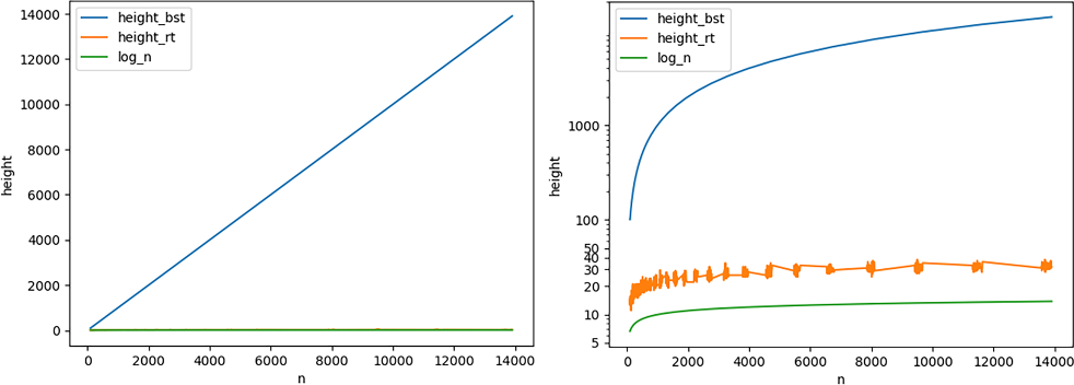
Figure 3.19 The height of a Randomized Treap versus a BST, after inserting the sequence 0, 1, . . . , n-1. The charts show the same data, on the left with linear scale and on the right using logarithmic scale for heights.
As expected, for BSTs the height is always not just linear in the number of nodes, but equal to the number of nodes (this time the slope is exactly 1), because the tree degenerates to a linked list, as expected.
Randomized Treaps, instead, keep performing well with logarithmic height, just like for the other tests, even in the most unfavorable case.
We can then conclude that if the parameter to improve is the height of the tree, Randomized Treaps do have an advantage in comparison to BSTs, and it is true that they keep a logarithmic height in all situations; therefore, their performance is comparable to more complex data structures such as red-black trees.
3.5.3 Profiling running time
The height of the tree, however, is not the only criteria we are interested in. We want to know if there is a catch, and what’s the price we have to pay in terms of running time and memory usage (figure 3.20).

Figure 3.20 Profiling CPU usage when inserting/removing random unbounded integers in a BST and Randomized Treap
To find out this, we run a proper profiling of the first test (with unbounded integers as keys, so with low or no duplicates) using JProfiler and recording the CPU time. The profiling used the implementations of BSTs and Randomized Treaps provided in the book’s repo. It’s worth noting that this profiling only gives us information on the implementations we examine, but we could get different results on optimized or differently designed software.
The results for our profiling run are shown in figure 3.20, where we can see that for insertion (method add) the cumulative running time spent for Randomized-Treap is almost twice as much as for BST::add; for method remove; instead, the ratio becomes 3.5 times.
From this first test, it seems that we pay a high price, in the general case, for the overhead due to the greater complexity of Randomized Treaps. This result is somehow expected, because when the height of the trees is approximately the same, the code for treaps is substantially more complex than for BSTs.
Should we just throw away our RandomizedTreap class? Well, not so fast. Let’s see what happens when we profile the second test case introduced in section 3.5.2, the one where we still add random integers to the containers, but limited to the range [0, 1000].
In the previous section, we saw that, in this case, BST’s height grows linearly, while for Randomized Treaps we still have a logarithmic growth.
Figure 3.21 shows the result of this profiling. We can immediately see that the situation has radically changed, and BSTs perform tremendously worse now. So much worse that BST::add takes 8-fold the running time of RandomizedTreap::add. For the method remove the ratio is even worse; we are talking about almost a 15-fold speed-up using Randomized Treaps—that’s exactly the situation where we would want to use our new, fancy, balanced data structure!

Figure 3.21 Profiling CPU usage when inserting/removing random integers between 0 and 1000 in a BST and Randomized Treap
For the sake of completeness, let’s also take a look at the worst-case scenario for BSTs. Figure 3.22 shows the profiling of the last test case introduced in section 3.5.2, where we insert an ordered sequence in our containers. In this case, I believe that the results don’t even need to be commented, because we are talking about thousands of seconds versus microseconds (we had to test on a smaller set because BSTs performance was so degraded as to be unbearably slow).
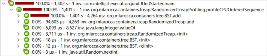
Figure 3.22 Profiling CPU usage when adding ordered sequences to a BST and Randomized Treap
All things considered, these results would suggest that if we are not sure about how uniform and duplicates-free the data we have to hold are, we should consider using Randomized Treaps. Instead, if we are sure the data will have lots of duplicates or possibly be close to sorted, then we definitely want to avoid using plain BSTs and resort to a balanced tree.
3.5.4 Profiling memory usage
So much for CPU usage, you might say, but what about memory usage? Because maybe Randomized Treaps are faster in some situations, but they require so much space that you won’t be able to store them in memory for large datasets.
First, we make a consideration: memory usage will be approximately the same for all the test cases we have introduced in the previous sections (when comparing containers of the same size, of course). This is because the number of nodes in both trees won’t change with their height; these trees do not support compression, and balanced and skewed trees will always need n nodes to store n keys.
Once we have established that, we can therefore be happy by profiling memory allocation for the most generic case, where the two trees are both approximately balanced. Figure 3.23 shows the cumulative memory allocated for the whole test for instances of the two classes.

Figure 3.23 Cumulative memory allocation for BST and RandomizedTreap, in the most generic case, with random insertions and removals
We can see that RandomizedTreap requires slightly more than twice the memory of BST. This is obviously not ideal, but is to be expected, considering that each node of a treap will hold a key (an Integer, in this test), plus a Double for the priority.
If we try a different kind of data for the keys—for instance, String—we can see that the difference becomes much smaller, as shown in figure 3.24. It’s just a ratio of 1.25 when storing strings between four and ten characters as keys.

Figure 3.24 Cumulative memory allocation for BST and RandomizedTreap when storing strings between 4 and 10 characters.
3.5.5 Conclusions
The analysis of the comparative performance and height of BSTs and Randomized Treaps suggests that, while the latter requires slightly more memory and can be slower in the generic case, when we don’t have any guarantee on the uniform distribution of keys or on the order of the operations, using BSTs carries a far greater risk of becoming a bottleneck.
If you remember, when we introduced data structures in chapter 1 we made it clear: knowing the right data structure to use is more about avoiding the wrong choices than finding the perfect data structure. This is exactly the same case. We (as developers) need to be aware of the situations where we need to use a balanced tree to avoid attacks or just degraded performance.
It’s worth reiterating that the first part of the analysis, focusing on the height of the trees, has general value21 and is independent of the programming language used. The analysis of running time and memory usage, instead, only has value for this implementation, programming language, design choices, and so on. All these aspects can, in theory, be optimized for your application’s specific requirements.
My advice, as always, is to carefully analyze requirements, understand what’s critical in your software and where you need certain guarantees about time and memory, and then test and profile the critical sections. Avoid wasting time on non-critical sections; usually you’ll find that the Pareto principle holds for software, and you can get an 80% performance gain by optimizing 20% of your code. Although the exact ratio may vary, the overall principle that you can get a significant improvement by optimizing the most critical parts of your application will likely hold.
Try to get a balance between clean code, time used to develop it, and efficiency. “Premature optimization is the root of all evil,” as stated by Donald Knuth,22 because trying to optimize all of your code will likely distract your team from finding the critical issues, and produce less-clean, less-readable, and less-maintainable code.
Always make sure to try to write clean code first, and then optimize the bottlenecks and the critical sections, especially those on which you have a service-level agreement, with requirements about time/memory used.
To give you a concrete example, the Java implementation we provide on the book’s repo makes heavy use of the Optional class (to avoid using null, and provide a nicer interface and a better way to handle unsuccessful searches/operations), and consequently also a lot of lambda functions.
If we profile in more detail the memory usage, disabling the filter on the package (to speed-up profiling, you usually want to avoid recording standard libraries, etc.), the final result is quite surprising, as we can see in figure 3.25.

Figure 3.25 Memory allocation by class for our test, without any filtering on the package
You can see that most space is used by instances of Optional and lambdas (implicitly created in Optional::map, etc.).
A complementary example for performance could be supporting multi-threading. If your application does not involve (ever) sharing these containers among different threads, you can avoid making your implementation thread-safe and save the overhead needed to create and synchronize locks.
Summary
-
Binary search trees offer good performance on all the typical container’s methods, but only if they’re kept balanced. Depending on the order of insertion of its keys, however, a BST can become skewed.
-
The edge case is when an ordered sequence is added to a BST, that will then contain a single path of length
n, de facto degenerating in a linked list. -
Treaps are a hybrid between BSTs and heaps, abiding by BST’s invariants for keys, and heap’s invariants for priorities.
-
If we randomly assign priorities, drawing them from a uniform continuous set (such as, but not limited to, all real numbers between 0 and 1), we can mathematically guarantee that for large enough values of
n, the tree will storenelements and maintain a height not greater than2*log(n). -
Besides the theoretical guarantees, it’s possible to verify (as we did with Java implementations) that Randomized Treaps will keep a logarithmic height even in the worst-case scenarios for BSTs.
-
Moreover, the performance in term of CPU running time and memory usage is comparable for both data structures in the general case, and much better for Randomized Treaps in the edge cases where BSTs struggle.
1. Treaps were introduced in the paper “Randomized search trees,” by Cecilia R. Aragon and Raimund C. Seidel, 30th Annual Symposium on Foundations of Computer Science. IEEE, 1989. Although the title of the paper might be misleading, we will see later in this chapter how treaps are related to randomized search trees.
2. A portmanteau is a blend of two or more words, where parts of each word are combined into a new word.
3. As we discussed in chapter 2, “higher priority” is an abstraction that can mean lower or higher values, depending on the type of heap we are using. Here we are dealing with a min-heap, and higher priority means “lower inventory count,” so smaller values go to the top. The code also assumes we are implementing a min-heap.
4. Red-black and 2-3 trees are fancy versions of balanced BSTs. We’ll talk more about them in a few sections.
5. See https://github.com/mlarocca/AlgorithmsAndDataStructuresInAction#treap.
6. You can read more about the issue with stack overflow and tail call optimization in appendix E.
7. In our example, the lowest priority corresponds to the highest availability in stock, and so +∞ is the highest possible value for the units in stock.
8. Remember that in a heap, elements are partially ordered by priority, but not ordered at all by key. We can get the element with the highest priority, but to get the smallest (or largest) key, we need to check all elements.
9. Aho, Alfred V., and John E. Hopcroft. The design and analysis of computer algorithms. Pearson Education India, 1974.
10. Guibas, Leo J., and Robert Sedgewick. “A dichromatic framework for balanced trees.” 19th Annual Symposium on Foundations of Computer Science (sfcs 1978). IEEE, 1978.
11. Meant as balanced, with a high probability.
12. See https://github.com/mlarocca/AlgorithmsAndDataStructuresInAction#treap.
13. See appendix C for a recap on hashing.
14. It goes without saying that this holds if the pseudo-random generators are implemented properly and within the limits caused by the fact that a classic computer can’t offer true randomness. Either way, we make the attackers’ job a little harder.
15. Assuming i < k; otherwise, if i > k, we refer the subset {Nk, Nk+1, ... Ni-1, Ni}.
16. JProfiler is a commercial tool. You can find open-source alternatives that will also get the job done.
17. https://github.com/mlarocca/AlgorithmsAndDataStructuresInAction/blob/master/Java/tests/org/mlarocca/containers/treap/RandomizedTreapProfiling.java.
18. https://github.com/mlarocca/AlgorithmsAndDataStructuresInAction/blob/master/Java/src/org/mlarocca/ containers/tree/BST.java.
19. The standard implementation of the remove method in BSTs, when the node N to remove has both children, uses the node’s successor to replace the key to delete (and then recursively delete this successor). Over a long number of removals, this causes the tree to become skewed, left-leaning. A solution to mitigate this effect is randomly deciding, with a 50% probability, to use the predecessor of a key instead of its successor.
20. Stack overflow, its relation with recursion, and how to avoid such crashes is explained in appendix E.
21. Assuming the algorithms are implemented verbatim, it’s also not dependent on the specific implementation.
22. “The real problem is that programmers have spent far too much time worrying about efficiency in the wrong places and at the wrong times. Premature optimization is the root of all evil (or at least most of it) in programming.” Knuth, Donald Ervin. The art of computer programming. Pearson Education, 1997.